Final Analysis of Proton Form Factor Ratio Data at $\mathbf{Q^{2}=4.0}$, 4.8 and 5.6 GeV²

Abstract

Precise measurements of the proton electromagnetic form factor ratio $R=\mu_{p}G_{E}^{p}/G_{M}^{p}$ using the polarization transfer method at Jefferson Lab have revolutionized the understanding of nucleon structure by revealing the strong decrease of $R$ with momentum transfer $Q^{2}$ for $Q^{2}\gtrsim 1$ GeV², in strong disagreement with previous extractions of $R$ from cross section measurements. In particular, the polarization transfer results have exposed the limits of applicability of the one-photon-exchange approximation and highlighted the role of quark orbital angular momentum in the nucleon structure. The GEp-II experiment in Jefferson Lab’s Hall A measured $R$ at four $Q^{2}$ values in the range $3.5$ GeV${}^{2}\leq Q^{2}\leq 5.6$ GeV². A possible discrepancy between the originally published GEp-II results and more recent measurements at higher $Q^{2}$ motivated a new analysis of the GEp-II data. This article presents the final results of the GEp-II experiment, including details of the new analysis, an expanded description of the apparatus and an overview of theoretical progress since the original publication. The key result of the final analysis is a systematic increase in the results for $R$, improving the consistency of the polarization transfer data in the high-$Q^{2}$ region. This increase is the result of an improved selection of elastic events which largely removes the systematic effect of the inelastic contamination, underestimated by the original analysis.

I Introduction

The electromagnetic form factors (FFs) of the nucleon have been revived as a subject of high interest in hadronic physics since a series of precise recoil polarization measurements of the ratio of the proton’s electric ($G_{E}^{p}$) and magnetic ($G_{M}^{p}$) FFs Jones et al. (2000); *Punjabi05; *Punjabi05erratum; Gayou et al. (2002) in Jefferson Lab’s Hall A established the rapid decrease with momentum transfer $Q^{2}$ of $R=\mu_{p}G_{E}^{p}/G_{M}^{p}$, where $\mu_{p}$ is the proton’s magnetic moment, for 0.5 GeV${}^{2}\leq Q^{2}\leq 5.6$ GeV². These measurements disagreed strongly with previous extractions of $G_{E}^{p}$ from cross section data Perdrisat et al. (2007) using the Rosenbluth method Rosenbluth (1950), which found $\mu_{p}G_{E}^{p}/G_{M}^{p}\approx 1$. Subsequent investigations of both experimental techniques, including a novel “Super-Rosenbluth” measurement using ${}^{1}H(e,p)e^{\prime}$ cross section measurements to reduce systematic uncertainties Qattan et al. (2005), found no neglected sources of error in either data set, pointing to incompletely understood physics as the source of the discrepancy.

Theoretical investigations of the discrepancy have focused on higher-order QED corrections to the cross section and polarization observables in elastic $ep$ scattering Afanasev et al. (2001); Carlson and Vanderhaeghen (2007), including radiative corrections and two-photon-exchange (TPEX) effects. The amplitude for elastic electron-proton scattering involving the exchange of two or more hard photons cannot presently be calculated model-independently. In the $Q^{2}$ region of the discrepancy, model calculations of TPEX Blunden et al. (2005); Afanasev et al. (2005) predict relative corrections to both the cross section and polarization observables that are typically at the few-percent level. At large $Q^{2}$, the sensitivity of the Born (one-photon-exchange) cross section to $G_{E}^{p}$ becomes similar to or smaller than the sensitivity of the measured cross section to poorly-known TPEX corrections, obscuring the extraction of $G_{E}^{p}$. On the other hand, the polarization transfer ratio $R$ defined in equations (I) is directly proportional to $G_{E}^{p}/G_{M}^{p}$, such that the extraction of $G_{E}^{p}$ is much less sensitive to corrections beyond the Born approximation. For this reason, a general consensus has emerged that the polarization transfer data most reliably determine $G_{E}^{p}$ at large $Q^{2}$. Nonetheless, active experimental and theoretical investigation of the discrepancy and the role of TPEX continues Arrington et al. (2011). Owing to the lack of a model-independent theoretical prescription for TPEX corrections, precise measurements of elastic $ep$ scattering observables sensitive to TPEX effects continue to play an important role in the resolution of the discrepancy.

The revised experimental understanding of the proton form factors led to an onslaught of theoretical work. The constancy of the Rosenbluth data for $G_{E}^{p}/G_{M}^{p}$ was consistent with a “precocious” onset of pQCD dimensional scaling laws Brodsky and Farrar (1975); *BrodskyLepage1979, valid for asymptotically large $Q^{2}$, an interpretation which had to be abandoned in light of the polarization data. The decrease of $R$ with $Q^{2}$ was later interpreted in a pQCD-scaling framework including higher-twist corrections Belitsky et al. (2003), demonstrating the importance of quark orbital angular momentum in the interpretation of nucleon structure. The relations between nucleon form factors and Generalized Parton Distributions (GPDs) have placed this connection on a more quantitative footing Ji (1997a); Guidal et al. (2005); Diehl et al. (2005). Furthermore, the GPD-form factor sum rules have been used to derive model-independent representations of the nucleon transverse charge and magnetization densities as two-dimensional Fourier transforms of the Dirac ($F_{1}$) and Pauli ($F_{2}$) form factors Miller (2007); *MillerGPDmagnetdensity2008. In the context of calculations based on QCD’s Dyson-Schwinger Equations (DSEs) Cloët et al. (2009); Eichmann (2011), the form factor data are instrumental in elucidating the dynamical interplay between the nucleon’s dressed-quark core, diquark correlations, and the pseudoscalar meson cloud Roberts (2008). Recent measurements of the neutron form factors at large $Q^{2}$ Riordan et al. (2010); Lachniet et al. (2009) have enabled for the first time a detailed flavor-decomposition Cates et al. (2011) of the form factor data, leading to new insights. In addition, the form factor data have been interpreted within a large number of phenomenological models; a recent review of the large body of theoretical work relevant to the nucleon FFs is given in Perdrisat et al. (2007), and a current overview is given in section IV.2 of this work.

The recoil polarization method exploits the relation between the transferred polarization in elastic $\vec{e}p$ scattering and the ratio $G_{E}^{p}/G_{M}^{p}$. In the one-photon-exchange approximation, the polarization transferred to recoiling protons in the elastic scattering of longitudinally polarized electrons by unpolarized protons has longitudinal ($P_{\ell}$) and transverse ($P_{t}$) components in the reaction plane given by Akhiezer and Rekalo (1968a); *AkhiezerRekalo1; *AkhiezerRekalo2; Arnold et al. (1981)

$$P_{t} = -hP_{e}\sqrt{\frac{2\epsilon(1-\epsilon)}{\tau}}\frac{r}{1+\frac{\epsilon}{\tau}r^{2}}$$

$$P_{\ell} = hP_{e}\frac{\sqrt{1-\epsilon^{2}}}{1+\frac{\epsilon}{\tau}r^{2}}$$ (1)

$$r\equiv\frac{G_{E}^{p}}{G_{M}^{p}} = -\frac{P_{t}}{P_{\ell}}\sqrt{\frac{\tau(1+\epsilon)}{2\epsilon}}=\frac{R}{\mu_{p}},$$

where $h=\pm 1$ is the electron beam helicity, $P_{e}$ is the beam polarization, $\tau\equiv Q^{2}/4M_{p}^{2}$, $M_{p}$ is the proton mass, and $\epsilon\equiv\left[1+2(1+\tau)\tan^{2}\left(\theta_{e}/2\right)\right]^{-1}$, with $\theta_{e}$ the electron scattering angle in the proton rest (lab) frame, corresponds to the longitudinal polarization of the virtual photon in the one-photon-exchange approximation.

Recent measurements from Jefferson Lab’s Hall C Puckett et al. (2010) extended the $Q^{2}$ reach of the polarization transfer method to 8.5 GeV². The published data from Hall A are well described by a linear $Q^{2}$ dependence Perdrisat et al. (2007),

$$R=1.0587-0.14265Q^{2},$$ (2)

with $Q^{2}$ in GeV², valid for $Q^{2}\geq 0.4$ GeV². On the other hand, all three of the recent Hall C data points are at least 1.5 standard deviations above this line, including the measurement at overlapping $Q^{2}=5.17$ GeV², which lies 1.8$\sigma$ above equation (2). Due to the strong, incompletely understood discrepancy between the Rosenbluth and polarization transfer methods of extracting $G_{E}^{p}/G_{M}^{p}$ and the fact that the new Hall C measurements are the first to check the reproducibility of the Hall A data using a completely different apparatus in the $Q^{2}$ region where the discrepancy is strongest, understanding possible systematic differences between the experiments is important.

This article reports an updated, final data analysis of the three higher-$Q^{2}$ measurements of $R$ from Hall A, originally published in Gayou et al. (2002), along with expanded details of the experiment. To avoid confusion, a naming convention is adopted throughout the remainder of this article for the most frequently cited experiments: GEp-I for Ref. Punjabi et al. (2005a), GEp-II for Ref. Gayou et al. (2002), the subject of this article, GEp-III for Ref. Puckett et al. (2010) and GEp-2$\gamma$ for Ref. Meziane et al. (2011). Section II presents the kinematics of the measurements, an expanded description of the experimental apparatus, and a comparison of the GEp-II and GEp-III/GEp-2$\gamma$ experiments. Section III presents the data analysis method, including the selection of elastic events, the extraction of polarization observables, and the estimation and subtraction of the non-elastic background contribution. Section IV presents the final results of the experiment and discusses the impact of the revised data on the world database of proton electromagnetic form factor measurements, in the context of the considerable advances in theory since the original publication. The conclusions and summary are given in section V.

II Experiment Setup

Table 1 shows the central kinematics of the measurements from the GEp-II experiment. The kinematic variables given in Table 1 are the beam energy $E_{e}$, the scattered electron energy $E^{\prime}_{e}$, the electron scattering angle $\theta_{e}$, the scattered proton momentum $p_{p}$, and the proton scattering angle $\theta_{p}$.

Table 1: Central kinematics of the GEp-II experiment. The central $Q^{2}$ value is defined by the central momentum of the left HRS in which the proton was detected. $\epsilon$ is the parameter appearing in equation (I), $E_{e}$ is the beam energy, $E^{\prime}_{e}$ is the scattered electron energy, $\theta_{e}$ is the electron scattering angle, $p_{p}$ is the proton momentum, $\theta_{p}$ is the proton scattering angle, $\chi$ is the central spin precession angle, $P_{e}$ is the beam polarization, and $R_{cal}$ is the distance from the target to the calorimeter surface. At the lowest $Q^{2}$ of 3.5 GeV², the scattered electron was detected in the right HRS.

Nominal $Q^{2}$ (GeV2)	$\epsilon$	$E_{e}$ (GeV)	$E^{\prime}_{e}$ (GeV)	$\theta_{e}$ (∘)	$p_{p}$ (GeV)	$\theta_{p}$ (∘)	$\chi$ (∘)	$P_{e}$ (%)	$R_{cal}$ (m)
3.5	0.77	4.61	2.74	30.6	2.64	31.8	241	70	HRSR
4.0	0.71	4.61	2.47	34.5	2.92	28.6	264	70	17.0
4.8	0.59	4.59	2.04	42.1	3.36	23.8	301	73	12.5
5.6	0.45	4.60	1.61	51.4	3.81	19.3	337	71	9.0

II.1 Experimental Apparatus

The GEp-II experiment ran in Hall A at Jefferson Lab during November and December of 2000. A polarized electron beam was scattered off a liquid hydrogen target. Hall A is equipped with two High Resolution Spectrometers (HRS) Alcorn et al. (2004), which are identical in design. In this experiment, the left HRS (HRSL) was used to detect the recoil proton, while the right HRS (HRSR) was used to detect the scattered electron at the lowest $Q^{2}$ of 3.5 GeV². For the three highest $Q^{2}$ points at 4.0, 4.8 and 5.6 GeV², electrons were detected by a lead-glass calorimeter. The focal plane of the HRSL was equipped with a focal plane polarimeter (FPP) to measure the polarization of the recoil proton.

The Continuous Electron Beam Accelerator at the Thomas Jefferson National Accelerator Facility (JLab) delivers a high quality, longitudinally polarized electron beam with $\sim$100% duty factor. The beam energy was measured using the Arc and ep methods. The ep method determines the energy by measuring the opening angle between the scattered electron and the recoil proton in ep elastic scattering, while the Arc method uses the standard technique of measuring a bend angle in a series of dipole magnets. The combined absolute accuracy of both methods is $\Delta E/E\sim 10^{-4}$, while the beam energy spread is at the $10^{-5}$ level. The nominal beam energy in this experiment was 4.6 GeV. The beam polarization was measured by Compton and Möller polarimeters. Details of the standard Hall A equipment can be found in Alcorn et al. (2004) and references therein.

The hydrogen target cell used in this experiment was 15 cm long along the beam direction. The target was operated at a constant temperature of 19 K and pressure of 25 psi, resulting in a density of about 0.072 g/cm³. To minimize the target density fluctuations due to localized heat deposition by the intense electron beam, a fast raster system consisting of a pair of dipole magnets was used to increase the transverse size of the beam in the horizontal and vertical directions. The raster shape was square or circular in the plane transverse to the beam axis. In this experiment, the raster size was approximately $4\times 4$ mm².

Recoil protons were detected in the high resolution spectrometer located on the beam left (HRSL) Alcorn et al. (2004). The HRSL has a central bend angle of $45^{\circ}$, and subtends a $6.5$ msr solid-angle for charged particles with momenta up to 4 GeV with $\pm 5\%$ momentum acceptance. Two vertical drift chambers measure the particle’s position and trajectory at the focal plane. With knowledge of the optics of the HRSL magnets and precise beam position monitoring, the proton scattering angles, momentum and vertex coordinates were reconstructed with FWHM resolutions of $\sim$2.6 (4.0) mrad for the in-plane (out-of-plane) angle, $\Delta p/p\sim 2.6\times 10^{-4}$ for the momentum, and $\sim$3.1 mm for the vertex coordinate in the plane transverse to the HRSL optical axis.

II.1.1 Focal Plane Polarimeter

The central instrument of this experiment was the Focal Plane Polarimeter (FPP) Punjabi et al. (2005a), installed in the focal plane of HRSL. The FPP measures the transverse polarization of the recoil proton. The protons are scattered in the focal plane region by an analyzer, as shown in Figure 1. If the protons are polarized transverse to their momentum direction, an azimuthal asymmetry results from the spin-orbit interaction with the analyzing nuclei.

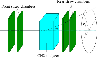
Figure 1: (color online) Layout of the Focal Plane Polarimeter.

The FPP has been described in detail in Punjabi et al. (2005a), so only a brief summary of its characteristics will be given here. The only significant difference in the configuration of the FPP between the GEp-I and GEp-II experiments was a change of the analyzer material from carbon to polyethylene. During GEp-I, the analyzer consisted of four doors of carbon which could be combined to produce a maximum thickness of 51 cm. For cost, safety and efficiency reasons, carbon is ideal for measuring proton polarization with a momentum up to 2.4 GeV, which was sufficient for GEp-I. For GEp-II, the maximum proton momentum was 3.8 GeV. At this momentum, the analyzing power of carbon, which contributes to the size of the asymmetry, and therefore to the size of the error bar, decreases significantly. An experiment was carried out at the Laboratory for High Energy (LHE) at the Joint Institute for Nuclear Research (JINR) in Dubna, Russia to find an optimal analyzing material and its thickness for protons at 3.8 GeV Azhgirey et al. (2005). Polyethylene, a compound of carbon and hydrogen, was found to increase the analyzing power relative to carbon as shown in Figure 2. A stack of eighty 2.5 cm-thick plates, each 58 cm deep along the direction of incident protons, was installed between the unused, opened, doors of the carbon analyzer, as shown in Figure 3. This 58 cm thickness was used for the $Q^{2}$ = 3.5 GeV² kinematics. For the three higher $Q^{2}$ kinematics, an additional stack of polyethylene with a thickness of 42 cm was installed on a rail just upstream of the 58 cm stack to give a total thickness of 100 cm.

Figure 2: (color online) Analyzing power versus scattering angle in the analyzer for graphite (49.5 cm-thick) and polyethylene (58 cm-thick) at a proton momentum of 2.64 GeV, corresponding to $Q^{2}=3.5$ GeV².

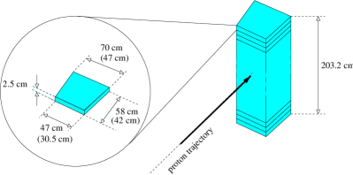
Figure 3: (color online) Stack of polyethylene plates for the analyzer. The dimensions shown on the plate are for the 58 cm (42 cm) stack, and were chosen to match the envelope of elastically scattered protons in HRSL.

II.1.2 Electron detection at $Q^{2}=3.5$ GeV²

For the measurement at $Q^{2}=3.5$ GeV², the electron was detected in the high resolution spectrometer located on the beam right (HRSR). The trigger was defined by a coincidence between an electron in HRSR and a proton in HRSL. The precise measurement of the scattered electron kinematics using a high-resolution magnetic spectrometer provides for an extremely clean selection of elastic $ep$ events with cuts on the reconstructed missing energy and momentum, as shown in Fig. 4.8 of Ref. Gayou (2002).

II.1.3 Electron detection at $Q^{2}\geq 4.0$ GeV²

For the measurements at $Q^{2}\geq 4.0$ GeV², a lead-glass calorimeter was used to detect electrons due to the larger electron solid angle compared to the proton solid angle defined by HRSL. The lead-glass blocks from the standard HRSR calorimeter were used to assemble this calorimeter along with some additional spare blocks. Figure 4 shows a front and a side view of the calorimeter on its platform. The blocks of lead-glass, of cross-sectional area $15\times 15$ cm², were individually wrapped in one foil of aluminized mylar, and one foil of black paper, to avoid light leaks. Each block was then tested, and the current drawn in the phototube due to noise was found to be less than 100 nA for all blocks. The blocks were assembled in a rectangular array of 9 columns and 17 rows, requiring a total of 153 blocks. Most of the blocks, in green in Figure 4, were 35 cm long, corresponding to 13.7 radiation lengths. 37 blocks positioned on the edges of the calorimeter were only 30 cm long, corresponding to 11.8 radiation lengths (in blue in Figure 4). The highest electron energy, at $Q^{2}$ = 4.0 GeV², was 2.5 GeV. At this energy, the shower stops after 7.7 radiation lengths, so that the entire shower is contained in the block. Since only 147 blocks were available, 6 blocks were missing to form a complete rectangle. These were replaced by wood placeholder blocks at the corners of the detector (in red in Figure 4). The active area of the calorimeter was 3.31 m².

The blocks were placed in the steel support frame (1), and held together using wood plates (2). The front of the support was covered with a one inch thick aluminum plate (3) to absorb very low energy particles. The ensemble was lifted by the top steel plate (4) onto the platform (5) using the Hall A crane. Balance on the platform was maintained by the steel support legs (6). The ensemble was placed on wheels and moved with the help of the Hall A crane attached to the steel lifting frame (7). The calorimeter was placed at the distance from the target required to match the electron solid angle to that of the proton at each kinematic setting. The acceptance matching was only approximate, due to the complicated shape of the spectrometer acceptance. Overall, about 5% of elastic events with a proton detected in HRSL were lost due to acceptance mismatching. The Cherenkov light emitted by primary electrons and shower secondaries in the lead-glass was collected by Photonis XP2050 photomultipliers (8), and the signals were digitized by LeCroy 1881 integrating ADCs and LeCroy 1877 TDCs.

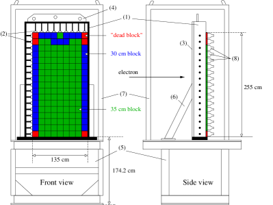
Figure 4: (color) Design of the calorimeter used to detect the scattered electron. In the front view, the 2.54 cm-thick aluminum plate in front of the blocks is not shown. See text for details.

The trigger for the measurements at $Q^{2}\geq 4.0$ GeV² was defined by a single proton in the HRS, signaled by a coincidence of two planes of scintillators in the focal plane. For each single proton event in the left HRS, the ADC and TDC information from the calorimeter was read out for all blocks, and elastic events were selected offline by applying software cuts to the calorimeter data.

II.2 Comparison to Hall C Experiments

The GEp-II experiment shares several important features with GEp-III. Both experiments used magnetic spectrometers instrumented with Focal Plane Polarimeters (FPPs) to detect protons and measure their polarization, and large acceptance electromagnetic calorimeters to detect electrons in coincidence. The use of calorimeters in both experiments was driven by the requirement of acceptance matching; at large $Q^{2}$ and $\theta_{e}$, the Jacobian of the reaction magnifies the electron solid angle compared to the proton solid angle fixed by the spectrometer acceptance. The drawbacks of this choice compared to electron detection using a magnetic spectrometer are twofold. First, the energy resolution of lead-glass calorimeters is relatively poor, so that elastic and inelastic reactions are not well separated in reconstructed electron energy. Second, the signals in lead-glass from electrons and photons of similar energies are indistinguishable, leaving one vulnerable to photon backgrounds from the decay of $\pi^{0}$, which played an important role in the analysis of both experiments.

The high-$Q^{2}$ measurements of the GEp-III experiment Puckett et al. (2010) were carried out consecutively with the GEp-2$\gamma$ experiment, a series of precise measurements of $R$ at $Q^{2}=2.5$ GeV² Meziane et al. (2011) designed to search for effects beyond the Born approximation, thought to explain the disagreement between Rosenbluth and polarization data Carlson and Vanderhaeghen (2007). Using the same apparatus and analysis procedure as GEp-III, the results of GEp-$2\gamma$ Meziane et al. (2011) are in excellent agreement with the GEp-I data from Hall A Punjabi et al. (2005a) at nearly identical $Q^{2}$, as shown in Figure 12. The background corrections to the GEp-2$\gamma$ data were negligible after applying the cuts described in Puckett et al. (2010); Meziane et al. (2011). Similarly, electrons were detected in the HRSL in the GEp-I experiment, so that the selection of elastic events was practically background-free Punjabi et al. (2005a). In the absence of major background corrections, the agreement between precise measurements at the same $Q^{2}$ using different polarimeters and magnetic spectrometers limits the size of any potentially neglected systematic errors arising from sources other than background.

The liquid hydrogen targets used in Halls A and C had radiation lengths of $\sim$2%, leading to a significant Bremsstrahlung flux across the target length, in addition to the virtual photon flux due to the presence of the electron beam. The kinematics of $\pi^{0}$ photoproduction ($\gamma+p\rightarrow\pi^{0}+p$) near end point ($E_{\gamma}\rightarrow E_{e}$) are very similar to elastic $ep$ scattering at high energies ($E_{\gamma}\gg m_{\pi}$), such that protons from $\gamma+p\rightarrow\pi^{0}+p$ overlap with elastically scattered protons within experimental resolution. In the lab frame, asymmetric $\pi^{0}$ decays with one photon emitted at a forward angle relative to the $\pi^{0}$ momentum, carrying most of the $\pi^{0}$ energy, are detected with a high probability. At high energies and momentum transfers, the $\pi^{0}$ photoproduction cross section is observed to scale as $s^{-7}$ for fixed $\Theta_{CM}$ Anderson et al. (1976), where $s$ is the center-of-momentum (CM) energy squared and $\Theta_{CM}$ is the CM $\pi^{0}$ production angle. In addition, the CM angular distribution is peaked at forward and backward angles. The goal of the GEp-III experiment was to measure to the highest possible $Q^{2}$, given the maximum available beam energy of 5.71 GeV. At $Q^{2}=8.5$ GeV², the relatively high $Q^{2}/s$ ratio, with $\Theta_{CM}\in$ 129-143^∘, led to a $\pi^{0}p$:$ep$ ratio of $\sim$40:1. The severity of the background conditions required maximal exploitation of elastic kinematics to suppress the $\pi^{0}$ background. Even after all cuts described in Puckett et al. (2010), the remaining background was estimated at $\sim$6% of accepted events. Given the large difference between the signal and background polarizations, this level of contamination required a substantial positive correction to $R$.

In light of the improved understanding of the importance of the $\pi^{0}$ background gained during the analysis of the GEp-III data, an underestimation of its effect in the GEp-II analysis was considered as a potential source of disagreement between the two experiments. Therefore, the GEp-II data for $Q^{2}=$ 4.0, 4.8, and 5.6 GeV² were reanalyzed to investigate the systematics of the $\pi^{0}$ background. The data from GEp-II at $Q^{2}=3.5$ GeV² were not reanalyzed, since electrons were detected in the HRSR and the $\pi^{0}$ background was absent. The systematics of this configuration were thus irrelevant to the comparison between GEp-II and GEp-III at higher $Q^{2}$.

III Data Analysis

III.1 Elastic Event Selection

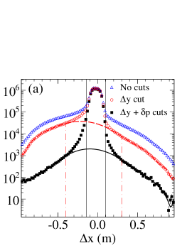
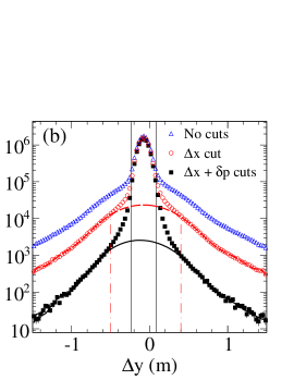
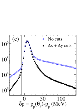
Figure 5: (color online) Elastic event selection at $Q^{2}=4.8$ GeV². The effects of cuts are shown for the horizontal calorimeter coordinate difference $\Delta x$ in panel (a), the vertical difference $\Delta y$ in panel (b), and the proton momentum difference $\delta p\equiv p_{p}(\theta_{p})-p_{p}$ in panel (c). Solid vertical lines indicate the cut applied. Empty triangles show the distribution of events before applying any cuts. Filled squares show events passing the cuts on both of the other two variables. Empty circles in panels (a) and (b) show the $\Delta x$ ($\Delta y$) distribution of events passing the $\Delta y$ ($\Delta x$) cut, regardless of $\delta p$. In panels (a) and (b), the dashed and solid curves show the estimated background before and after the $\delta p$ cut. Dot-dashed vertical lines indicate the range of the elastic peak excluded from the fit to the background.

Figure 5 shows a representative example of the procedure for isolating elastic events in the GEp-II data, at $Q^{2}=4.8$ GeV². As described in Gayou et al. (2002) and Gayou (2002), cuts were applied to the difference between the HRS and calorimeter time signals ($\pm 4$ ns at $Q^{2}=4.0$ and 4.8 GeV², and $\pm 5$ ns at $Q^{2}=5.6$ GeV²) and the missing energy $\left(\left|E_{miss}\equiv E_{e}+M_{p}-\sqrt{p_{p}^{2}+M_{p}^{2}}-E_{calo}\right|\leq 1000\mbox{ MeV}\right)$ to suppress random coincidences and low-energy inelastic backgrounds, respectively. The remaining backgrounds from ¹H$(\gamma,\pi^{0}p)$ and quasielastic Al$(e,e^{\prime}p)$ reactions in the target cell windows were rejected using the kinematic correlations between the electron and proton arms. The measured proton kinematics were used to predict the scattered electron’s trajectory assuming elastic scattering, and then the predicted electron trajectory, defined by the polar scattering angle $\theta_{e}^{(p)}$ and the azimuthal scattering angle $\phi_{e}^{(p)}$ (where ^(p) denotes the value predicted from the measured proton kinematics), was projected from the measured interaction vertex to the surface of the calorimeter.

Figures 5(a) and 5(b) show the horizontal ($\Delta x$) and vertical ($\Delta y$) differences between the measured shower coordinates at the calorimeter and the coordinates calculated from the measured proton kinematics assuming elastic scattering. Figure 5(c) shows the difference $\delta p\equiv p_{p}(\theta_{p})-p_{p}$ between the measured $p_{p}$ and the momentum required by elastic kinematics at the measured $\theta_{p}$, given by

$$p_{p}(\theta_{p}) = \frac{2M_{p}E_{e}(M_{p}+E_{e})\cos\theta_{p}}{M_{p}^{2}+2M_{p}E_{e}+E_{e}^{2}\sin^{2}\theta_{p}}.$$ (3)

In each panel of Figure 5, the distribution of the plotted variable is shown before and after applying cuts (illustrated by vertical lines) to both of the other two variables, which most nearly corresponds to the GEp-III analysis. In addition, the $\Delta x$ ($\Delta y$) distribution is shown after applying the cut to $\Delta y$ ($\Delta x$), regardless of $\delta p$, which most nearly corresponds to the selection of the original GEp-II analysis, in which no cut was applied to $\delta p$. Each spectrum exhibits a clear elastic peak near zero on top of a smooth background distribution. The background in the $\Delta x$ and $\Delta y$ spectra is dominated by $\pi^{0}$ photoproduction events. The estimated background curves shown in panels (a) and (b) of Figure 5 were obtained using the polynomial sideband fitting method described in section III.3.2. The $\delta p$ cut clearly has significant additional background suppression power relative to $\Delta x$ and $\Delta y$ cuts alone. In the $\delta p$ spectrum, the background distribution is highly asymmetric about the peak, reflecting the fact that elastically scattered protons carry the highest kinematically allowed momenta at a given $\theta_{p}$.

Since the two-body reaction kinematics are overdetermined, the method used to calculate $\Delta x$ and $\Delta y$ is not unique. In combination with the precisely known beam energy, the expected electron polar scattering angle $\theta_{e}^{(p)}$ can be calculated from either the measured proton momentum $p_{p}$, the measured proton scattering angle $\theta_{p}$, or a combination of both. Different methods were used by the GEp-II and GEp-III data analyses to calculate $\Delta x$ and $\Delta y$. In the original GEp-II analysis, the calculation was formulated in terms of Cartesian components of the outgoing particle momenta rather than polar and azimuthal scattering angles. The effective $\theta_{e}^{(p)}$ in the GEp-II approach depends on both $\theta_{p}$ and $p_{p}$. The exact equations used can be found in Appendix D of Ref. Gayou (2002). In the GEp-III analysis, $\theta_{e}^{(p)}$ was calculated from $p_{p}$, as described in Puckett et al. (2010). Both methods were tested in the present reanalysis. The $\Delta x$ and $\Delta y$ distributions in Figures 5(a) and 5(b) were calculated using the GEp-II method, in order to demonstrate the background suppression power of the added $\delta p$ cut of Fig. 5(c) relative to the original analysis. For events selected by this cut, $p_{p}\approx p_{p}(\theta_{p})$, such that the $\Delta x$ values obtained from the GEp-II and GEp-III methods are equal up to detector resolution.

A key difference between the GEp-III and GEp-II experiments is the dominant source of resolution in the variables used to select elastic events. The cell size of the GEp-II calorimeter was 15 $\times$ 15 cm², compared to the 4 $\times$ 4 cm² cell size of the GEp-III calorimeter. In GEp-II, the resolution of $\Delta x$ and $\Delta y$ is dominated by the calorimeter coordinate measurement, and is therefore largely insensitive to the choice of proton variables used to calculate the expected electron angles. In GEp-III, on the other hand, the scattered electron angles were measured with excellent resolution by the highly-segmented BigCal, such that the proton arm resolution was dominant. Given the kinematics of GEp-III and the angular and momentum resolution of the High Momentum Spectrometer (HMS) in Hall C Blok et al. (2008), the best $\Delta x$ resolution was obtained by using $p_{p}$ to calculate $\theta_{e}^{(p)}$. In the GEp-II analysis, the main practical difference between the two methods is the resulting background shape. In kinematics for which the reaction Jacobian necessitates the use of a calorimeter for electron detection, the GEp-III method generally results in a wider and more asymmetric $\Delta x$ distribution of the background, with inelastic events assuming predominantly negative $\Delta x$ values. In the GEp-III analysis, using $\theta_{e}^{(p)}(p_{p})$ provided the best possible $\Delta x$ resolution and a wider $\Delta x$ distribution of the background. In the GEp-II case, calculating $\Delta x$ using the GEp-III method spreads out the background without affecting the width of the elastic peak, thus reducing the background in the $\Delta x$ spectrum with no $\delta p$ cut. After applying the $\delta p$ cut, however, the $\Delta x$ distributions obtained from the two calculations are practically identical, and the choice becomes arbitrary. As discussed in section III.4, the results for $R$ obtained with the $\delta p$ cut included do not depend on the method used to calculate $\Delta x$. The final reanalysis results were obtained with $\Delta x$ and $\Delta y$ calculated using the GEp-II method.

The original GEp-II analysis applied a two-dimensional polygon cut to the correlated $\Delta y$ versus $\Delta x$ distribution. Using identical cuts to the original analysis, the published results Gayou et al. (2002) were successfully reproduced. In the final analysis, however, one-dimensional (rectangular) cuts were applied to $\Delta x$ and $\Delta y$, which simplifies the background estimation procedure. For all three $Q^{2}$ points, a cut of $\pm 12(\pm 16)$ cm was applied to $\Delta x$($\Delta y$), centered at the midpoint between half-maxima on either side of the elastic peak, as in Figure 5. The width of the cuts was chosen to be similar to the effective width of the polygon cut applied by the original analysis, and reflects the dominant contribution of the calorimeter cell size to the resolution of $\Delta x$ and $\Delta y$. In addition, a cut of $\pm 15$ MeV, also centered at the midpoint between half-maxima of the elastic peak, was applied to $\delta p$, as in Figure 5(c). The width of the $\delta p$ cut was chosen to be $\pm 3\sigma$, where $\sigma\approx 5$ MeV is the $\delta p$ resolution, which was roughly independent of the proton momentum in this experiment. While the difference in the selection of events from using a different shape of the $\Delta x$ and $\Delta y$ cuts is small, the $\delta p$ cut removes a rather substantial 6.0%, 7.3%, and 10.7% of events relative to the original analysis for $Q^{2}=4.0$, 4.8 and 5.6 GeV², respectively.

While a fraction of the events rejected by the $\delta p$ cut are elastic, including events in the $ep$ radiative tail and elastic events with $\delta p$ smeared by non-Gaussian tails of the HRS resolution, most of the rejected events are part of the background, and contribute very little to the statistical precision of the data. Moreover, even real elastic events reconstructed outside the peak region of $\delta p$ do not meaningfully contribute to the accurate determination of the form factor ratio, because such events are either (a) part of the radiative tail and therefore subject to radiative corrections that are in principle calculable Afanasev et al. (2001) but practically difficult due to large backgrounds in the radiative tail region, or (b) have unreliable angle or momentum reconstruction, which distorts the spin transport matrix of the HRS (see Ref. Ron et al. (2011) and section III.2.2 below) in an uncontrolled fashion. Therefore, the application of the $\delta p$ cut has benefits beyond mere background suppression, as it also suppresses radiative corrections and the (potential) systematic effects of large angle or momentum reconstruction errors. The estimation of the background contamination and the background-related corrections to the polarization transfer observables are discussed in section III.3. The next section discusses the procedure for the extraction of polarization observables from the “raw” asymmetries measured by the FPP.

III.2 Extraction of Polarization Observables

As detailed in Punjabi et al. (2005a); Gayou (2002), useful scattering events in the FPP were selected by requiring a good reconstructed track in both the front and rear straw chambers and requiring the scattering vertex $z_{close}$, defined by the point of closest approach between incident and scattered tracks, to lie within the physical extent of the CH₂ analyzer. Events with polar scattering angles $\vartheta<0.5^{\circ}$ were rejected, since at small angles comparable to the angular resolution of the FPP, the azimuthal angle resolution diverges. Moreover, the small-angle region is dominated by multiple Coulomb scattering, which has zero analyzing power.

III.2.1 Focal Plane Asymmetry

Spin-orbit coupling causes a left-right asymmetry in the angular distribution of protons scattered by carbon and hydrogen nuclei in the CH₂ analyzer of the FPP with respect to the transverse polarization of the incident proton. The measured angular distribution for incident protons with momentum $p$ and transverse polarization components $P_{x}^{FPP}$ and $P_{y}^{FPP}$ for a beam helicity of $\pm 1$ can be expressed as

$$N^{\pm}(p,\vartheta,\varphi) = N_{0}^{\pm}\frac{\varepsilon(p,\vartheta)}{2\pi}\left[1+(\pm A_{y}P_{x}^{FPP}+c_{1})\cos\varphi+\right.$$ (4)

$$\left.(\mp A_{y}P_{y}^{FPP}+s_{1})\sin\varphi+\right.$$

$$\left.c_{2}\cos(2\varphi)+s_{2}\sin(2\varphi)+\ldots\right],$$

where $N_{0}^{\pm}$ is the total number of incident protons for beam helicity $\pm 1$, $\varepsilon(p,\vartheta)$ is the polarimeter efficiency defined as the fraction of protons of momentum $p$ scattered at an angle $\vartheta$, $A_{y}(p,\vartheta)$ is the analyzing power of the $\vec{p}+\mbox{CH}_{2}$ reaction, and $\varphi$ is the azimuthal scattering angle. The additional terms $c_{1},s_{1},c_{2},s_{2},\ldots$ represent false or instrumental asymmetries caused by non-uniform acceptance or efficiency, and possible $\varphi$-dependent reconstruction errors. These terms depend on $p$, $\vartheta$, and the incident proton trajectory, on which the geometric acceptance depends. Normalized angular distributions $n_{\pm}\equiv N^{\pm}(\varphi)/N_{0}^{\pm}$ can be defined for each helicity state. The helicity-sum distribution $n_{+}+n_{-}$ cancels the helicity-dependent asymmetries corresponding to the transferred polarization, providing access to the false asymmetries, while the helicity-difference distribution $n_{+}-n_{-}$ cancels the helicity-independent false asymmetries, providing access to the physical asymmetries.

False asymmetry effects are strongly suppressed in the extraction of the transferred polarization components by the rapid (30 Hz) beam helicity reversal, which cancels the false asymmetry contribution (to first order) and also cancels slow variations of luminosity and detection efficiency, resulting in the same effective integrated luminosity for each beam helicity state. Since the elastic scattering cross section on an unpolarized proton target is independent of electron helicity, equal numbers of protons incident on CH₂ are detected for positive and negative beam helicities. In the GEp-II experiment, the numbers of events in each helicity state were always found to be equal within statistical uncertainties at the 10^-4 level. In a polarization transfer measurement, equal integrated luminosities for each beam helicity are not strictly required to robustly separate the physical from the instrumental asymmetries, since the angular distribution can be normalized to the number of incident protons for each helicity state. Nonetheless, having equal numbers of events in each helicity state maximizes the statistical precision of the measured asymmetry while minimizing the systematic uncertainty in its extraction. The false asymmetry coefficients determined from Fourier analysis of the helicity-sum distribution can be used to correct the residual second-order effect of the false asymmetry, which is small compared to other uncertainties in the data of this experiment and therefore neglected (see section III.2.4).

Figure 6: (color online) Focal-plane helicity-difference asymmetry $n_{+}-n_{-}\equiv\left(N_{bins}/2\right)\left[N^{+}(\varphi)/N_{0}^{+}-N^{-}(\varphi)/N_{0}^{-}\right]$, where $N_{bins}$ is the number of $\varphi$ bins and $N^{\pm}(\varphi),N_{0}^{\pm}$ are defined as in equation (4), for the three highest $Q^{2}$ points from GEp-II. Curves are fits to the data. See text for details.

Figure 6 shows the helicity-difference asymmetry $n_{+}-n_{-}$ for the three highest $Q^{2}$ points from GEp-II, integrated over the range of polar angles $\vartheta$ with non-zero analyzing power. The data were fitted with $n_{+}-n_{-}=a\cos\varphi+b\sin\varphi$, with a resulting $\chi^{2}/\mbox{ndf}$ of 0.90, 0.53 and 0.92 for $Q^{2}=4.0$, 4.8 and 5.6 GeV², respectively. At each $Q^{2}$, the asymmetry exhibits a clear sinusoidal behavior, with a large $\cos\varphi$ amplitude proportional to $P_{x}^{FPP}$ and a smaller $\sin\varphi$ amplitude proportional to $P_{y}^{FPP}$. There is no evidence in the data for a constant offset or the presence of higher harmonics, judging from the good $\chi^{2}$ of the fit with only $\cos\varphi$ and $\sin\varphi$ terms. The amplitude of the asymmetry is proportional to the product of the weighted-average analyzing power and the magnitude of the proton polarization, while the phase of the asymmetry is determined by the ratio $P_{y}^{FPP}/P_{x}^{FPP}$ of the proton’s transverse polarization components at the focal plane.

III.2.2 Spin Precession

The asymmetry measured by the FPP is determined by the proton’s transverse polarization after undergoing spin precession in the magnets of the HRS. To extract the transferred polarization components at the target corresponding to equations (I) requires accurate knowledge of the spin transport properties of the HRS. It is worth noting that without spin precession in magnetic spectrometers, a common feature of the GEp-I, GEp-II, GEp-III and GEp-2$\gamma$ experiments, proton polarimetry based on nuclear scattering would not work, since the spin-orbit coupling responsible for the azimuthal asymmetry is insensitive to the proton’s longitudinal polarization, which can only be measured by rotating the longitudinal component into a transverse component.

The precession of the spin of particles moving relativistically in a magnetic field is governed by the Thomas-B.M.T. equation Bargmann et al. (1959). The dominant precession effect in all of the aforementioned experiments is caused by the large vertical bend of the proton trajectory in the dipoles of the magnetic spectrometers. In first approximation, the proton spin precesses in the dispersive (vertical) plane by an angle $\chi=\gamma\kappa_{p}\theta_{bend}$ relative to the proton trajectory, where $\gamma^{2}=1+p_{p}^{2}/M_{p}^{2}$ is the proton’s relativistic boost factor, $\kappa_{p}$ is the proton’s anomalous magnetic moment, and $\theta_{bend}$ is the vertical trajectory bend angle. In this idealized approximation, the proton spin does not precess in the horizontal plane. The sensitivity of the FPP asymmetry to $P_{\ell}$ is maximized when $\left|\sin\chi\right|=1$. The central values of $\chi$ for the four kinematic settings of GEp-II are given in Table 1.

Because the central value of $\chi$ is close to 360^∘ at $Q^{2}=5.6$ GeV² and the range of $\chi$ accepted by the HRSL is roughly $285^{\circ}\leq\chi\leq 390^{\circ}$, the dominant $\cos\varphi$ amplitude of the focal plane asymmetry, which is roughly proportional to $P_{\ell}\sin\chi$, is reduced when averaged over the full $\chi$ acceptance, as in the bottom panel of Figure 6. However, the adverse impact of the unfavorable precession angle on the precision of the data is mitigated by the large $\chi$ acceptance of the HRS and the fact that $P_{\ell}$ is quite large for the kinematics in question. The $\chi$-dependence of the asymmetry is accounted for by the weighting of events in the unbinned maximum-likelihood analysis described below, which optimizes the statistical precision of the extraction without explicitly removing events near $\chi=360^{\circ}$. Moreover, the $\chi$ and $Q^{2}$ acceptances of the HRSL are only weakly correlated, so that the range of $Q^{2}$ contributing to the determination of $R$ is not strongly affected.

The presence of quadrupole magnets complicates the spin transport calculation by introducing precession in the horizontal (non-dispersive) plane, which mixes $P_{t}$ and $P_{\ell}$. The trajectory bend angle in the non-dispersive plane is zero for the spectrometer central ray, but non-zero for trajectories with angular and/or spatial deviations from the HRS optical axis. Because of the strong in-plane angle ($\theta_{p}$) dependence of the cross section, the acceptance-averaged horizontal precession angle is generally significantly non-zero. The quadrupole effects are qualitatively characterized by the non-dispersive precession angle $\chi_{\phi}\equiv\gamma\kappa_{p}\phi_{bend}$, where $\phi_{bend}$ is the total trajectory bend angle in the non-dispersive plane.

The spin transport calculation for the final analysis was performed using COSY Makino and Berz (1999), a differential algebra-based software library for charged particle optics and other applications. Since each proton trajectory through the HRS magnets is unique, the spin transport matrix must be calculated for each event. Rather than perform a computationally expensive numerical integration of the BMT equation for each proton trajectory, a polynomial expansion of the forward spin transport matrix up to fifth order in the proton trajectory angles, vertex coordinates and momentum was fitted to a sample of random test trajectories that were propagated through a detailed layout of the HRS magnetic elements including fringe fields. The coefficients of this polynomial expansion were then used to calculate the spin rotation matrix for each event. Unlike the optics matrices used for particle transport, which are independent of the HRS central momentum setting due to the fixed central bend angle, the spin transport matrix depends on the central momentum setting because the precession frequency relative to the proton trajectory is proportional to $\gamma$. Therefore, the fitting procedure for the COSY matrices had to be carried out separately for each $Q^{2}$. The Taylor expansion of the matrix elements in powers of the small deviations from the central ray within the acceptance of the HRSL converges quite rapidly to an accuracy better than the spectrometer resolution.

Several coordinate rotations are involved in the calculation of the spin transport matrix elements for each event. First, the reaction plane coordinate system defines $P_{t}$ and $P_{\ell}$: $P_{\ell}$ is directed along the recoiling proton’s momentum and $P_{t}$ is transverse to the proton momentum but parallel to the scattering plane, in the direction of decreasing $\theta_{p}$. A rotation is applied from the reaction plane to the fixed transport coordinate system in which the $z$-axis is along the HRS optical axis, the $x$-axis points along the dispersive plane in the direction of increasing particle momentum (vertically downward), and the $y$-axis is chosen as $\hat{y}=\hat{z}\times\hat{x}$ so that $(\hat{x},\hat{y},\hat{z})$ forms a right-handed Cartesian coordinate system. The COSY calculations are performed in this fixed coordinate system. After applying the COSY rotation, which transports the spin from the target to the focal plane in transport coordinates, a final rotation is applied to express the rotated spin vector in the comoving coordinates of the proton trajectory at the focal plane, in which the $z$ axis is along the proton momentum, the $y$ axis is chosen perpendicular to the proton momentum and parallel to the $yz$ plane of the transport coordinate system, and the $x$ axis is chosen as $\hat{x}=\hat{y}\times\hat{z}$. The definition of the $x$ and $y$ axes of the comoving coordinate system at the focal plane is arbitrary as long as it is applied consistently with the other coordinate systems involved. In the original analysis of GEp-II Gayou et al. (2002); Gayou (2002), the azimuthal FPP scattering angle $\varphi$ was measured counterclockwise from the $y$ axis toward the $x$ axis, as viewed along the $z$ axis. This convention is also used in the present work, but it is worth noting that a different convention was used in the analysis of the GEp-III Puckett et al. (2010) and GEp-2$\gamma$ Meziane et al. (2011) experiments, in which $\varphi$ was measured clockwise from the $x$ axis toward the $y$ axis.

The observables $P_{t}$, $P_{\ell}$, and $R$ were extracted from the data using an unbinned maximum-likelihood method. Up to an overall normalization constant independent of $P_{t}$ and $P_{\ell}$, the likelihood function is given by

$$\mathcal{L}(P_{t},P_{\ell}) = \prod_{i=1}^{N_{event}}\frac{1}{2\pi}\bigg{[}1+\lambda_{0}(\varphi_{i})+$$ (5)

$$h_{i}P_{e}A_{y}^{(i)}\left((S_{xt}^{(i)}P_{t}+S_{x\ell}^{(i)}P_{\ell})\cos\varphi_{i}-\right.$$

$$\left.(S_{yt}^{(i)}P_{t}+S_{y\ell}^{(i)}P_{\ell})\sin\varphi_{i}\right)\bigg{]},$$

where $\lambda_{0}$ represents the sum of all false asymmetry terms, $h_{i}$ and $P_{e}$ are the beam helicity and polarization, respectively, $A_{y}^{(i)}$ is the analyzing power, and the $S_{jk}^{(i)}$ with $j=x,y$ and $k=t,\ell$ are the spin transport matrix elements. The values of $P_{t}$ and $P_{\ell}$ extracted by maximizing the likelihood function (5) correspond to those of equations (I) in the case $P_{e}=1$, i.e., the beam is 100% polarized. Converting the product over all events into a sum by taking the logarithm and keeping only terms up to second order in the Taylor-expansion of the logarithm ($\ln(1+x)=x-x^{2}/2+\mathcal{O}x^{3}$, where $x$ corresponds to the asymmetry) reduces the coupled, nonlinear system of partial differential equations to a linear system of algebraic equations for the polarization transfer components:

$$\left(\begin{array}[]{cc}\left(\lambda_{t}^{(i)}\right)^{2}&\lambda_{t}^{(i)}\lambda_{\ell}^{(i)}\\ \lambda_{t}^{(i)}\lambda_{\ell}^{(i)}&\left(\lambda_{\ell}^{(i)}\right)^{2}\end{array}\right)\left(\begin{array}[]{c}P_{t}\\ P_{\ell}\end{array}\right) = \left(\begin{array}[]{c}\lambda_{t}^{(i)}(1-\lambda_{0}^{(i)})\\ \lambda_{\ell}^{(i)}(1-\lambda_{0}^{(i)})\end{array}\right),$$ (12)

in which a sum over all events ($\sum_{i=1}^{N_{event}}$) is implied, and the coefficients $\lambda_{t}$ and $\lambda_{\ell}$ are defined for the $i^{th}$ event as

$$\lambda_{t}^{(i)} \equiv h_{i}P_{e}A_{y}^{(i)}\left(S_{xt}^{(i)}\cos\varphi_{i}-S_{yt}^{(i)}\sin\varphi_{i}\right)$$

$$\lambda_{\ell}^{(i)} \equiv h_{i}P_{e}A_{y}^{(i)}\left(S_{x\ell}^{(i)}\cos\varphi_{i}-S_{y\ell}^{(i)}\sin\varphi_{i}\right).$$ (13)

Equation (12) can be written as a matrix equation $M\mathbf{P}=\mathbf{b}$, where $M$ is the $2\times 2$ matrix of sums multiplying the vector $\mathbf{P}$ of polarization transfer components, and $\mathbf{b}$ is the vector of sums on the right-hand-side of (12). The solution of this equation is $\mathbf{P}=M^{-1}\mathbf{b}$, and the standard statistical variances in $P_{t}$ and $P_{\ell}$ are obtained from the diagonal elements of the covariance matrix $M^{-1}$. The corresponding statistical error in $R=\mu_{p}G_{E}^{p}/G_{M}^{p}$ is obtained by appropriate error propagation through equation (I). The kinematic factor in equation (I) is calculated for each event from the reconstructed kinematics, and is averaged over all events in the calculation of $R$. Since the reconstruction of the kinematics is not unique and can be fixed by choosing any two of $E_{e}$, $E^{\prime}_{e}$, $\theta_{e}$, $p_{p}$ and $\theta_{p}$, the choice was made to use the quantities measured with the highest precision, namely $p_{p}$ and $E_{e}$, to calculate $Q^{2}$ and $\epsilon$ for each event. The kinematic factor $\sqrt{\tau(1+\epsilon)/2\epsilon}$ is known to a much better accuracy than the statistical and systematic accuracy of $P_{t}/P_{\ell}$ and therefore makes a negligible contribution to the total uncertainty.

It is worth remarking that “bin centering” effects due to the finite $Q^{2}$ and $\epsilon$ acceptance within each data point are essentially negligible, since the $Q^{2}$ acceptance is small compared to the magnitude of $Q^{2}$. The difference between the average value of the kinematic factor $\sqrt{\tau(1+\epsilon)/2\epsilon}$ and its value calculated at the average $Q^{2}$ is negligible compared to the uncertainty in the ratio $P_{t}/P_{\ell}$. Furthermore, both the observed and expected variations of $P_{t}$, $P_{\ell}$ and $R$ within the acceptance of each data point are small compared to their statistical uncertainties. Therefore, all data from each $Q^{2}$ point are combined into a single result quoted at the average $Q^{2}$.

The forward spin transport matrix depends on all parameters of the scattered proton trajectory before it enters the HRSL. Since the expected variation of $R$ within the acceptance of each data point is small, any anomalous dependence of the extracted $R$ on the reconstructed proton trajectory parameters is a signature of problems with the spin transport calculation. Conversely, the absence of anomalous dependence serves as a powerful data quality check.

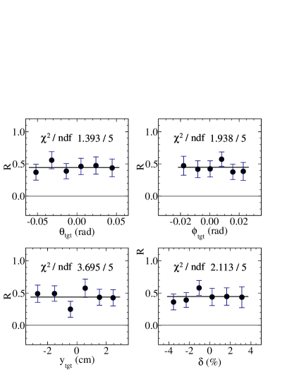
Figure 7: Dependence of extracted $R=\mu_{p}G_{E}^{p}/G_{M}^{p}$ values on the reconstructed proton trajectory parameters at $Q^{2}=4.8$ GeV²: $\theta_{tgt}$ ($\phi_{tgt}$) is the proton trajectory angle relative to the HRS optical axis in the dispersive (non-dispersive) plane, $y_{tgt}$ is the position of the interaction vertex in spectrometer coordinates (see text for details), and $\delta$ is the percentage deviation of the proton momentum from the central HRS momentum setting. In each panel, the data are integrated over the other three variables.

Figure 7 shows the dependence of $R$ at $Q^{2}=4.8$ GeV², extracted using equation (12), on all four proton trajectory parameters that enter the spin transport calculation. These include the trajectory angles $\theta_{tgt}=\tan^{-1}(dx/dz)$ and $\phi_{tgt}=\tan^{-1}(dy/dz)$ relative to the HRS optical axis, the vertex coordinate $y_{tgt}$, defined as the horizontal position of the intersection of the proton trajectory with the plane normal to the HRS optical axis containing the origin, and $\delta\equiv 100\times(p-p_{0})/p_{0}$, the percentage deviation of the measured proton momentum from the HRS central momentum setting. There is no evidence for a dependence of $R$ on any of the variables involved in the precession calculation, indicating the excellent quality of the COSY model. Linear and quadratic fits to the individual dependencies were also performed, and all non-constant terms included in the fits were found to be consistent with zero.

III.2.3 Analyzing Power Calibration

The $\vec{p}+\mbox{CH}_{2}$ analyzing power relating the size of the measured asymmetry to the proton polarization depends on the initial proton momentum and the scattering angle $\vartheta$. Given the relatively small momentum acceptance of the HRS, the $p$-dependence of $A_{y}$ within the acceptance of each $Q^{2}$ point is much weaker than the very strong $\vartheta$ dependence, and can be neglected as a first approximation. Dedicated measurements of $A_{y}$ Azhgirey et al. (2005) at and above the momentum range of the GEp-II experiment were performed prior to the GEp-III experiment. However, precise independent knowledge of $A_{y}$ is not required in the analysis because of the self-calibrating nature of elastic $ep$ scattering, explained below.

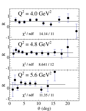
Figure 8: Dependence of the form factor ratio $R$ on the FPP polar scattering angle $\vartheta$ for the three highest $Q^{2}$ values of GEp-II. The constant behavior of $R$ confirms the cancellation of $A_{y}$ in the ratio $P_{t}/P_{\ell}$.

Provided that the effective $\vartheta$ acceptance is $\varphi$-independent, the analyzing power cancels in the ratio $P_{t}/P_{\ell}$ from which the form factor ratio $R$ is extracted, implying that the result for $R$ is independent of $A_{y}$. Uniform $\vartheta$ acceptance is guaranteed by applying a “cone test” in the selection of FPP events, which requires that the projection to the rearmost FPP detector plane of a track originating at the reconstructed $\vec{p}+$CH₂ scattering vertex $z_{close}$ at a polar angle $\vartheta$ falls within the active detector area for all azimuthal angles $\varphi$. Moreover, the cancellation can be verified by binning the results in $\vartheta$ and checking the constancy of $R\propto P_{t}/P_{\ell}$ as a function of $\vartheta$. Figure 8 shows the $\vartheta$ dependence of $R$ for the three highest $Q^{2}$ points of GEp-II. At each $Q^{2}$, a constant fit to the data gives a good $\chi^{2}$ and no systematic trends are observed.

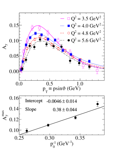
Figure 9: (color online) Top panel: extracted analyzing power as a function of $p\sin\vartheta$, where $p$ is the proton momentum incident on CH₂ (corrected event-by-event for energy loss in CH₂ up to the reconstructed scattering vertex), using the $P_{e}$ values of Table 1, for all four $Q^{2}$ values of the GEp-II experiment. Curves are fits to the data (see text for details). Bottom panel: maximum analyzing power vs. $1/p_{0}$ in GeV^-1, where $p_{0}$ is the central proton momentum, for the four $Q^{2}$ points. Error bars in $A_{y}$ and $A_{y}^{max}$ values are statistical only. See Supplemental Material at Sup for data tables with numerical $A_{y}$ and $A_{y}^{max}$ results.

The fact that $P_{t}$ and $P_{\ell}$ depend only on $R$ and kinematic factors implies that the product $P_{e}A_{y}$ can be extracted by comparing the measured asymmetries $P_{e}A_{y}P_{t}$ and $P_{e}A_{y}P_{\ell}$ to the values of $P_{t}$ and $P_{\ell}$ obtained from equation (I). Combined with the measurements of $P_{e}$ to within an overall accuracy of $\pm 3\%$ by Möller and Compton polarimetery, $A_{y}$ was directly extracted from the data of this experiment. The $p$ and $\vartheta$ dependences of $A_{y}$ thus obtained were then used in equation (12) to improve the statistical precision of the form factor ratio extraction by weighting events according to their analyzing power.

Figure 9 shows the measured $A_{y}$ as a function of the “transverse momentum” $p_{T}\equiv p\sin\vartheta$ for each $Q^{2}$ point, where $p$ is the incident proton momentum corrected for energy loss in CH₂ up to the reconstructed scattering vertex, illustrating the approximate scaling of the angular distribution of $A_{y}$ with momentum. The results shown in Figure 9 are in fairly good agreement with the unpublished results from the original analysis in Gayou (2002), despite using the more restrictive elastic event selection cuts of the present work. This is due in part to the fact that the sensitivity of $P_{\ell}$, from which $A_{y}$ is primarily determined, to $r=G_{E}^{p}/G_{M}^{p}$ is rather weak (see equation (I)). Nonetheless, for the three highest $Q^{2}$ points, the improved suppression of the background in this analysis leads to a slight systematic increase in $A_{y}$, since the asymmetry of the background included in the original analysis partially cancels that of the signal. $A_{y}$ rises rapidly from zero in the region dominated by Coulomb scattering to a maximum at $p_{T}\approx 0.3$ GeV and then tapers off to nearly zero beyond about 1.5 GeV. The measured angular distribution at each $Q^{2}$ was fitted using a simple parametrization $A_{y}(p_{T})=(p_{T}-p_{T}^{0})^{\alpha}e^{-b(p_{T}-p_{T}^{0})^{\beta}}$, where $p_{T}^{0}$, $\alpha$, $b$ and $\beta$ are adjustable parameters. This parametrization incorporates the main features of the angular distribution with sensible limiting behavior and is sufficiently flexible to give a good description of the data. The fit results for each $Q^{2}$ are given in Table 2.

$Q^{2}$ (GeV2)	$p_{T}^{0}$ (GeV)	$\alpha$	$\beta$
3.5	$0.030\pm 0.008$	$0.89\pm 0.06$	$1.19\pm 0.10$
4.0	$0.031\pm 0.003$	$0.88\pm 0.03$	$0.95\pm 0.04$
4.8	$0.029\pm 0.005$	$1.02\pm 0.04$	$1.03\pm 0.05$
5.6	$0.038\pm 0.011$	$1.14\pm 0.09$	$1.12\pm 0.11$
$Q^{2}$ (GeV2)	$b$	$\chi^{2}/\mbox{n.d.f.}$	$A_{y}^{max}$
3.5	$3.51\pm 0.15$	1.23	$0.149\pm 0.005$
4.0	$3.28\pm 0.06$	1.22	$0.123\pm 0.003$
4.8	$3.44\pm 0.06$	1.30	$0.109\pm 0.002$
5.6	$3.67\pm 0.15$	2.02	$0.099\pm 0.004$

Table 2: $A_{y}$ fit results. Parametrization is $A_{y}(p_{T})=\left(p_{T}-p_{T}^{0}\right)^{\alpha}e^{-b\left(p_{T}-p_{T}^{0}\right)^{\beta}}$. The uncertainty in $A_{y}^{max}$ was calculated from the full covariance matrix of the fit result.

The quality of the fit was improved by including the zero offset $p_{T}^{0}$, as the data seem to prefer a vanishing $A_{y}$ at finite $p_{T}^{0}\approx 0.03$ GeV, independent of $Q^{2}$. For $p_{T}<p_{T}^{0}$, $A_{y}=0$ was assumed. The results for the exponents $\alpha$ and $\beta$ are essentially compatible with the product of a linear rise and an exponential decay. An alternate parametrization which fixes $\alpha=1$ and $\beta=1$ and adds an overall normalization constant as a free parameter in addition to the slope parameter $b$ does not describe the data as well as the chosen parametrization in which $\alpha$ and $\beta$ are free parameters but the overall normalization is fixed. The amplitude of the measured $A_{y}$ distribution, as measured by its maximum value, scales approximately with $1/p$, as shown in the bottom panel of Figure 9. Notably, the intercept of the linear fit to the $1/p$ dependence of $A_{y}^{max}$ is compatible with zero, suggesting that the analyzing power for $\vec{p}+\mbox{CH}_{2}$ scattering vanishes for asymptotically large proton momenta, rather than crossing zero at a finite momentum. The fitted curves shown in Figure 9 were used to describe $A_{y}(p_{T})$ in the analysis.

The observed proportionality of $A_{y}$ to $1/p$ allows the momentum dependence of $A_{y}$ to be accounted for in the analysis by simply scaling its value for each event by a factor $p_{0}/p$, where $p_{0}$ is the central proton momentum and $p$ is the proton momentum for the event in question. This is because the fitted $A_{y}(p_{T})$ curve, which is averaged over the $\pm 5\%$ momentum bite of the HRS at each $Q^{2}$, essentially gives $A_{y}(p_{0},p_{T})$, where $p_{0}$ is the central momentum. Assuming that the $1/p$ slope of $A_{y}$ is the same at any $p_{T}$; i.e., assuming a factorized form $A_{y}(p,p_{T})=C(p_{T})/p$, the ratio of $A_{y}(p,p_{T})$ to its known value $A_{y}(p_{0},p_{T})$ at a reference momentum $p_{0}$ is given by $p_{0}/p$, regardless of $C(p_{T})$. While the observed shape of the $p_{T}$ dependence of $A_{y}$ is approximately momentum-independent for the three higher $Q^{2}$ points, the $p_{T}$ dependence of $A_{y}$ at $Q^{2}=3.5$ GeV² is slightly different, with a larger maximum value than suggested by a linear extrapolation from the higher-$Q^{2}$ data and a faster falloff at large $p_{T}$. A plausible, but unproven explanation for the difference in behavior is that the thicker 100 cm analyzer used for the three highest-$Q^{2}$ measurements smears out the $p_{T}$ distribution of both the efficiency and the analyzing power of the FPP relative to the thinner 58 cm analyzer used for the measurement at $Q^{2}=3.5$ GeV². This observation does not, however, invalidate the $p_{0}/p$ scaling of $A_{y}$ in the analysis, because the data from the three higher-$Q^{2}$ points, as well as data from other experiments Punjabi et al. (2005a); Azhgirey et al. (2005), show that the $1/p$ scaling is respected for any given FPP configuration, though the details of $A_{y}(p_{T})$ may differ slightly between different configurations. In any case, the value of $A_{y}$ assigned in the analysis is never changed by more than $\pm 5\%$ for any individual event, so the actual effect of this prescription on the relative weighting of events is rather small.

The description of $A_{y}(p,\vartheta)$ in the present reanalysis differs slightly from that of the original analysis. In this reanalysis, $A_{y}(p,\vartheta)$ is assigned to each event based on the smooth parametrization of $A_{y}(p_{T})$ shown in the curves of Figure 9, which describe the data very well, and an overall $1/p$ scaling. The original analysis, on the other hand, neglected the momentum dependence of $A_{y}$ and assigned $A_{y}(\vartheta)$ to each event based on the calibration results in discrete $\vartheta$ bins. Since $A_{y}$ cancels in the ratio $P_{t}/P_{\ell}$, its description only matters to the extent that it optimizes the statistical precision of the extraction. Different descriptions of $A_{y}(p,\vartheta)$ correspond to different event weights in the analysis, leading to slight differences in the results for $P_{t}$, $P_{\ell}$ and $R$ reflecting statistical fluctuations of the data as a function of $p$ and $\vartheta$. While these differences are always well within the statistical uncertainty of the combined data, better descriptions of $A_{y}(p,\vartheta)$ naturally lead to better overall results.

III.2.4 False Asymmetries

Consistent with the original analysis, no false asymmetry corrections were applied in the present work; i.e., $\lambda_{0}=0$ was assumed in equations (5) and (12). “Weighted sum” estimators, as defined in Besset et al. (1979), can be constructed for the focal plane asymmetries $A_{y}^{FPP}\equiv-P_{e}A_{y}P_{y}^{FPP}$ and $A_{x}^{FPP}\equiv P_{e}A_{y}P_{x}^{FPP}$, equivalent to equation (12) in the absence of precession effects. Including false asymmetry terms up to $2\varphi$, it can be shown that the weighted-sum estimators $\hat{A}_{x}^{FPP}$ and $\hat{A}_{y}^{FPP}$ for the focal plane asymmetries are given to second order in the false and physical asymmetry terms by

$$\hat{A}_{x}^{FPP} = A_{x}^{FPP}\left(1-\frac{c_{2}}{2}\right)-A_{y}^{FPP}\frac{s_{2}}{2}$$

$$\hat{A}_{y}^{FPP} = -\frac{s_{2}}{2}A_{x}^{FPP}+A_{y}^{FPP}\left(1+\frac{c_{2}}{2}\right),$$ (14)

where $c_{2}$ and $s_{2}$ are the false asymmetries as in equation (4). Only the $2\varphi$ Fourier moments of the false asymmetry contribute at this order. The $\cos(2\varphi)$ false asymmetry moment induces a “diagonal” correction to each physical asymmetry term proportional to the asymmetry itself, while the $\sin(2\varphi)$ false asymmetry moment induces an “off-diagonal” correction to $A_{x}^{FPP}$ ($A_{y}^{FPP}$) proportional to $A_{y}^{FPP}$ ($A_{x}^{FPP}$).

Fourier analysis of the helicity sum distribution $n_{+}+n_{-}$ showed that the acceptance-averaged magnitude of $c_{2}$ and $s_{2}$ did not exceed $2.5\times 10^{-3}$ at any $Q^{2}$, and neither term exceeded $1\%$ at any $\vartheta$ within the useful range. The possible effect of $c_{2}$ on the “diagonal” terms is therefore at the $10^{-3}$ (relative) level, while the “off-diagonal” correction is at the $10^{-5}$ level (absolute) for the small $A_{y}^{FPP}$ term, and even smaller for the larger $A_{x}^{FPP}$ term. Compared to both the size and statistical uncertainty in the asymmetries (see Fig. 6), and the systematic uncertainties in $P_{t}$ and $P_{\ell}$ resulting from the spin transport calculation, such corrections are completely negligible. This is in contrast to the GEp-III and GEp-2$\gamma$ analyses, in which a sizeable $\cos(2\varphi)$ false asymmetry in the Hall C FPP induced a correction that, while small, made a non-negligible contribution to the total systematic uncertainty.

III.3 Background Estimation and Subtraction

From Figure 5, two qualitative features of the data are obvious. First, the non-elastic background before applying two-body correlation cuts is substantial. Second, examination of the $\Delta x$ and $\Delta y$ spectra before and after applying the $\delta p$ cut reveals that the $\delta p$ cut provides significant additional background suppression power relative to $\Delta x$ and $\Delta y$ cuts alone, with minimal reduction of the elastic peak strength, implying that events outside the $\delta p$ cut are background-dominated, even after calorimeter cuts.

As alluded to in sections II.2 and III.1, the non-elastic background for the measurements using a calorimeter for electron detection consists predominantly of two reactions, quasi-elastic Al($e,e^{\prime}p$) scattering in the cryocell entrance and exit windows, and $\pi^{0}$ production initiated by the flux of real Bremsstrahlung photons radiated along the target material (photoproduction) as well as virtual photons present in the electron beam independent of target thickness (electroproduction). Due to the kinematic acceptance of the experiment and the $Q^{2}$ dependence of the respective cross sections, the contribution of $\pi^{0}p$ electroproduction is mostly limited to “quasi-real” photons; i.e., $Q^{2}\approx 0$, and is practically indistinguishable from real photoproduction. By detecting both scattered particles in coincidence, the two-body $ep\rightarrow ep$ kinematics are overdetermined, providing for a clean selection of elastic events and a direct determination of the remaining background from the data, with no external inputs, using the sideband-fitting method described in section III.3.2 below. The main disadvantage of this approach to background estimation is that it makes no reference to the underlying physics of the signal and background. For this reason, a Monte Carlo simulation of the experiment was carried out to confirm the conclusions regarding backgrounds obtained directly from the data. However, the results of the simulation were not used in any way as input to the final analysis.

III.3.1 Monte Carlo Simulation

The simulation code is the same as that used in the data analysis of Qattan et al. (2005), which already includes a realistic model of the HRSL. Modifications of the code used in the analysis of Ref. Qattan et al. (2005) to reproduce non-Gaussian tails of the HRS resolution, caused by multiple scattering and other effects, were not included here. The only significant addition to the code was a description of the acceptance and resolution of the GEp-II calorimeter. Because the $15\times 15$ cm² cell size of the GEp-II calorimeter is large compared to the Moliére radius of lead-glass, coordinate reconstruction essentially consists of assigning the shower coordinates to the center of the cell with maximum energy deposition. Furthermore, the discriminator threshold applied to form the timing signal was roughly 20% of the elastically scattered electron energy, meaning that signals below this amplitude would be rejected in software by the timing cut. The electron energy and coordinates were thus defined by the signal in a single block in the overwhelming majority ($\gtrsim 90\%$) of elastic events. Physics ingredients of the simulation include cross section models for ¹H$(e,e^{\prime}p)$, Al$(e,e^{\prime}p)$ and ¹H$(\gamma,\pi^{0}p)$ reactions, a realistic calculation of the Bremsstrahlung flux for $\pi^{0}$ photoproduction, and event-by-event radiative corrections to the $(e,e^{\prime}p)$ cross sections following the approach of Ent et al. (2001), providing for a rigorous deconvolution of the signal and background contributions to the $\Delta x$, $\Delta y$, and $\delta p$ distributions for arbitrary cuts. Another reaction that can contribute to the background is Real Compton Scattering $\gamma p\rightarrow\gamma p$ (RCS), whose end-point kinematics are identical to $ep\rightarrow ep$. However, the cross section for this reaction is generally much smaller than for $\pi^{0}$ photoproduction Danagoulian et al. (2007); Shupe et al. (1979), and was neglected.

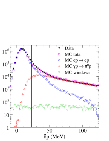
Figure 10: (color online) Contributions to the $\delta p$ distribution at $Q^{2}=4.8$ GeV² estimated from the Monte Carlo simulation. Monte Carlo distributions are shown for elastic $ep$ (empty circles), $\gamma p\rightarrow\pi^{0}p$ (empty triangles), and quasi-elastic $(e,e^{\prime}p)$ in the target windows (empty inverted triangles). The sum of all Monte Carlo contributions (empty squares) is compared to the data of Figure 5(c) (solid inverted triangles). Monte Carlo and data distributions are obtained after applying $\Delta x$ and $\Delta y$ (calorimeter) cuts. Black vertical lines show the $\delta p$ cut region of the final analysis. Uncertainties shown are statistical only. See text for details.

Figure 10 shows the simulated $\delta p$ distribution in the vicinity of the elastic peak for each reaction considered, after applying $\Delta x$ and $\Delta y$ cuts. As described below, the simulated target window yield was normalized to match the window yield obtained from the data in the super-elastic ($\delta p<0$) region. Then, the overall normalization constants for $\pi^{0}p$ and elastic $ep$ events were fitted simultaneously to minimize the statistics-weighted sum of squared differences between the data and the sum of Monte Carlo yields. The agreement between data and Monte Carlo is good, but not perfect, primarily because non-Gaussian tails are not included in the simulated $\delta p$ resolution. Nonetheless, the $\delta p$ distribution after cuts is described to within $\sim 20\%$ in the relevant $\delta p$ range, with the exception of disagreements of up to $\sim 40\%$ in the $\delta p$ region from 20-40 MeV just above the elastic peak, which is rather sensitive to non-Gaussian tails and the details of the Bremsstrahlung spectrum and the $\pi^{0}$ production cross section near end-point. Since the purpose of the simulation was to provide a qualitative illustration of the physics of the signal and the background, and since the background contamination and its polarization were determined directly from the data for the final analysis, no additional fine-tuning of the simulation was attempted.

Two key features of the simulation results deserve special emphasis. First, the contribution of the $ep$ radiative tail in the inelastic region falls off too quickly to describe the observed tail of the data. This is a consequence of the $\Delta x$ cut, with $\Delta x$ calculated using the GEp-II method Gayou (2002). The background fraction exceeds 80% above 50 MeV and 90% above 75 MeV. The $ep$ yield falls below the $\pi^{0}p$ yield at $\sim$40 MeV and becomes negligible above $\sim 120$ MeV, confirming the conclusion that the inelastic region of the $\delta p$ distribution is dominated by the $\pi^{0}p$ background rather than the $ep$ radiative tail. Second, the target window contribution is vanishingly small compared to the elastic and $\pi^{0}p$ contributions in the entire $\delta p$ range of interest. More specifically, in the region below $\pi^{0}$ threshold, the window contribution is the dominant component of the background, but is too small relative to the elastic yield to affect the measured asymmetry, while in the region where the contamination is sufficiently large to affect the asymmetry, the $\pi^{0}$ contribution is dominant. Moreover, the proton recoil polarization in quasi-elastic Al$(\vec{e},e^{\prime}\vec{p})$ scattering at high $Q^{2}$ should be similar, in principle, to that in elastic $\vec{e}p\rightarrow e\vec{p}$, since the former process is simply the latter process embedded in a nucleus, whereas the spin structure of $\vec{\gamma}p\rightarrow\pi^{0}\vec{p}$ can be (and is) dramatically different.

The only kinematically allowed reactions producing protons in the super-elastic region are quasi-elastic Al$(e,e^{\prime}p)$ and other reactions occurring on the Al nuclei in the cryocell windows, in which the initial Fermi motion of the struck proton can lead to proton knockout with $p_{p}>p_{p}(\theta_{p})$. However, a significant fraction of the yield in the super-elastic region actually comes from hydrogen, because the combined thickness of the entrance and exit windows of the Hall A cryotarget Alcorn et al. (2004) in g cm^-2 is only about 4% of the liquid hydrogen thickness, and the non-Gaussian tails of the $\delta p$ resolution smear a fraction of hydrogen events into the unphysical $\delta p$ region. The reconstructed vertex distribution in this region exhibits narrow peaks at the window locations and a smooth hydrogen background extending over the full target length. To estimate the yield from the target windows, the vertex $z$ distribution was plotted as a function of $\delta p$ in the super-elastic region for events failing the $\Delta x$ and $\Delta y$ cuts, in order to enhance the very small window “signal” relative to the large hydrogen elastic “background”. For each of six $\delta p$ bins in $-180\leq\delta p\mbox{ (MeV)}\leq 0$, a polynomial fit to the smooth hydrogen background was subtracted from the vertex $z$ distribution, leaving only the window peaks. For each window, the simulated $\delta p$ distribution with identical cuts applied was normalized to match the background-subtracted window yield obtained from the data. The resulting normalization factor was then applied to the simulated $\delta p$ distribution of window events passing the $\Delta x$ and $\Delta y$ cuts, leading to the contribution shown in Fig. 10.

Given the vertex resolution of the HRS, a vertex cut chosen to exclude the windows at the $3\sigma$ level can further suppress the very small window background, at the expense of a $\sim$20% reduction in elastic $ep$ statistics. However, the aforementioned analysis of the window yield suggests that even when the full target length is included, the fraction of the total yield from the windows is negligible after all cuts are applied, making additional vertex cuts unnecessary. This conclusion is further supported by comparing the $\delta p$ distributions with and without such a vertex cut, and by comparing the $\delta p$ spectra for the $Q^{2}\geq 4.0$ GeV² settings to the $\delta p$ spectrum of the $Q^{2}=3.5$ GeV² setting, for which the precise measurement of the electron kinematics with a magnetic spectrometer provides an essentially background-free selection of elastic events, as discussed in Section II.1.2. Based on these considerations, the window contamination was deemed negligible, and the study of the background contamination focused mainly on the inelastic ($\delta p>0$) region.

The background subtraction procedure used for the final analysis is agnostic regarding the reaction mechanism responsible for the contamination, with the caveat that the conclusion of negligible window contamination is used to justify the assumption of constant background polarization, which reduces the statistical uncertainty in the background correction. In summary, the simulation provides a qualitative description of the data that supports the conclusions of this analysis regarding backgrounds. Averaged over the final $\delta p$ cut region, the fractional background contamination obtained from the simulation agrees with that obtained directly from the data at a level similar to its systematic uncertainty, which is determined by the data.

III.3.2 Sideband subtraction

For the final analysis, the fractional background contamination in the sample of elastic $ep$ events selected by a given set of cuts was estimated by fitting the tails of the $\Delta x$ and $\Delta y$ distributions on either side of the elastic peak and extrapolating into the peak region, as shown in Figures 5(a) and 5(b). This approach to background estimation implies two assumptions. First, the contribution of elastic scattering to the tails of the $\Delta x$ and $\Delta y$ distributions is assumed to be negligible for values of $\Delta x$ and $\Delta y$ sufficiently far away from the elastic peak. Second, the background is assumed to have a smooth distribution under the elastic peak, so that joining the tails with a smooth interpolating function is a good approximation to the true background shape. The first assumption can in principle be violated by the $ep$ radiative tail and by non-Gaussian smearing effects in the HRS angle and momentum reconstruction. Radiation redistributes elastic $ep$ events away from the elastic peak toward negative $\Delta x$ values, but does not markedly affect the $\Delta y$ distribution of elastic events, since $\Delta y$ reflects the extent to which the two detected particles are non-coplanar, and the coplanarity of outgoing particles is not strongly affected by radiation. Furthermore, the $\delta p$ cut suppresses the radiative tail of the $\Delta x$ distribution. Non-Gaussian smearing effects do not contribute a significant fraction of events in the tails except when the background contribution is very small. The second assumption (smooth background distribution) was confirmed by inspecting the correlations between $\Delta x$ and $\Delta y$; i.e., by plotting $\Delta x$ ($\Delta y$) for $\Delta y$ ($\Delta x$) well outside the elastic peak. This assumption was also supported by the simulations described in section III.3.1. Although the simulation does not include the contribution of random coincidences, the contamination of the data by random coincidences is negligible after timing and kinematic cuts.

In the following discussion, the fractional background contamination $f$ is defined as $f\equiv B/(S+B)$, where $B$ is the number of background events and $S$ is the number of signal events; i.e., $f$ is the ratio of the background yield to the total yield. The value of $f$ and its systematic uncertainty $\Delta f$ were estimated using a conservative approach involving a total of twelve different fits. The tails of the $\Delta x$ and $\Delta y$ distributions, obtained after applying all other cuts, were each fitted with Gaussian and polynomial background shapes, for three different sizes of the elastic peak region excluded from the fit (two spectra $\times$ two parametrizations $\times$ three sideband ranges $=$ twelve fits). The average fit result was taken as the value of $f$, while the rms deviation of the fit result from the mean was taken as the systematic uncertainty $\Delta f$. The variations among the different fit results reflect the level of agreement (or disagreement) among the different spectra, assumed background lineshapes, and regions excluded from the fit.

A central conclusion of the present reanalysis is that the background was underestimated in the original analysis. Using the polynomial sideband fitting method, the estimated average values of $f$ for the cuts of the original analysis, in which no $\delta p$ cut was applied, are 1.6%, 2.8% and 5.3% for $Q^{2}=4.0$, 4.8 and 5.6 GeV², respectively. Compared to the estimates reported in Gayou (2002) for the original analysis, these estimates are higher by factors of 2.3, 7.0 and 3.8, respectively. Even at the few percent level, neglected or underestimated inelastic contamination can have a non-negligible effect on the measured asymmetries if the polarization of the background differs strongly enough from that of the signal, as in this case.

With the addition of the $\delta p$ cut, the present analysis maximally exploits the two-body kinematic correlations of both detected particles. In the inelastic region, $\pi^{0}$ production dominates. In terms of $\delta p$, the $\pi^{0}$ production “threshold” is very close to the elastic peak. When reconstructed assuming elastic scattering, protons from $\gamma p\rightarrow\pi^{0}p$ at the Bremsstrahlung end-point have $\delta p=7.4$, 8.1 and 8.8 MeV for $Q^{2}=$ 4.0, 4.8 and 5.6 GeV², respectively. When compared to the $\delta p$ resolution of $\sim 5$ MeV, there is clearly substantial overlap of the $\pi^{0}p$ kinematic phase space with the elastic peak, as in the example of Figure 10. As $Q^{2}$ increases at a given beam energy, the $\pi^{0}p$ cross section becomes large compared to the $ep$ cross section.

The effect of underestimating the $\pi^{0}$ background on the form factor ratio extraction is illustrated in Figure 11, which shows $P_{t}$, $P_{\ell}$ and $f$ as a function of $\delta p$, for events identified as elastic in the original analysis, at $Q^{2}=4.8$ GeV².

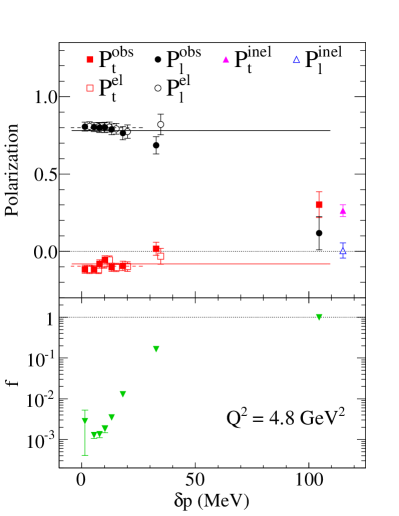
Figure 11: (color online) Top panel: $\delta p$ dependence of $P_{t}$ and $P_{\ell}$ for events selected by the $\Delta x$ and $\Delta y$ cuts of Figure 5. Data are binned in $\delta p$ as described in the text and plotted at the average $\delta p$ value in each bin. Raw polarizations $P_{t}^{obs}$ (filled squares) and $P_{\ell}^{obs}$ (filled circles) approach the background polarizations $P_{t}^{inel}$ (filled triangle) and $P_{\ell}^{inel}$ (empty triangle) at large $\delta p$. Corrected values $P_{t}^{el}$ (empty squares) and $P_{\ell}^{el}$ (empty circles) are offset in $\delta p$ for clarity. Dashed and solid horizontal lines are weighted averages of the corrected and raw data, respectively. Bottom panel: $\delta p$ dependence of the fractional background contamination $f$. Uncertainties in $f$ are systematics-dominated, while the uncertainties in the polarization components are statistics-dominated. See text for details.

The data were divided into eight $\delta p$ bins, including six equal-statistics bins inside the cut region of Figure 5(c), where $f$ is very small ($-7.3\leq\delta p\leq 22.7$ MeV), a seventh bin with a significant fraction of both signal and background ($22.7\leq\delta p\leq 60$ MeV), and an eighth bin dominated by background ($\delta p>60$ MeV). Because the $\Delta x$ and $\Delta y$ distributions in the last $\delta p$ bin showed no obvious signature of an elastic peak, $f=1$ was assumed for this bin, consistent with the simulation results shown in Figure 10. Meaningful background estimation and subtraction were not possible for this bin. As $\delta p$ increases, the raw transferred polarization components $P_{t}^{obs}$ and $P_{\ell}^{obs}$ evolve from their roughly constant values in the signal-dominated region to values that are consistent with the background polarization components $P_{t}^{inel}$ and $P_{\ell}^{inel}$. The $\delta p$-integrated results for the background polarization, extracted from events rejected by the cuts of Figure 5, are plotted at an arbitrary $\delta p=115$ MeV for comparison.

The background polarization components were obtained by applying anti-cuts twice as wide as the final elastic event selection cuts; i.e., $\Delta x$($\Delta y$) was required to be at least 24(32) cm away from the midpoint between half-maxima of the peak. Events selected by this anticut are background-dominated and have negligible elastic contamination. In order to study the $\delta p$ dependence of $P_{i}^{inel}$, no cut was applied to $\delta p$ in the extraction of the background polarization. No statistically significant $\delta p$ dependence of the background polarization was observed, consistent with dominance of the background by $\pi^{0}p$ events. Therefore, $P_{i}^{inel}$ was assumed constant in the background subtraction procedure.

In Figure 11, the signal polarization $P_{i}^{el}(i=t,\ell)$ was obtained from $P_{i}^{obs}$ in the first seven bins using the subtraction

$$P_{i}^{el}=\frac{P_{i}^{obs}-fP_{i}^{inel}}{1-f}.$$ (15)

By comparing the weighted average of all uncorrected data in Figure 11 to the weighted average of the six corrected data points inside the cut region, it is found that the background contamination of the sample with no $\delta p$ cut induces relative systematic shifts of $\left|\Delta P_{t}/P_{t}\right|=15.8\%$ and $\left|\Delta P_{\ell}/P_{\ell}\right|=2.4\%$. From Figure 11, it is clear that the tails of the $\delta p$ distribution outside the cut region of Figure 5(c) contribute very little to the statistical precision of the measurement of $P_{t}/P_{\ell}$ while causing a large systematic effect. For the final analysis, rather than correcting the results bin-by-bin in $\delta p$ using equation (15), as in Figure 11, the background fraction $f$ and polarization $P_{i}^{inel}$ were included at the individual event level in equation (12) by making the following replacements:

$$\lambda_{t,\ell}^{(i)} \rightarrow \lambda_{t,\ell}^{(i)}(1-f_{i})$$

$$\left(1-\lambda_{0}^{(i)}\right) \rightarrow \left(1-\lambda_{0}^{(i)}-\lambda_{inel}^{(i)}\right),$$ (16)

where $f_{i}$ is the background contamination as a function of $\delta p^{(i)}$ and $\lambda_{inel}^{(i)}$, representing the background asymmetry, is given by

$$\lambda_{inel}^{(i)} \equiv f_{i}h_{i}P_{e}A_{y}^{(i)}\left[\left(S_{xt}^{(i)}\cos\varphi_{i}-S_{yt}^{(i)}\sin\varphi_{i}\right)P_{t}^{inel}+\right.$$ (17)

$$\left.\left(S_{x\ell}^{(i)}\cos\varphi_{i}-S_{y\ell}^{(i)}\sin\varphi_{i}\right)P_{\ell}^{inel}\right].$$

This method is functionally equivalent to correcting the results “after the fact” using equation (15). It also simplifies the evaluation of systematic uncertainties associated with the background correction, which were obtained by varying $f$, $P_{t}^{inel}$ and $P_{\ell}^{inel}$ within their uncertainties and observing the shift in $R$.

III.4 Systematic Uncertainties

As a result of the cancellation of the beam polarization and analyzing power in the ratio $P_{t}/P_{\ell}$ and the cancellation of the FPP instrumental asymmetry by the beam helicity reversal, there are few significant sources of systematic uncertainty in the results of this experiment (as is also the case in the GEp-I, GEp-III and GEp-2$\gamma$ experiments). The dominant source of systematic uncertainty is the spin transport calculation. Since the procedure for the evaluation of systematic uncertainties associated with this calculation is documented at length in Refs. Pentchev and LeRose (2001); Pentchev (2003); Punjabi et al. (2005a); Gayou (2002), only a brief summary of the studies and the conclusions is given here.

The range of non-dispersive plane trajectory bend angles $\phi_{bend}$ accepted by the HRS is roughly $\pm 60$ mrad, independent of momentum. The maximum accepted range of the non-dispersive plane precession angle $\chi_{\phi}=\gamma\kappa_{p}\phi_{bend}$ is roughly $\pm 30^{\circ}$ at the highest $Q^{2}$ of 5.6 GeV². To first order in $\chi_{\phi}$, the ratio $P_{t}/P_{\ell}$ is given in terms of the focal plane ratio $P_{y}^{FPP}/P_{x}^{FPP}$ by $P_{t}/P_{\ell}\approx\chi_{\phi}-\sin\chi P_{y}^{FPP}/P_{x}^{FPP}$. Because the non-dispersive plane precession mixes $P_{t}$ and $P_{\ell}$, the ratio is highly sensitive to uncertainties in $\phi_{bend}$. To first order, an uncertainty $\Delta\phi_{bend}$ leads to an uncertainty $\Delta R\approx\left(\mu_{p}\sqrt{\tau(1+\epsilon)/2\epsilon}\right)\gamma\kappa_{p}\Delta\phi_{bend}$ in the extracted form factor ratio. The error magnification factor multiplying $\Delta\phi_{bend}$ grows as large as 33 at $Q^{2}=5.6$ GeV². To manage the systematic uncertainty due to the precession calculation, $\phi_{bend}$ must be known to very high accuracy. On the other hand, since $\theta_{bend}$ only enters $P_{t}/P_{\ell}$ through the factor of $\sin\chi$ multiplying $P_{y}^{FPP}/P_{x}^{FPP}$, and since the reconstruction of $\theta_{bend}$ involves relatively small deviations about the 45^∘ central bend angle, the accuracy of $P_{t}/P_{\ell}$ is far less sensitive to systematic errors in $\theta_{bend}$ and $p_{p}$.

The major sources of uncertainty in $\phi_{bend}$ are horizontal misalignments and rotations of the three quadrupoles relative to the HRSL optical axis defined by the dipole magnet. In order to control the uncertainty in $\phi_{bend}$ to the highest possible accuracy, dedicated studies of the optical properties of HRSL in the non-dispersive plane were performed. Electrons were scattered from a thin carbon foil aligned with the HRSL optical axis, and a special “sieve-slit” collimator was installed in front of the entrance to HRSL before the first quadrupole magnet. The sieve-slit collimator, part of the standard equipment of the HRSs, consists of a 5 mm thick stainless steel sheet with a pattern of 49 holes ($7\times 7$), spaced 25 mm apart vertically and 12.5 mm apart horizontally, used for optics calibrations Alcorn et al. (2004). In the studies described here, electrons passing through the central sieve hole aligned with the HRS optical axis were selected. For a series of deliberate mistunings of the HRS quadrupoles relative to the nominal tune, the displacements in both position and angle of the image of the central sieve hole at the focal plane were observed. Combined with the known first-order HRS optics coefficients describing the effects of quadrupole misalignments and rotations, the information gained from these studies placed a much more stringent constraint on the misalignments than the nominal accuracy of the quadrupole positions. By reducing the uncertainty $\Delta\phi_{bend}$ to $\pm$0.3 mrad, the optical studies reduced the systematic uncertainty in $R$ at $Q^{2}=5.6$ GeV², where the result is most sensitive to $\phi_{bend}$, to a level comparable with other contributions.

Additional model uncertainties in the precession calculation due to the field layout in COSY are more difficult to quantify, but are typically smaller than the errors associated with the accuracy of the inputs to the calculation; i.e., the reconstructed proton kinematics. The COSY model uncertainties were estimated by performing the calculation in several different ways. For the final analysis, the proton trajectory angles, momentum and vertex coordinates, calculated using the standard HRS optics matrix tuned to calibration data as described in Alcorn et al. (2004), were used to calculate the forward spin transport matrix, as described in section III.2.2. To estimate systematic uncertainties, the calculation was also performed using the same forward spin transport matrix, but the kinematics were reconstructed using an alternate set of optics matrix elements calculated by COSY. Finally, COSY was used to calculate the expansion of the reverse spin transport matrix, which was then inverted to obtain the forward matrix elements that enter the likelihood function of equation (5). A model systematic uncertainty was assigned based on the variations in the results among the different methods, as described in Gayou (2002).

Apart from the uncertainties associated with the non-elastic background, which were underestimated by the original analysis, the main additional source of uncertainty is the accuracy of the scattering angle reconstruction in the FPP. Uncertainties associated with FPP reconstruction were minimized by a software alignment procedure using “straight-through” data obtained with the CH₂ analyzers removed. The systematic errors in $R$ due to the absolute accuracy in the determination of the beam energy ($\delta E/E\sim 2\times 10^{-4}$) and the proton momentum ($\delta p/p\sim 4\times 10^{-4}$) Alcorn et al. (2004), which mainly enter the ratio $R$ through the kinematic factor $\mu_{p}\sqrt{\tau(1+\epsilon)/2\epsilon}$ of equation (I), are negligible compared to the precession-related uncertainties.

The updated systematic uncertainties associated with the background estimation and subtraction procedure are very small as a result of the added $\delta p$ cut, and are generally at the $10^{-3}$ level. The “Bckgr.” uncertainty in Table 3 was obtained by varying $f$, $P_{t}^{inel}$ and $P_{\ell}^{inel}$ within their uncertainties, which are systematics-dominated for $f$ and statistics-dominated for $P_{i}^{inel}$, and observing the shift in $R$. The contributions from $f$ and $P_{t}^{inel}$ are comparable, while the contribution from $P_{\ell}^{inel}$ is much smaller.

The present analysis also examined the sensitivity of $R$ to variations in elastic event selection cuts. The analysis was performed for various $\Delta x$, $\Delta y$ and $\delta p$ cut widths, using both the GEp-II and GEp-III definitions of $\Delta x$ and $\Delta y$ (see section III.1). The analysis was also performed using the original polygon cut, supplemented by the new $\delta p$ cut. For consistency of background corrections, the contamination was estimated separately for each case. The rms variation of $R$ due to cut variations is quoted as the “Cuts” uncertainty of Table 3. It is generally larger than the “Bckgr.” uncertainty calculated using the final cuts, and reflects fluctuations among slightly different selections of events, not necessarily related to the background. It is, however, much smaller than the statistical uncertainty at each $Q^{2}$.

The present reanalysis of the GEp-II data is identical to the original analysis in event reconstruction, spin transport calculations, and all cuts other than $\Delta x$, $\Delta y$ and $\delta p$ used to select elastic events. The only other meaningful difference between the present reanalysis and the original analysis is the improved description of the analyzing power discussed in section III.2.3, which only affects the results through slight modification of the $p$ and $\vartheta$-dependent weighting of events. Therefore, aspects of systematic uncertainty analysis other than elastic event selection and background subtraction were not revisited. These aspects of the analysis are documented at length in Gayou (2002).

Table 3: Total systematic uncertainty in $R$ and its contributions. See text for details.

$Q^{2}$, GeV2	3.5	4.0	4.8	5.6
$\vartheta_{FPP}$	$1.4\times 10^{-3}$	$0.8\times 10^{-3}$	$1.4\times 10^{-3}$	$0.7\times 10^{-3}$
$\varphi_{FPP}$	$5.1\times 10^{-3}$	$6.3\times 10^{-3}$	$6.1\times 10^{-3}$	$2.9\times 10^{-3}$
$\theta_{bend}$	$4.6\times 10^{-3}$	$0.1\times 10^{-3}$	$2.6\times 10^{-3}$	$4.3\times 10^{-3}$
$\phi_{bend}$	$1.3\times 10^{-3}$	$1.1\times 10^{-3}$	$6.1\times 10^{-3}$	$12.3\times 10^{-3}$
COSY	$0.4\times 10^{-3}$	$0.4\times 10^{-3}$	$1.2\times 10^{-3}$	$12.7\times 10^{-3}$
Bckgr.	N. A.	$0.9\times 10^{-3}$	$1.1\times 10^{-3}$	$1.2\times 10^{-3}$
Cuts	N. A.	$5.4\times 10^{-3}$	$7.2\times 10^{-3}$	$3.9\times 10^{-3}$
Total	$7.0\times 10^{-3}$	$8.5\times 10^{-3}$	$11.7\times 10^{-3}$	$18.9\times 10^{-3}$

Table 3 shows all known contributions to the systematic uncertainty in $R$ at each $Q^{2}$, including the polar ($\vartheta_{FPP}$) and azimuthal ($\varphi_{FPP}$) angle reconstruction in the FPP, the dispersive ($\theta_{bend}$) and non-dispersive ($\phi_{bend}$) trajectory bend angles, the COSY model uncertainty (COSY), the non-elastic background contribution (Bckgr.) and the cut sensitivity (Cuts). All contributions are added in quadrature to obtain the total systematic uncertainty. Uncertainties due to FPP instrumental asymmetries are negligible as discussed in section III.2. In the final analysis of the GEp-II experiment, the total accuracy of the results is statistics-limited, with systematic uncertainties at a much lower level.

As in the original publication Gayou et al. (2002), no radiative corrections have been applied to the data presented here. Standard, model-independent radiative corrections to $R$ were calculated in Afanasev et al. (2001) for kinematics very close to those of the GEp-II experiment and found to be less than 1% (relative) for all four $Q^{2}$ values. Though even 1% relative corrections are much smaller than the statistical uncertainties in the data, the calculations in Afanasev et al. (2001) were performed assuming a much wider “inelasticity” cut than that effected by the combination of cuts applied in the present analysis, such that in reality, the standard radiative corrections to the GEp-II data are even smaller, which justifies neglecting them here.

IV Results

IV.1 Discussion of the Data

Table 4: Final results of the GEp-II experiment. $\left<Q^{2}\right>$ is the acceptance-averaged $Q^{2}$, while $\Delta Q^{2}$ is the half-width of the total $Q^{2}$ interval, which is centered at the nominal $Q^{2}$. The raw ($P_{i}^{obs}$), background ($P_{i}^{inel}$) and corrected ($P_{i}^{el}$) polarization transfer components and the raw form factor ratio $R$ are presented with statistical uncertainties only. The background fraction $\left<f\right>$ averaged over the final cut region is quoted with its systematic uncertainty $\Delta f$. The final results for $R=\mu_{p}G_{E}^{p}/G_{M}^{p}$ are quoted with statistical and systematic uncertainties. The data at $Q^{2}=3.5$ GeV² were not reanalyzed, and the quoted result is identical to that of the original publication Gayou et al. (2002). The originally published results Gayou et al. (2002) are quoted on the bottom line for comparison.

Nominal $Q^{2}$ (GeV2)	3.5	4.0	4.8	5.6
$\left<Q^{2}\right>\pm\Delta Q^{2}$ (GeV2)	$3.50\pm 0.23$	$3.98\pm 0.26$	$4.76\pm 0.30$	$5.56\pm 0.34$
$P_{t}^{obs}\pm\Delta P_{t}^{obs}$	N. A.	$-0.108\pm 0.011$	$-0.094\pm 0.011$	$-0.070\pm 0.017$
$P_{\ell}^{obs}\pm\Delta P_{\ell}^{obs}$	N. A.	$0.683\pm 0.012$	$0.795\pm 0.013$	$0.886\pm 0.030$
$R\pm\Delta R$ (raw)	N. A.	$0.514\pm 0.055$	$0.445\pm 0.052$	$0.350\pm 0.085$
$\left<f\right>\pm\Delta f$	N. A.	$(0.30\pm 0.04)\%$	$(0.38\pm 0.06)\%$	$(0.47\pm 0.07)\%$
$P_{t}^{inel}\pm\Delta P_{t}^{inel}$	N. A.	$0.116\pm 0.051$	$0.264\pm 0.038$	$0.128\pm 0.034$
$P_{\ell}^{inel}\pm\Delta P_{\ell}^{inel}$	N. A.	$0.224\pm 0.053$	$0.006\pm 0.049$	$0.278\pm 0.072$
$P_{t}^{el}\pm\Delta P_{t}^{el}$	$-0.118\pm 0.015$	$-0.109\pm 0.011$	$-0.096\pm 0.011$	$-0.071\pm 0.017$
$P_{\ell}^{el}\pm\Delta P_{\ell}^{el}$	$0.616\pm 0.017$	$0.685\pm 0.012$	$0.799\pm 0.013$	$0.890\pm 0.030$
$R\pm\Delta R_{stat}\pm\Delta R_{syst}$ (final)	$0.571\pm 0.072\pm 0.007$	$0.517\pm 0.055\pm 0.009$	$0.450\pm 0.052\pm 0.012$	$0.354\pm 0.085\pm 0.019$
$P_{t}\pm\Delta P_{t}$ (equation (I))	$-0.118\pm 0.014$	$-0.109\pm 0.011$	$-0.096\pm 0.011$	$-0.071\pm 0.017$
$P_{\ell}\pm\Delta P_{\ell}$ (equation (I))	$0.616\pm 0.005$	$0.685\pm 0.003$	$0.799\pm 0.002$	$0.890\pm 0.002$
$R\pm\Delta R_{stat}\pm\Delta R_{syst}$ (Gayou et al. (2002))	$0.571\pm 0.072\pm 0.007$	$0.482\pm 0.052\pm 0.008$	$0.382\pm 0.053\pm 0.011$	$0.273\pm 0.087\pm 0.028$

The final results of the GEp-II experiment are reported in Table 4 and presented in Figure 12.

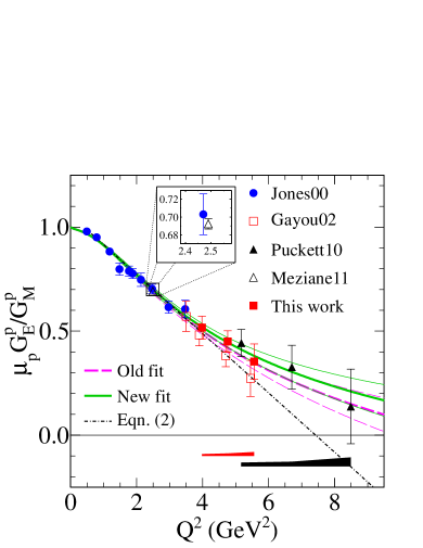
Figure 12: (color) Polarization transfer data for $G_{E}^{p}/G_{M}^{p}$ from Punjabi et al. (2005a) (Jones00), Gayou et al. (2002) (Gayou02), Puckett et al. (2010) (Puckett10), Meziane et al. (2011) (Meziane11) and the present work. Error bars are statistical. The data of Gayou et al. (2002) are offset slightly in $Q^{2}$ for clarity. Systematic uncertainties for the present work and Puckett et al. (2010) are shown as bands below the data. The inset shows a zoomed view of the data near $Q^{2}=2.5$ GeV², demonstrating the excellent agreement between high-precision data from Hall A Punjabi et al. (2005a) and Hall C Meziane et al. (2011) at this $Q^{2}$. Curves are global proton form factor fits using the originally published GEp-II data Gayou et al. (2002) (Old fit) and the present work (New fit), with standard $1\sigma$ point-wise uncertainty bands. Both fits include the GEp-III data. The linear fit of equation (2) is shown for comparison. See text for details.

The values and statistical uncertainties of $P_{t}^{el}$ and $P_{\ell}^{el}$ presented in Table 4 (and Figure 11) are obtained from equation (12). Because the analyzing power is calibrated using equation (I), the extracted $P_{t}^{el}$ and $P_{\ell}^{el}$ values are, by definition, equal to those of equations (I), which depend only on $R$ and kinematic factors, regardless of the value of $P_{e}$ assumed in the analysis. For reference, the values of $P_{e}$ used in the analysis at each $Q^{2}$ are shown in Table 1. These values are based on the average of all beam polarization measurements at a given setting. Because $P_{e}$ was stable at the few percent level throughout the duration of each kinematic setting, a single $P_{e}$ value was assigned to all data taken at a given $Q^{2}$. As presented, the statistical uncertainties in $P_{t}^{el}$ and $P_{\ell}^{el}$ correspond to the uncertainties in the raw asymmetries measured by the FPP, which are large compared to the corresponding systematic uncertainties.

$P_{t}$ and $P_{\ell}$ can also be calculated from $R$ and kinematic factors using equation (I). Neglecting the very small covariance of $P_{t}$ and $P_{\ell}$ and the uncertainty in the kinematic factors involved, the uncertainty in $R$ is given by $\left(\Delta R/R\right)^{2}=\left(\Delta P_{t}/P_{t}\right)^{2}+\left(\Delta P_{\ell}/P_{\ell}\right)^{2}$. While the uncertainties in $P_{t}$ and $P_{\ell}$ obtained from equation (12) are similar, and $\Delta P_{\ell}^{el}$ is generally larger than $\Delta P_{t}^{el}$ due to the unfavorable precession angle, the uncertainty in $R$ is nevertheless dominated by the uncertainty in $P_{t}$, since $P_{\ell}$ is generally large compared to $P_{t}$. Due to the weak sensitivity of $P_{\ell}$ to $R$, the uncertainty in $P_{\ell}$ calculated from equation (I) is much smaller than the uncertainty in $P_{\ell}$ extracted from the FPP asymmetry. On the other hand, since $P_{t}$ is proportional to $R$ and the relative uncertainties in $P_{t}$ and $R$ are similar, the uncertainty in $P_{t}$ calculated from equation (I) is very similar to the uncertainty in its extraction from the measured asymmetry.

Figure 12 shows the final results with the GEp-I data Punjabi et al. (2005a), the originally published GEp-II data Gayou et al. (2002), the GEp-III data Puckett et al. (2010), and the combined GEp-2$\gamma$ result Meziane et al. (2011), consisting of a weighted average of measurements of $R$ at three $\epsilon$ values for a fixed $Q^{2}$ of 2.5 GeV². The curves illustrate the effect of the revised data on a global fit using the Kelly parametrization Kelly (2004) of $G_{E}^{p}$ and $G_{M}^{p}$ to elastic $ep$ cross section and polarization data, including the GEp-III data Puckett et al. (2010). The data selection and fit method are detailed in Puckett (2010). The dashed “Old fit” curve uses the original GEp-II results, while the solid “New fit” curve replaces the three highest-$Q^{2}$ points from GEp-II with the results of the present reanalysis. The combined contribution of the six highest-$Q^{2}$ data points to the $\chi^{2}$ of the “Old” global fit is 2.68. In the “New” fit, the same $\chi^{2}$ contribution drops to 0.55, indicating a significant improvement in the consistency of the data at high $Q^{2}$.

The noticeable systematic increase in the results for $R$ in the improved data analysis is mostly attributable to the systematic effect of the background, underestimated by the original analysis. Indeed, the added $\delta p$ cut of the present work suppresses the background contamination to well below 1%, minimizing the associated correction and its uncertainty. The most significant difference between the final and original results not attributable to background or changes in elastic event selection cuts is caused by the improved description of the FPP analyzing power in the present analysis. In the original analysis, the momentum dependence of the analyzing power was neglected, and the data were divided into discrete bins in the FPP polar scattering angle $\vartheta$. In each bin, the analyzing power was extracted from the measured asymmetries using equation (I) as described in section III.2.3. Then, the analyzing power, which enters equation (5) as a weight, was assigned to each event in a given $\vartheta$ bin according to the extracted $A_{y}$ result in that bin. This method is approximately equivalent to analyzing the data in bins of $\vartheta$ assuming $A_{y}=1$, and then combining the results of all $\vartheta$ bins in a weighted average to obtain the final result.

In the present work, the final results were obtained from a completely unbinned maximum-likelihood analysis in which $A_{y}(p,p_{T})$ was described using the smooth parametrization of the $p_{T}$ dependence presented in section III.2.3 and a global momentum scaling $A_{y}\propto 1/p$, leading to a slightly different relative weighting of events as a function of $p$ and $\vartheta$. At $Q^{2}=5.6$ GeV², where the statistical uncertainty is large, roughly half the difference between the originally published result and the final result is attributable to the different description of $A_{y}$ (with the other half coming from the background), while at $Q^{2}=4.0$ and $4.8$ GeV², the effect of the $A_{y}$ description is small and the difference is dominated by the background effects. This observation can be understood by examining the $\vartheta$ dependence of $R$ in Figure 8 and the $p_{T}$-dependence of $A_{y}$ in Figure 9 at $Q^{2}=5.6$ GeV². A negative fluctuation of $R$ in the $\vartheta$ bin near 11^∘ coincides with a positive fluctuation of $A_{y}$ in the $p_{T}$ bin near 0.7 GeV. Assigning this value of $A_{y}$ to all events in this bin artificially overweights the corresponding negative statistical fluctuation in $R$, inducing a slight negative bias to the result. Because this particular fluctuation is relatively large, the effect of using a smooth parametrization of the analyzing power instead of a discretely binned description is noticeable. This is in contrast to the two lower-$Q^{2}$ points, for which no large $\vartheta$-dependent statistical fluctuations of $A_{y}$ or $R$ are observed, making the combined result rather insensitive to the description of $A_{y}$. It cannot be too strongly emphasized that the dependence of the result on the description of $A_{y}$ derives only from $p$ and $\vartheta$-dependent statistical fluctuations of the data, since $A_{y}$ cancels in the ratio $P_{t}/P_{\ell}$ (see Figure 8 and the discussion in section III.2.3). Therefore, the sensitivity of the results to the description of $A_{y}$ is properly regarded as part of the statistical uncertainty, and no additional systematic uncertainty contribution is assigned.

Despite discarding up to $10\%$ of the events included in the original analysis, the statistical error of the final result for $R$ is actually slightly reduced at $Q^{2}=4.8$ and 5.6 GeV² relative to the original publication. The improvement reflects an increase in the effective $A_{y}$ of the final sample of events due to the improved suppression of the background, which tends to dilute the measured asymmetry. On the other hand, the statistical error at $Q^{2}=4.0$ GeV² has slightly increased relative to the original publication, since at this $Q^{2}$ the loss of statistics slightly outweighs the increase in $A_{y}$ from improved background suppression. Nonetheless, the quality of the result is improved by the removal of a previously underestimated systematic error.

Compared to the situation before the GEp-III experiment, the emerging picture of the large-$Q^{2}$ behavior of $G_{E}^{p}/G_{M}^{p}$ is considerably modified. Before GEp-III, the GEp-I and GEp-II data suggested a strong linear decrease of $R$ continuing to high $Q^{2}$. The linear trend of the data suggested a zero crossing of $G_{E}^{p}/G_{M}^{p}$ before 8 GeV². The GEp-III data showed that the linear decrease probably does not continue to higher $Q^{2}$, at least not at the slope suggested by the GEp-I and original GEp-II results. Although the lower-$Q^{2}$ data from GEp-2$\gamma$ appeared to rule out any neglected systematic error in the GEp-III data, the fact that all three data points from GEp-III were systematically above the trendline of the previous data raised concern about the consistency between different experiments and the reproducibility of the polarization transfer method. Moreover, while there was no a priori reason to expect the linear decrease to continue, and the apparent $\sim 1.8\sigma$ disagreement between GEp-II and GEp-III did not rise to the level of statistical significance, the lessons learned from the GEp-III analysis, particularly with respect to backgrounds, motivated a reanalysis of the GEp-II data, leading to the results presented in this article. With improved analysis, the data from Halls A and C Punjabi et al. (2005a); Gayou et al. (2002); Puckett et al. (2010); Meziane et al. (2011) are now in excellent agreement over a wide $Q^{2}$ range, bringing added clarity to the experimental situation regarding $G_{E}^{p}/G_{M}^{p}$.

In a simple global analysis using the Kelly parametrization Puckett (2010), the data before GEp-III implied a zero crossing at $Q^{2}=9$ GeV², with an uncertainty range of $7.7\mbox{ GeV}^{2}\leq Q^{2}\leq 12.5$ GeV², based on the pointwise $1\sigma$ error bands of the fit result. After adding the GEp-III data and replacing the GEp-II data with the final analysis results, the zero crossing is shifted to 15 GeV², with an uncertainty range of roughly $12\mbox{ GeV}^{2}\leq Q^{2}\leq 29$ GeV². Although the size of the error band in $G_{E}^{p}$ shrinks by a factor of two at large $Q^{2}$ when the GEp-III data are added, the reduced slope of $G_{E}^{p}$ increases the uncertainty in the location of the potential zero crossing. The Kelly parametrization, despite having the correct static limit and sensible pQCD-based asymptotic behavior at high $Q^{2}$, does not describe the actual physics involved in the transition between low and high-$Q^{2}$ asymptotic behavior. Therefore, its extrapolation beyond the range of the existing data necessarily understates the true uncertainty in the behavior of $G_{E}^{p}$ at large $Q^{2}$. Only future measurements at higher $Q^{2}$ with higher precision Brash et al. (2007) can definitively reveal the behavior of $G_{E}^{p}$ in the region where the predictions of leading models of the nucleon diverge, as discussed in the following section.

IV.2 Physics Interpretation

IV.2.1 Perturbative QCD

Perturbative QCD (pQCD) makes rigorous predictions for the $Q^{2}$ dependence of the nucleon form factors when $Q^{2}$ is sufficiently large that the scattering amplitude can be factorized as the convolution of a baryon distribution amplitude with a perturbatively calculable hard scattering kernel Lepage and Brodsky (1980). At leading order in 1/$Q^{2}$, the Dirac form factor is proportional to $\alpha_{s}/Q^{4}$ times slowly varying logarithmic terms, because the large momentum transfer absorbed by the struck quark must be shared among the two spectator quarks via two hard gluon exchanges in order for the nucleon to recoil as a whole. The Pauli form factor is suppressed by an extra power of $Q^{2}$ at leading order due to helicity conservation Brodsky and Farrar (1975), implying that $Q^{2}F_{2}/F_{1}$ (and therefore $G_{E}/G_{M}$) becomes constant at very high $Q^{2}$. While pQCD predicts the asymptotic $Q^{2}$ dependence of the nucleon form factors, it does not predict the value of $Q^{2}$ at which the hard scattering mechanism becomes dominant. Isgur and Llewellyn Smith Isgur and Llewellyn Smith (1989a, b) have argued that pQCD is not applicable to observables of exclusive reactions such as the nucleon form factors in the experimentally accessible $Q^{2}$ region. Ralston and Jain Ralston and Jain (2004), inspired by the results of the GEp-I and GEp-II experiments, revisited the leading power behavior in $1/Q$ of $F_{2}/F_{1}$ in the pQCD hard-scattering picture by considering the violation of hadron helicity conservation that ensues when quark wavefunction components with nonzero orbital angular momentum are included, and found that $F_{2}/F_{1}\propto 1/Q$.

Belitsky, Ji and Yuan Belitsky et al. (2003), like Ralston and Jain Ralston and Jain (2004), argued that quark orbital angular momentum is the dominant mechanism for nucleon helicity flip at large $Q^{2}$ in pQCD, owing to the very small mass of the current quarks involved in the hard scattering. They performed a pQCD analysis of the proton’s Pauli form factor $F_{2}^{p}$ including the subleading-twist contribution to the proton’s light-cone wavefunction. The leading-order pQCD contribution to $F_{2}^{p}$ involves intial and final-state light-cone wavefunctions differing by one unit of quark orbital angular momentum, with zero orbital angular momentum in either the initial or final state. In this calculation, logarithmic singularities in the convolution integrals lead to the modified scaling $Q^{2}F_{2}^{p}/F_{1}^{p}\propto\ln^{2}\left(Q^{2}/\Lambda^{2}\right)$, where $\Lambda$ is an infrared cutoff parameter related to the size of the nucleon.

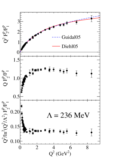
Figure 13: (color online) Data for the ratio $F_{2}^{p}/F_{1}^{p}$ from selected polarization experiments including Refs. Crawford et al. (2007); Punjabi et al. (2005a); Puckett et al. (2010); Jones et al. (2006); Maclachlan et al. (2006); Milbrath et al. (1998); Ron et al. (2011); Zhan et al. (2011) and the final GEp-II data from Table 4 of this work. From top to bottom: $Q^{2}F_{2}^{p}/F_{1}^{p}$, $QF_{2}^{p}/F_{1}^{p}$ and $Q^{2}/\ln^{2}\left(Q^{2}/\Lambda^{2}\right)F_{2}^{p}/F_{1}^{p}$, where $\Lambda=236$ MeV was fitted to the data for $Q^{2}\geq 1$ GeV². The curves in the top panel are GPD model fits from Guidal et al. (2005) (Guidal05) and Diehl et al. (2005) (Diehl05).

Figure 13 shows the experimental data for $F_{2}^{p}/F_{1}^{p}$ plotted as $Q^{2}F_{2}^{p}/F_{1}^{p}$, $QF_{2}^{p}/F_{1}^{p}$ and $Q^{2}/\ln^{2}\left(Q^{2}/\Lambda^{2}\right)F_{2}^{p}/F_{1}^{p}$. Clearly, the leading-twist, leading-order pQCD scaling behavior is not respected by the data in the presently accessible $Q^{2}$ region, although the slope of $Q^{2}F_{2}^{p}/F_{1}^{p}$ does appear to be trending toward a flat behavior at the highest-$Q^{2}$ values measured so far. The scaling of $QF_{2}/F_{1}$ predicted by Ralston and Jain (2004) is approximately satisfied up to 8.5 GeV², although there is a hint that $F_{2}$ may start to fall faster than $F_{1}/Q$ for higher $Q$. The logarithmic scaling of Belitsky et al. (2003) is satisfied for $Q^{2}\gtrsim 1$ GeV² at a value of the cutoff parameter $\Lambda=236$ MeV ($\hbar c/\Lambda=0.835$ fm) determined by fitting the data for $Q^{2}\geq 1$ GeV².

While the “precocious” scaling of $F_{2}^{p}/F_{1}^{p}$ is interesting, it is probably largely accidental, perhaps a consequence of delicate cancellations of higher-order effects in the ratio Belitsky et al. (2003). The scaling of $F_{2}^{p}/F_{1}^{p}$ is a necessary but insufficient condition for the onset of the perturbative regime. pQCD-based form factor predictions based on light-cone sum rules Braun et al. (2006); Passek-Kumericki and Peters (2008) have yet to reach the level of accuracy achieved by the phenomenological models discussed below in describing all four nucleon form factors. In the GPD model fits shown in Figure 13, the ’Feynman’ mechanism corresponding to the overlap of soft wavefunctions dominates the form factor behavior. The neutron data for $F_{2}^{n}/F_{1}^{n}$ do not scale in the currently measured $Q^{2}$ region up to 3.4 GeV² for values of $\Lambda$ similar to that which describes the proton data Riordan et al. (2010). Moreover, combining the proton and neutron data to separate the up and down-quark contributions to the nucleon form factors Cates et al. (2011) reveals that the ratios $F_{2}^{u}/F_{1}^{u}$ and $F_{2}^{d}/F_{1}^{d}$ become approximately constant above 1 GeV², at odds with the asymptotic pQCD picture, while the ratios $F_{1}^{d}/F_{1}^{u}$ and $F_{2}^{d}/F_{2}^{u}$ decrease at high $Q^{2}$, a behavior that can be explained in terms of diquark degrees of freedom Cloët et al. (2009). Based on these and other considerations, it is generally believed that the nucleon form factors are dominated by non-perturbative physics in the 1-10 GeV² region addressed by present experiments.

IV.2.2 Generalized Parton Distributions

The generalized parton distributions (GPDs) are universal non-perturbative matrix elements involved in the QCD factorization of hard exclusive processes such as deeply virtual Compton scattering (DVCS) Radyushkin (1996); Ji (1997a, b); Goeke et al. (2001). The GPDs are functions of the longitudinal momentum fraction $x$, the momentum fraction asymmetry or “skewness” $\xi$ and the squared momentum transfer to the nucleon $t$ (not to be confused with the photon virtuality $Q^{2}$). GPDs play a crucial role in the synthesis of seemingly disparate nucleon structure information obtained from inclusive and exclusive reactions. The Dirac and Pauli form factors $F_{1}$ and $F_{2}$ equal the first $x$ moments of the vector ($H(x,t)$) and tensor ($E(x,t)$) GPDs, respectively. In the forward ($t\rightarrow 0$) limit, $H(x,t=0)$ is the valence quark density. Precise measurements of the Pauli form factor $F_{2}$ at large $Q^{2}$ constrain the behavior of $E(x,t)$, yielding new information on nucleon structure that is inaccessible in inclusive deep inelastic scattering (DIS). With increasing $Q^{2}$, the strength in the GPD integrals corresponding to the form factors is increasingly concentrated in the high-$x$ region. Therefore, the $x\rightarrow 1$ behavior of $H(x,t)$ and $E(x,t)$ can be constrained by fitting the high-$Q^{2}$ nucleon form factors.

While systematic studies of the observables of DVCS and other hard exclusive reactions promise an eventual direct extraction of GPDs from global analysis (for recent examples, see Guidal (2008); Kumericki and Mueller (2010); Goldstein et al. (2011); Moutarde (2009); Kumericki et al. (2011)), the experimental mapping of these observables is still at an early stage. Meanwhile, constraints from the elastic form factors and the forward parton distributions measured in DIS have been explored using physically motivated GPD parametrizations based on Regge phenomenology Diehl et al. (2005); Guidal et al. (2005). In both models, the high-$x$ behavior of $E$ was determined by the high $Q^{2}$ behavior of $F_{2}^{p}$ measured by the GEp-I and GEp-II experiments, enabling an evaluation of Ji’s sum rule Ji (1997a, b) for the total angular momentum carried by the up ($J^{u}$) and down ($J^{d}$) quarks in the nucleon. The calculations of Guidal et al. (2005) found $2J^{d}=-0.06$ and $2J^{u}=+0.58$, in qualitative agreement with lattice QCD calculations available at the time Göckeler et al. (2004), as well as more recent calculations Hägler et al. (2008); Alexandrou et al. (2011). The predictions of the GPD models of Guidal et al. (2005) and Diehl et al. (2005) are compared to the data for $Q^{2}F_{2}^{p}/F_{1}^{p}$ in Figure 13.

The two-dimensional Fourier transform of the $t$-dependence of the GPDs at $\xi=0$ yields a three-dimensional impact parameter representation $\rho(x,\mathbf{b}_{\perp})$ in two transverse spatial dimensions and one longitudinal momentum dimension Burkardt (2003). By forming the charge-squared weighted sum over quark flavors and integrating over all $x$, Miller Miller (2007) derived the model-independent infinite momentum frame transverse charge density $\rho_{ch}(b)$ as the two-dimensional Fourier transform of the Dirac form factor $F_{1}$. The Pauli form factor $F_{2}$ can also be related to the transverse anomalous magnetic moment density $\rho_{m}(\mathbf{b})$ Miller (2010). Miller et al. Venkat et al. (2011) performed the first analysis of the uncertainties in the transverse charge and magnetization densities of the proton due to the uncertainties and incomplete $Q^{2}$ coverage of the form factor data. Measurements of $G_{E}^{p}$ at yet higher $Q^{2}$ are needed to reduce the uncertainty in $\rho_{m}(b)$ at small $b$.

Since an exact solution to QCD in the non-perturbative regime is not yet possible, predicting nucleon form factors in the domain of strong coupling and confinement is rather difficult. Consequently, many phenomenological models have aimed to unravel the complicated internal structure of the nucleon in this domain. The following discussion provides an overview of a wide range of models.

IV.2.3 Vector Meson Dominance

The global features of the nucleon form factors were explained by early models based on vector meson dominance (VMD) Iachello et al. (1973). VMD models are a special case of dispersion relation analyses, which provide a model-independent, non-perturbative framework to interpret the electromagnetic structure of the nucleon in both the space-like and time-like regions. Early VMD model calculations included the $\rho$ and its excited states for the isovector form factors, and the $\omega$ and $\phi$ for the isoscalar form factors. The number of mesons included and the coupling constants and masses can be varied to fit the data. In practice, many parameters are fixed or strongly constrained by experimental data, including but not limited to nucleon FF data, reducing the number of free parameters and increasing the predictive power of the approach. More recent calculations have used the pQCD scaling relations to constrain the large $Q^{2}$ behavior of the fits. An example is Lomon’s fit Lomon (2002), which uses $\rho(770)$, $\omega(782)$, $\phi(1020)$, $\rho^{\prime}(1450)$ and $\omega^{\prime}(1420)$ mesons and has a total of 12 variable parameters Lomon (2002, 2006). Bijker and Iachello Bijker and Iachello (2004) updated the 1973 model of Iachello, Jackson and Landé Iachello et al. (1973), performing a new fit including the $\rho(770)$, $\omega(782)$, and $\phi(1020)$ mesons, and a phenomenological “direct coupling” term attributed to an intrinsic three-quark structure of $rms$ radius $\sim 0.34$ fm.

Despite the relatively good fits obtained by VMD models, the approach is at odds with general constraints from unitarity. This difficulty can be overcome using dispersion relations. Höhler’s dispersion relation analysis Höhler et al. (1976) was extended in the mid-nineties by Mergell, Meissner, and Drechsel Mergell et al. (1996) to include nucleon form factor data in the time-like region Hammer et al. (1996). The analysis of Mergell et al. (1996) has been further improved by Belushkin et al. Belushkin et al. (2007). In addition to the $2\pi$ continuum present in the isovector spectral functions, the $\rho\pi$ and $K\bar{K}$ continua were included in the isoscalar spectral functions. In Belushkin et al. (2007), the $2\pi$ continuum was reevaluated using the latest experimental data for the pion form factors in the time-like region. A simultaneous fit to the world data for all four form factors in both the space-like and time-like regions was performed. The results are in very good agreement with the data available at the time. Dubnicka et al. developed a unitary and analytic ten-resonance model including the $2\pi$ continuum Dubnicka et al. (2003); Adamuscin et al. (2005), which fits all nucleon form factors in both the space-like and time-like regions.

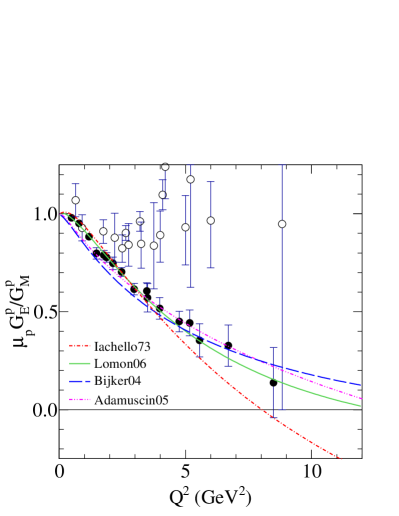
Figure 14: (color online) Comparison of selected VMD model predictions from Iachello et al. (1973) (Iachello73), Lomon (2006) (Lomon06), Bijker and Iachello (2004) (Bijker04), and Adamuscin et al. (2005) (Adamuscin05) to selected $\mu_{p}G_{E}^{p}/G_{M}^{p}$ data. Data are from cross section Andivahis et al. (1994); Christy et al. (2004); Qattan et al. (2005) (empty circles) and polarization Punjabi et al. (2005a); Gayou et al. (2002); Puckett et al. (2010) (filled circles) measurements, where the results of Gayou et al. (2002) are replaced by the results of the present work. See text for details.

Figure 14 compares the predictions of selected VMD-based models to the experimental data for $\mu_{p}G_{E}^{p}/G_{M}^{p}$. Of the models shown, the latest version of Lomon’s fit Lomon (2006) with twelve adjustable parameters achieves the best overall agreement with the data for all four form factors at spacelike $Q^{2}$, emphasizing a smooth evolution from VMD behavior at low $Q^{2}$ to pQCD scaling at asymptotically high $Q^{2}$. Apart from fitting to a more complete data set, the main added feature of the model of Bijker and Iachello Bijker and Iachello (2004) relative to the 1973 model of Iachello, Jackson and Landé is the inclusion of a “direct” coupling term in the isoscalar Pauli form factor which improves the large-$Q^{2}$ behavior of $G_{E}^{p}$ and $G_{E}^{n}$. This model achieves a rather good fit to all four FFs using just six adjustable parameters (compared to five in the 1973 model).

IV.2.4 Lattice QCD

Lattice QCD calculations provide ab initio evaluations of static and dynamic hadron properties, including the nucleon electromagnetic form factors, from numerical solutions of QCD on a finite-volume lattice of discrete space-time points. At present, the lattice calculations are done using unphysically large quark masses which are given in terms of the pion mass, $m_{\pi}$. Moreover, most recent calculations focus on the isovector form factors, for which the contributions from disconnected diagrams are reduced. Calculations are performed for various $m_{\pi}$ values and lattice spacings $a$ and then extrapolated to the physical pion mass and the continuum limit $a\rightarrow 0$. Recently the QCDSF/UKQCD Collaboration has performed calculations Collins et al. (2011) at $m_{\pi}=180$ MeV with different lattice spacings and volume sizes, but the upper $Q^{2}$ range is limited to 3 GeV². Lattice QCD form factor calculations in the $Q^{2}$ region measured by the GEp-II and GEp-III experiments are difficult due to large statistical and systematic errors. Calculations by Lin et al. employ a novel technique to extend the reliable $Q^{2}$ range of the calculations to $Q^{2}=6$ GeV² at $m_{\pi}>450$ MeV for quenched and dynamical ensembles Lin et al. (2010). Nonetheless, calculations at such high $Q^{2}$ must ultimately be performed with a finer lattice spacing to reduce the systematic error.

IV.2.5 Constituent Quark Models

In the constituent quark model (CQM), the nucleon consists of three constituent quarks, which can be thought of as valence quarks that become much heavier than the elementary quarks appearing in the QCD Lagrangian when dressed by gluons and quark-antiquark pairs. The dressing effects are absorbed into the masses of these quasiparticle effective degrees of freedom. The early non-relativistic constituent quark model achieved considerable success in describing the spectrum of baryons and mesons with correct masses Isgur and Karl (1978). In order to describe dynamical quantities such as form factors in terms of constituent quarks, a relativistic description (rCQM) is mandatory because the $Q^{2}$ values involved in modern experiments have reached as high as ten times the nucleon mass squared and $\sim 10^{6}$ times the “bare” quark mass squared.

Frank et al. Frank et al. (1996) calculated $G_{E}^{p}$ and $G_{M}^{p}$ in the light-front CQM using the light-front nucleon wave function of Schlumpf Schlumpf (1993), and predicted that $G_{E}^{p}$ might change sign near 5.6 GeV², a behavior inconsistent with current data, though qualitatively correct. In this model, constructing a Poincaré-invariant nucleon wavefunction that is also an eigenstate of spin leads to the substantial violation of hadron helicity conservation Miller and Frank (2002) responsible for the observed scaling of $QF_{2}/F_{1}$ in the $Q^{2}$ range of present experiments. This feature is a consequence of the unitary Melosh rotation Melosh (1974) which mixes quark spin states in the process of boosting the nucleon spin-flavor wavefunction from the rest frame to the light front. Miller extended this model to include pion-cloud effects Miller (2002), important to the understanding of the low-$Q^{2}$ behavior generally and $G_{E}^{n}$ in particular.

Gross et al. Gross and Agbakpe (2006); Gross et al. (2008) modeled the nucleon as a bound state of three dressed valence constituent quarks in the covariant spectator formalism, in which the virtual photon is absorbed by an off-shell constituent quark, and the two spectator quarks always propagate as an on-shell diquark. In this model, the constituent quarks have internal structure described by form factors which become pointlike at large $Q^{2}$ as required by pQCD and exhibit VMD-like behavior at low $Q^{2}$. The model nucleon wavefunction of Gross et al. (2008) obeys the Dirac equation, includes only s-wave components, and its spin-isospin structure reduces to that of the SU(2) $\times$ SU(2) quark model in the non-relativistic limit.

Cardarelli et al. Cardarelli and Simula (2000) calculated the ratio using light-front dynamics and investigated the effects of SU(6) symmetry breaking. As in Frank et al. (1996), they showed that the decrease of $R$ with increasing $Q^{2}$ is caused by the relativistic effect of the Melosh rotations of the constituent quark spins. De Sanctis et al. calculated the nucleon form factors in the relativistic hypercentral constituent quark model (hCQM) Sanctis et al. (2007). A good fit to all the nucleon form factors was obtained using a linear combination of monopole and dipole constituent quark form factors. The calculation was recently extended to $Q^{2}=12$ GeV² Santopinto et al. (2010). The same group also performed calculations within the relativistic interacting quark-diquark model De Sanctis et al. (2011), which does not achieve the same level of agreement with the data as the hCQM.

De Melo et al. de Melo et al. (2009) examined the non-valence components of the nucleon state in light-front dynamics, achieving a good description of all spacelike and timelike nucleon FF data with the inclusion of the Z-diagram involving $q\bar{q}$ pair creation in addition to the triangle (valence) diagram. The chiral constituent quark model based on Goldstone-boson-exchange dynamics was used by Boffi et al. Boffi et al. (2002) to describe the elastic electromagnetic and weak form factors in a covariant framework using the point-form approach to relativistic quantum mechanics.

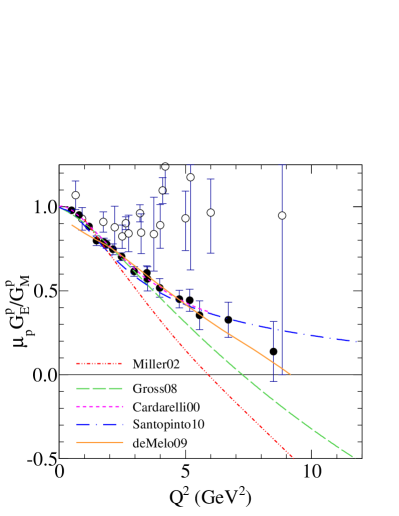
Figure 15: (color online) Selected rCQM predictions from Miller (2002) (Miller02), Gross et al. (2008) (Gross08), Cardarelli and Simula (2000) (Cardarelli00), Santopinto et al. (2010) (Santopinto10) and de Melo et al. (2009) (deMelo09) for $R=\mu_{p}G_{E}^{p}/G_{M}^{p}$, compared to selected data from cross section Andivahis et al. (1994); Christy et al. (2004); Qattan et al. (2005) (empty circles) and polarization Punjabi et al. (2005a); Gayou et al. (2002); Puckett et al. (2010) (filled circles) experiments, where the results of Gayou et al. (2002) are replaced by the results of the present work. See text for details.

Figure 15 compares the predictions of selected rCQM calculations to selected data for $R$. Of the calculations shown, those in which the constituent quarks have internal structure represented by CQ form factors (Cardarelli and Simula (2000); Gross et al. (2008); Santopinto et al. (2010)) and/or significant VMD-related contributions to the photon-nucleon vertex (de Melo et al. (2009)) describe the data better than those in which the constituent quarks are pointlike (Miller (2002)) and have only direct coupling to the photon. Although this may be related to the greater number of adjustable parameters in models with CQFFs, it is apparently physically meaningful that most of the models require structure of the constituent quarks and/or significant nonvalence ($q\bar{q}$ pair creation) contributions to achieve a good description of the data.

IV.2.6 Dyson-Schwinger Equations

A different theoretical approach to the prediction of nucleon form factors is based on QCD’s Dyson-Schwinger equations (DSEs). The DSEs are an infinite tower of coupled integral equations for QCD’s Green functions that provide access to emergent phenomena of non-perturbative QCD, such as dynamical chiral symmetry breaking and confinement Roberts and Williams (1994). The DSEs admit a symmetry-preserving truncation scheme that enables a unified description of meson and baryon properties. The approach has already achieved considerable success in the pseudoscalar meson sector Roberts (2008). The prediction of nucleon form factors in the DSE approach involves the solution of a Poincaré-covariant Faddeev equation. In the calculations of Cloët et al. (2009), dressed quarks form the elementary degrees of freedom and correlations between them are expressed via scalar and axial vector diquarks. The only variable parameters in this approach are the diquark masses, fixed to reproduce the nucleon and $\Delta$ masses, and a diquark charge radius $r_{1}^{+}$ embodying the electromagnetic structure of the diquark correlations. A different approach to DSE-based form factor calculations effects binding of the nucleon through a single dressed gluon exchange between any two quarks Eichmann (2011) without explicit diquark degrees of freedom. In this calculation, the only parameters are a scale fixed to reproduce the pion decay constant and a dimensionless width parameter $\eta$ describing the infrared behavior of the effective coupling strength of the quark-quark interaction.

The predictions of several DSE-based calculations for the proton Sachs form factor ratio $R=\mu_{p}G_{E}^{p}/G_{M}^{p}$ are shown in Figure 16. The quark-diquark model calculation Cloët et al. (2009) underpredicts the data at low $Q^{2}$ but agrees reasonably well at higher $Q^{2}$. The disagreement at low $Q^{2}$ is attributed to the omission of meson cloud effects. The addition of dynamically generated, momentum-dependent dressed-quark anomalous magnetic moments Chang et al. (2011) that become large at infrared momenta improves the description of $R$ at low $Q^{2}$. The three-quark model calculation Eichmann (2011) agrees with the data at low $Q^{2}$, but underpredicts the data at higher $Q^{2}$, becoming numerically unreliable for $Q^{2}\gtrsim 7$ GeV².

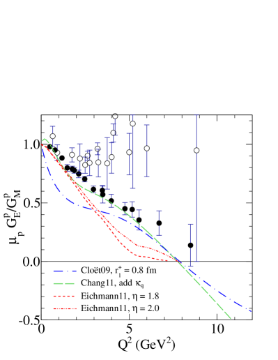
Figure 16: (color online) Predictions of DSE-based calculations for $R=\mu_{p}G_{E}^{p}/G_{M}^{p}$ compared to experimental data from cross section Andivahis et al. (1994); Christy et al. (2004); Qattan et al. (2005) (empty circles) and polarization Punjabi et al. (2005a); Gayou et al. (2002); Puckett et al. (2010) (filled circles) experiments, where the results of Gayou et al. (2002) are replaced by those of the present work. The results of Cloët et al. (2009) (Cloët09) are shown for a particular choice of the diquark charge radius. The curve from Chang et al. (2011) (Chang11) is that of Cloët et al. (2009) with the addition of dressed quark anomalous magnetic moments. The results of Eichmann (2011) (Eichmann11) are shown for two values of $\eta$, showing the weak sensitivity of the form factor results to this parameter.

The deficiencies of the DSE approach, including the approximation schemes required to make the calculations analytically tractable and the omission of meson-cloud effects, are evident in the disagreement between the predicted form factors and the experimental data, which is more severe than in the various models described above, which have more adjustable parameters. The advantage of the approach is that it provides a systematically improvable framework for the ab initio evaluation of hadron properties in continuum non-perturbative QCD, that is complementary to discretized lattice simulations. As fundamental measurable properties of nucleon structure, the electromagnetic form factors are essential to the feedback between theory and experiment required to make further progress in this direction.

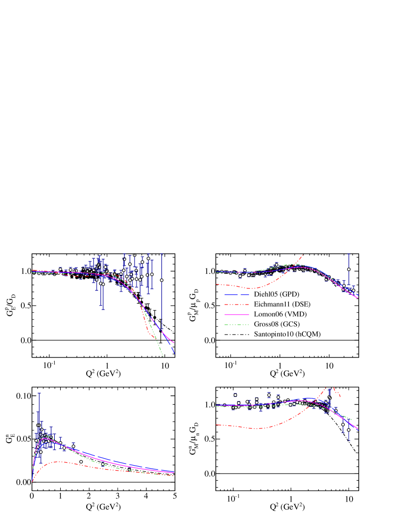
Figure 17: (color online) Comparison of selected theoretical predictions to data for all four nucleon FFs at space-like $Q^{2}$. Theory curves are Diehl et al. (2005) (Diehl05), Eichmann (2011) (Eichmann11), Lomon (2006) (Lomon06), Gross et al. (2008) (Gross08) and Santopinto et al. (2010) (Santopinto10). $G_{E}^{p}$ data are from Andivahis et al. (1994); Borkowski et al. (1975); Christy et al. (2004); Janssens et al. (1966); Price et al. (1971); Qattan et al. (2005); Simon et al. (1980); Walker et al. (1994); Berger et al. (1971) (cross section data, empty circles) and Crawford et al. (2007); Punjabi et al. (2005a); Gayou et al. (2002); Puckett et al. (2010); Jones et al. (2006); Maclachlan et al. (2006); Milbrath et al. (1998); Ron et al. (2007); Zhan et al. (2011) (polarization data, filled circles), where the results of Gayou et al. (2002) have been replaced by the results of the present work (Table 4). $G_{M}^{p}$ data are from Bartel et al. (1973); Berger et al. (1971); Andivahis et al. (1994); Borkowski et al. (1975); Christy et al. (2004); Kirk et al. (1973); Janssens et al. (1966); Price et al. (1971); Qattan et al. (2005); Sill et al. (1993); Walker et al. (1994). $G_{E}^{n}$ data are from Bermuth et al. (2003); Eden et al. (1994); Geis et al. (2008); Glazier et al. (2005); Herberg et al. (1999); Meyerhoff et al. (1994); Ostrick et al. (1999); Passchier et al. (1999); Plaster et al. (2006); Riordan et al. (2010); Rohe et al. (1999); Warren et al. (2004); Zhu et al. (2001). $G_{M}^{n}$ data are from Anklin et al. (1994, 1998); Lachniet et al. (2009); Bruins et al. (1995); Gao et al. (1994); Lab E95-001 Collaboration (2007); Kubon et al. (2002); Lung et al. (1993); Markowitz et al. (1993); Rock et al. (1982); Xu et al. (2000, 2003). $G_{D}=\left(1+Q^{2}/\Lambda^{2}\right)^{-2}$, with $\Lambda^{2}=0.71$ GeV², is the standard dipole form factor.

IV.2.7 AdS/QCD

In the past decade, theoretical activity has flourished in modeling QCD from the conjecture of the anti-de Sitter space/conformal field theory (AdS/CFT) correspondence Maldacena (1998); Witten (1998); Gubser et al. (1998), a mapping between weakly coupled gravitational theories in curved five-dimensional space-time and strongly coupled gauge theories in flat four-dimensional space-time. Since QCD is not a conformal field theory, the symmetry of the anti-de Sitter space is broken by applying a boundary condition. Brodsky and de Teramond Brodsky and de Teramond (2008) have calculated $F_{1}$ for the proton and neutron and emphasized the agreement of the predicted $Q^{2}F_{1}$ dependence with the data. Abidin and Carlson Abidin and Carlson (2009) have calculated both proton and neutron $F_{1}$ and $F_{2}$ along with the tensor form factors using both hard and soft wall boundary conditions. This model predicts the same asymptotic $Q^{2}$ dependence as the dimensional scaling of pQCD, but does not reproduce the detailed features of the data in the presently measured $Q^{2}$ region.

IV.2.8 World nucleon form factor data compared to theory

Figure 17 summarizes the theoretical interpretation of the nucleon electromagnetic form factors, with representative examples from each of the classes of models discussed compared to the world data for all four nucleon electromagnetic form factors. Published results for $R=\mu_{p}G_{E}^{p}/G_{M}^{p}$ were converted to $G_{E}^{p}$ values using the global fit of $G_{E}^{p}$ and $G_{M}^{p}$ from Puckett (2010), updated to use the $R$ values of the present work, a change that does not noticeably affect $G_{M}^{p}$. Except at very low $Q^{2}$, the contribution of the uncertainty in $G_{M}^{p}$ to the resulting uncertainty in $G_{E}^{p}$ is negligible. At this juncture, it is worth recalling that the $G_{E}^{p}$ results extracted from cross section data are believed to be unreliable at high $Q^{2}$ due to incompletely understood TPEX corrections, which have not been applied to the data shown in Figures 14-17. Except for the DSE calculation of Eichmann (2011), all of the models shown describe existing data very well, which is to be expected given that the parameters of the models are fitted to reproduce the data. However, their predictions tend to diverge when extrapolated outside the $Q^{2}$ range of the data. That the DSE-based calculation of Eichmann (2011) fails to describe the data as well as the other calculations is not surprising, since it represents a more fundamental ab initio approach with virtually no adjustable parameters, but requires approximations that are not yet well-controlled. Significant progress in the quality of the predictions is nonetheless evident, as the data expose the weaknesses of different approximation schemes. Since the hard scattering mechanism leading to the asymptotic pQCD scaling relations is not expected to dominate the form factor behavior at presently accessible $Q^{2}$ values, phenomenological models and the ambitious ongoing efforts in lattice QCD and DSE calculations are of paramount importance to understanding the internal structure and dynamics of the nucleon. Planned measurements at higher $Q^{2}$ following the 12 GeV upgrade of JLab promise to be of continuing interest and relevance owing to their power to discriminate among the various models and to guide the improvement of the more fundamental calculational approaches.

V Conclusion

This work has presented an expanded description and an improved final data analysis of the GEp-II experiment, originally published in Gayou et al. (2002), which measured the proton electromagnetic form factor ratio for $3.5\mbox{ GeV}^{2}\leq Q^{2}\leq 5.6$ GeV² in Jefferson Lab’s Hall A using the polarization transfer method. The improved data analysis finds a systematic increase in the results for $R=\mu_{p}G_{E}^{p}/G_{M}^{p}$ that improves the agreement between the GEp-II and GEp-III Puckett et al. (2010) data. This increase mainly reflects the underestimated impact of the $\pi^{0}$ production background in the original analysis of GEp-II. Section II presented the details of the experimental apparatus and described the differences between the GEp-II and GEp-III experiments. Section III presented the full details of the data analysis, including the selection of elastic events in section III.1, the extraction of polarization observables in section III.2, and the treatment of the background in section III.3. The analysis of systematic uncertainties was presented in section III.4. In section IV.1, the features of the data and the sources of the increase in the results relative to the original analysis were discussed at length. An overview of recent progress in the theoretical understanding of nucleon form factors was given in section IV.2. In conclusion, this work represents the final results of the GEp-II experiment. The revised data presented here and the results of the GEp-III experiment Puckett et al. (2010) have considerably improved the experimental knowledge of $G_{E}^{p}$ at large $Q^{2}$.