Momentum distribution and ordering in mixtures of ultracold light and heavy fermionic atoms

Abstract

The momentum distribution is one of the most important quantities which provides information about interactions in many-body systems. At the same time it is a quantity that can easily be accessed in experiments on ultracold atoms. In this paper, we consider mixtures of light and heavy fermionic atoms in an optical lattice described effectively by the Falicov-Kimball model. Using a Monte Carlo method, we study how different ordered density-wave phases can be detected by measurement of the momentum distribution of the light atoms. We also demonstrate that ordered phases can be seen in Bragg scattering experiments. Our results indicate that the main factor that determines the momentum distribution of the light atoms is the trap confinement. On the other hand, the pattern formed by the heavy atoms seen in the Bragg scattering experiments is very sensitive to the temperature and possibly can be used in low-temperature thermometry.

I Introduction

It is well known that the equilibrium momentum distribution of free noninteracting fermions is described by the Fermi-Dirac distribution function. When interactions are turned on, the momentum distribution is changed due to these interactions. Similarly, if the noninteracting gas is confined in a harmonic trap, the distribution can also be calculated explicitly rigol , however in the limit of a large number of fermions it is convenient to use the semiclassical Thomas–Fermi approximation butt or other semiclassical approaches march . The situation becomes much more complicated if the interaction between fermions cannot be neglected. Then, numerical methods usually need to be applied, especially when the system is in a trap. On the other hand, the momentum distribution function is a quantity that can be directly accessed in experiments with ultracold atomic gases and therefore it is of a particular importance in trying to make contact between theory and experiment.

We examine the problem of a mixture of different mass fermionic atoms on an optical lattice at low temperature. Since most stable heavy isotopes of alkalies are bosonic, we envision mixtures of Li⁶ with K⁴⁰, or light Li⁶ or K⁴⁰ mixed with heavy fermionic isotopes of Sr or Yb (it turns out that if the heavy particle is a boson with strong enough intraspecies repulsion, and one is at a low enough temperature, then the statistics of the heavy particle does not enter into our model, as it appears effectively like a hardcore object). We have already performed numerical calculations on this system and shown that one can see interesting phenomena similar to viscous fingering as one tunes the trap curvature for the light species and moves from a phase separated state with the heavies on the outside to one with the heavies on the inside PRL . Interesting ordered density-wave patterns appear at low temperature in these mixtures. The question is, how do we detect the presence of such order with current experimentally available techniques? In situations where in situ imaging with single-site precision is available Greiner , one would simply look for the ordered phases directly, just as they appear in the Monte Carlo snapshots of a particular configuration of the atoms. But can one see effects of the density-wave ordering in a time-of-flight image, or via direct Bragg scattering of light off of the density-wave pattern? We answer these questions here.

In Section II, we introduce the model and the techniques used to solve for the equilibrium properties of the mixtures of fermions in a harmonic trap. In Section III, we present our numerical results. Conclusions follow in Section IV.

II The model and method

A mixture of light and heavy fermionic atoms in a harmonic trap (each in one and only one hyperfine atomic state and hence acting like a spinless fermion), under the assumption that the quantum-mechanical effects of the hopping of the heavy atoms can be neglected, is described by the Falicov–Kimball Hamiltonian FK ; Ziegler

$${\cal H}= - J\sum_{\langle i,j\rangle}\left(c^{\dagger}_{i}c_{j}+c^{\dagger}_{j}c_{i}\right)+\sum_{i}\left(V_{i}-\mu\right)c^{\dagger}_{i}c_{i}$$ (1)

$$+ \sum_{i}\left(V^{h}_{i}-\mu^{h}\right)w_{i}+U\sum_{i}c^{\dagger}_{i}c_{j}w_{i},$$

where $c^{\dagger}_{i}$ is an operator that creates a light fermionic atom at site $i$ and $U$ is the on–site interspecies interaction potential. The symbol $V_{i}$ is the light particle trap potential, and $\mu$ is its chemical potential. $V_{i}^{h}$ is the trap for the heavy atoms and $\mu^{h}$ is its respective chemical potential. The symbol $w_{i}=0$ or 1 is the number operator of the heavy particles, which can be treated as a classical variable since the heavy particles do not hop. The same Hamiltonian can also describe Fermi-Bose mixtures, provided the bosonic atoms are the heavy (localized) ones and a strong repulsion between them prevents them from occupying one site by two bosons (hard core bosons). This model can easily be extended to describe a system with soft-core bosons. In such a case $w_{i}=0,1,2,\ldots$ and an additional term describing the boson-boson on-site interaction

$${\cal H}_{\rm B-B}=\frac{1}{2}U_{\rm B-B}\sum_{i}w_{i}(w_{i}-1)$$ (2)

has to be added to the Hamiltonian in Eq. (1) vollhardt ; iskin . The trap potentials for the light ($V_{i}$) and heavy ($V^{h}_{i}$) atoms are given by

$$V_{i}=\frac{J}{R^{2}}\left(x_{i}^{2}+y_{i}^{2}\right),\ \ \ V^{h}_{i}=\frac{J}{\left(R^{h}\right)^{2}}\left(x_{i}^{2}+y_{i}^{2}\right)$$ (3)

where $(x_{i},y_{i})$ is the position of site $i$ ($a$ is the lattice constant). The steepness of the potential confining the light atoms varies from $R=30a$ to $R=12.9a$, whereas it is fixed for the heavy atoms with $R^{h}=30a$. The chemical potentials $\mu$ and $\mu^{h}$ have been introduced in order to control the number of the light and heavy atoms, respectively.

The model is solved by means of a variation of the Monte Carlo (MC) method. The method is based on the classical Metropolis algorithm modified in such a way that systems with both quantum and classical degrees of freedom can be simulated MC . In each MC step, a new configuration of the heavy atoms is generated. Then, the Hamiltonian in Eq. (1) is numerically diagonalized to yield all the eigenenergies and eigenstates of the light atoms for the trial configuration of the heavy atoms. The new configuration of the heavy atoms is accepted according to the same rules as in the Metropolis algorithm, but with the free energy of the light atoms used for comparing energies instead of the internal energy. The results are then averaged over all the configurations generated during the entire MC run. Real-space configurations of the atoms for different model parameters (interaction, shape of the trapping potential) at different temperatures have been studied in Ref. PRL, . In the present paper we use a similar method to investigate the momentum distribution and Bragg scattering spectra. Since diagonalization of the Hamiltonian in Eq. (1) for a given configuration of the heavy atoms gives all the eigenstates of the light atoms, it allows one to also calculate the momentum distribution of the light atoms. Under the assumption that the optical lattice potential is deep enough that we can restrict to a single-band model, then the field operator of these atoms $\Psi({\bm{r}})$ (expanded in terms of the Bloch wavefunctions for the lowest band) is given by

$$\Psi({\bm{r}})={\sum_{\bm{k}}}c_{\bm{k}}\Psi_{\bm{k}}({\bm{r}}),$$ (4)

where $c_{\bm{k}}=1/N\sum_{i}c_{i}\exp\left(-i{\bm{k}}\cdot{\bm{R}}_{i}\right)$ and $\Psi_{\bm{k}}({\bm{r}})$ is the Bloch wavefunction. Expanding the Bloch wavefunction in terms of the Wannier wavefunctions of the lowest band $w({\bm{r}}-{\bm{R}}_{i})$ which are localized about lattice site ${\bm{R}}_{i}$ yields $\Psi_{\bm{k}}({\bm{r}})=1/\sqrt{N}\sum_{i}w({\bm{r}}-{\bm{R}}_{i})\exp\left(i{\bm{k}}\cdot{\bm{R}}_{i}\right)$. The summation runs over the first Brilliouin zone. Then, the free space momentum distribution can be calculated as wang

$$n({\bm{k}})=|w({\bm{k}})|^{2}c^{\dagger}_{\bm{k}}c_{\bm{k}},$$ (5)

where $w({\bm{k}})$ is the Fourier transform of the Wannier function. Hence the momentum distribution can be approximated by

$$n({\bf k})=\frac{\left|w({\bm{k}})\right|^{2}}{N}\sum_{i,j}\langle c^{\dagger}_{i}c_{j}\rangle e^{i{\bm{k}}\cdot\left({\bm{R}}_{i}-{\bm{R}}_{j}\right)}$$ (6)

in the single-band limit, with $N$ the number of lattice sites.

Here, the quantum mechanical expectation value $\langle\ldots\rangle$ is calculated for a given configuration of the heavy atoms and therefore $n({\bm{k}})$ has to be averaged over the configurations.

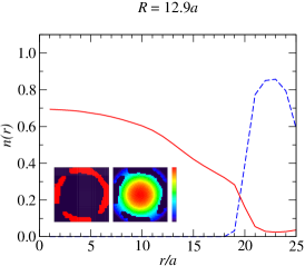
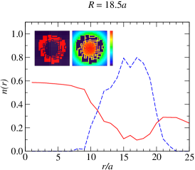
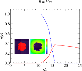
Figure 1: (Color online) Density profiles of the light (solid red line) and heavy (dashed blue line) atoms for $U=5J$ at a temperature $k_{\rm B}T=0.01J$. The curvature of the trap for the heavy atoms is given by $R^{h}=30a$, whereas for the light atoms it varies from $R=12.9a$ to $R=30a$. The insets show snapshots of real-space distributions of the heavy (left box) and light (right box) atoms.

We ignore dynamic interactions between heavy and light atoms due to scattering in the course of the expansion in the time-of-flight experiments. This is a reasonable approximation since the density of the clouds is very small once the trap and the optical lattice potentials are dropped. Since those potentials are dropped over a finite period of time, there can be some effects as the potentials are lowered, but these tend to be smaller in these systems because the repulsive interspecies interaction keeps the light and heavy particles away from each other in their initial distributions on the lattice prior to the time-of-flight experiment.

Since in our approximation the heavy atoms are localized, we are interested in the momentum distribution of only the light ones. The heavy atoms, however, may display some kind of density-wave ordering, which has been demonstrated in Ref. PRL, . In particular, for some regimes of parameters they form a checkerboard pattern where the heavy atoms occupy only, e.g., black squares. In another regime, superpositions of vertical and horizontal stripes or phase separation, with the heavy and light atoms occupying different regions of space have been observed. Of course, for any nonvanishing interaction between both species of atoms the distribution of the light atoms is up to some degree correlated with the distribution of the heavy ones. As a result, also the light atoms are ordered, but unless the interaction is strong enough, the magnitude of the density-wave order is much smaller. This follows from the fact that the light atoms, in contrast to the heavy ones, gain kinetic energy while delocalized.

The ordering of the heavy atoms can be analyzed by use of scattering of light (Bragg scattering, see e.g., Ref. Bragg, ). This kind of experiment is an equivalent to neutron or X-ray diffraction for the solid state. However, due to the difference of lattice constants between solid state crystals and optical lattices, the required wavelength corresponds to that of visible light. The observation of well-defined Bragg peaks has been used to confirm a crystalline structure formed by atoms in an optical lattice Bragg . Since this method allows one to determine the distance between atoms forming the crystalline structure, it can be applied in order to detect the checkerboard pattern as well. In the case of strong repulsive interaction between the light and heavy atoms, checkerboard squares of different color are occupied by different kinds of atoms and the problem is similar to the detection of antiferromagnetic (AF) order. It has recently been proposed to use Bragg diffraction of light to detect such an order Bragg_AFM in a Hubbard system. In the case of AF order, the spin–dependent scattering is achieved by using the probe light frequency near atomic resonance, where the interaction between light and atoms is neither purely diffractive nor purely absorptive. In a similar way the probe light can be tuned to be scattered in a different way by the light and heavy atoms. As a result, we can expect a $(\pi,\pi)$ peak in the case of a two-dimensional checkerboard pattern with the light scattered by the heavy atoms. Moreover, the intensity of this peak can give information about the fraction of the system occupied by ordered atoms. This method can also be used to detect other types of correlations. If the “labyrinthine” patterns obtained in Monte Carlo simulations PRL are superpositions or mixtures of horizontal and vertical stripes, the Bragg scattering in this case should reveal $(0,\pi)$ and $(\pi,0)$ peaks.

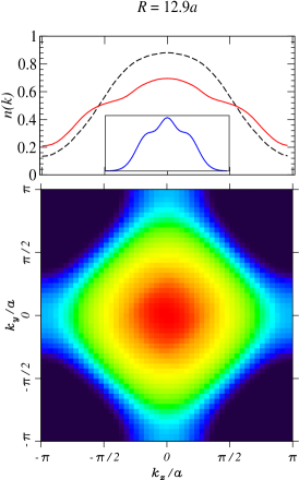
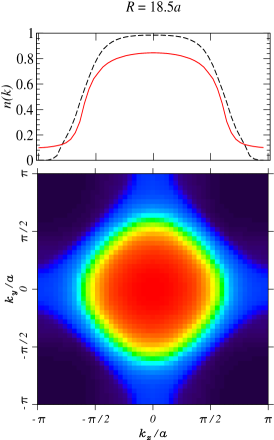
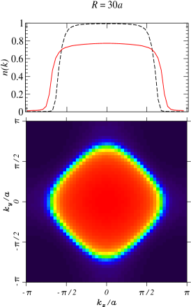
Figure 2: (Color online) Momentum distribution of the light atoms for the cases shown in Fig. 1. The upper row shows a comparison of cross sections along the $x$ axis for $U=5J$ (solid red line) and noninteracting case (dashed black line). The inset in the first plot shows the momentum distribution of the light atoms confined in a circular well with infinite walls (see text).

The Bragg spectra integrated over the frequency gives the static structure factor $S({\bm{k}})$, a key quantity that can be expressed as

$$S({\bm{k}})=\frac{1}{N}\sum_{i}w_{i}e^{i{\bm{k}}\cdot{\bm{R}}_{i}}.$$ (7)

In a practical realization we get a new configuration $\{w_{i}\}$ in each MC step and in each step $S({\bm{k}})$ is calculated. Then, $S({\bm{k}})$ is averaged over the entire MC run.

III Results

Simulations have been carried out on a $50\times 50$ square lattice with 625 heavy and 625 light atoms. In contrast to solid state simulations, there is no translational symmetry in the real system and therefore we use hard-wall boundary conditions at the edges. For steep harmonic trap potentials (and at low $T$) most of the atoms are in the center of the system, however, if the potentials are shallow the results may be affected by the finite size of the cluster. Fig. 1 illustrates the real-space distributions of the light and heavy atoms for different shapes of the trap for the light atoms [see Eq. (3) for the trap potential parametrization]. The trapping potential for the heavy atoms is kept at $R^{h}=30a$ for all simulations.

From Fig. 1 one can see that if the light atoms’ trap potential is sufficiently steep and the repulsion between the two species of atoms is relatively strong ($U=5J$), the heavy atoms are pushed out from the center of the trap. This is an intuitive result. However, when the trap potential for the light atoms becomes shallower they start to spread and occupy the periphery of the cluster even before the trap curvatures are set to be equal. For identical potentials, the heavy atoms are concentrated in the central part of the trap, surrounded by the light atoms. In such a configuration the light atoms can gain kinetic energy at the expense of the potential energy in the harmonic trap.

III.1 Momentum distribution of the light atoms

Fig. 2 shows the momentum distribution of the light atoms for the same parameters as in Fig. 1. Since the strong repulsion leads to phase separation, at least in the limiting cases, the light atoms are able to move freely within the region not occupied by the heavy atoms. Nevertheless, one can notice that there is no sign of the Fermi surface in the momentum distribution, which results from the inhomogeneity of the system. The upper row of panels presents a comparison of the crossections of the actual distribution with that of a noninteracting fermionic gas in a harmonic trap. The difference results from the interaction between the light and heavy atoms. Generally, for all the shapes of the trap potential, the maximal value of the momentum distribution function at ${\bf k}=0$ of the light atoms is reduced with respect to the noninteracting case. For a relatively steep trap potential for the light atoms, the interaction leads to an occurrence of additional features in the momentum distribution [see the red (solid) curve in the upper left panel of Fig. 2]. The occurrence of these additional inflection points results from a further confinement of the light atoms in an area surrounded by the heavy atoms, as can be seen in Fig. 3.

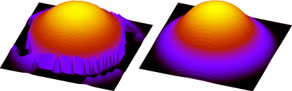
Figure 3: (Color online) Comparison of the real-space distribution of light atoms with (left graph, $U=5J$) and without (right graph) interaction with heavy atoms ($R=12.9a$).

In order to confirm the origin of these features, we calculated the momentum distribution of the light atoms in an infinite round well with a diameter equal to the inner diameter of the ring formed by the heavy atoms. In the resulting distribution, presented in the inset in Fig. 2, the additional peak in the center of the distribution is even more pronounced.

Independent of the strength of the interaction, the inhomogeneity destroys any signs of the Fermi edge in the momentum distribution. When the trap becomes shallower, behavior that looks like a Fermi edge appears, but this is due to the box boundary conditions at the edge of the lattice.

Even though there is no explicit signal in the momentum distribution function which shows the presence of different kinds of density wave ordering, the momentum distribution function does have a strong dependence on the appearance of phase separation, as can be seen in the different distribution functions in Fig.2. For example, it is known that in a homogeneous lattice, the momentum distribution function must decrease below the noninteracting value for small momentum and increase above the noninteracting value for large momentum ueltschi when the system phase separates at low temperature. This behavior is clearly seen in all of the data, and most likely is arising from different forms of quantum confinement effects associated with the phase separation. Unfortunately, it is not easy to disentangle this phase separation effect from the effect of the trap, which has a similar effect on the momentum distribution function, except in the case where the heavy particles surround the light ones and confine them with a sharp boundary. In that case, the phase separation effect causes a “dimple” in the momentum distribution function near ${\bm{k}}=0$.

If the interspecies repulsion is too weak to lead to phase separation, a checkerboard configuration may be formed. Fig. 4 shows examples of real-space configurations of the light atoms for $U=J$. It turns out that in this case the momentum distribution is hardly affected by the interaction. Fig. 5 presents a comparison of the momentum distribution at temperatures above and below the temperature, at which a checkerboard pattern is formed. When the temperature is lowered, the momentum distribution is enhanced for small ${\bm{k}}$, though the difference much smaller. Moreover, formation of regions with density wave order does not affect the distribution in a significant way.

a)
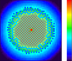
b)

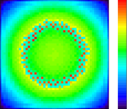
Figure 4: (Color online) Real-space density distribution of the light atoms for $U=J$ and $k_{\rm B}T=0.0001J$. The upper panel (a) corresponds to the trapping potential with $R=12.9a$ and the lower (b) to $R=17a$.

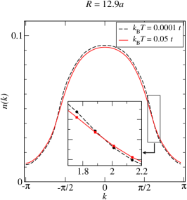
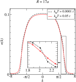
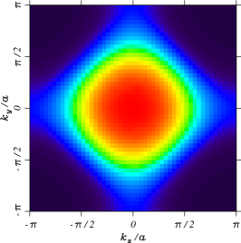
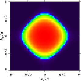
Figure 5: (Color online) Momentum distribution of the light atoms for the cases shown in Fig. 4. The upper row shows a comparison of cross sections along the $x$ axis for $k_{\rm B}T=0.0001J$ (dashed black line) and $k_{\rm B}T=0.005J$ (solid red line). The insets blows up the momentum distribution for atoms with energies close to the Fermi energy. The momentum distributions shown in the lower row were determined at $k_{\rm B}T=10^{-4}J$.

III.2 Heavy atom configurations

Since the heavy atoms are localized in the proposed approach, one cannot analyze their momentum distribution. Instead, we determine structure factors defined by Eq. 7. In particular, we are interested in how different density-wave-ordered patterns are reflected in the structure factor. It is well known from solid state physics that different orderings produce characteristic Bragg spectra. However, in the case of cold atoms the spectra are additionally affected by the confining potential that keeps the atoms inside the trap. Neglecting the interspecies interaction that may lead to phase separation or ordering, at low temperature, the heavy atoms occupy the bottom of the trap forming a circular region. Fourier transformation of such a configuration consists of a finite-width peak at position ${\bm{k}}=(0,0)$. Plotted in a region $(0,2\pi)\times(0,2\pi)$, the peak splits into four quarters which are visible in each corner [at ${\bm{k}}=(0,0),\ (0,2\pi),\ (2\pi,0)$ and $(2\pi,2\pi)$]. The peak itself simply results from a finite number of heavy atoms, since according to Eq. (7), $S({\bm{0}})$ is equal to the average concentration of the heavy atoms. The gathering of atoms in the center of the trap broadens it, as can be seen in Fig. 6.

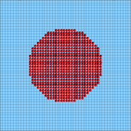
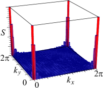
Figure 6: (Color online) Left panel: ground state real-space configuration of the heavy atoms in a harmonic trap. Right panel: corresponding structure factor.

When temperature or interaction moves the atoms to more peripheral areas, the peak width shrinks, finally taking on a delta-function-like form for a random distribution of atoms. It changes the spectral weight around ${\bm{k}}=(0,0)$ (and equivalent points), affecting the magnitude of the peaks representing ordered phases. This will be discussed in more detail below. Since we are mainly interested in patterns formed by the heavy atoms, we will neglect the ${\bm{k}}=(0,0)$ peak and focus on the remainder of the spectrum. Nevertheless, even in the presence of ordering, this peak is still the most pronounced feature of the spectrum.

Most of the results have been obtained at finite temperatures by means of the Monte Carlo method. These results can also be compared with zero-temperature local density approximation (LDA) results, which we now describe.

III.2.1 Zero temperature results: LDA

We construct the LDA at $T=0$ from the homogeneous, grand canonical phase diagram, where the ground state phases are given as a function of the chemical potentials of heavy and light atoms rom . The procedure is as follows. For each lattice site, we determine the local chemical potentials by subtracting the trap potential at that lattice site from a trial global chemical potential. The global chemical potential is then adjusted to produce the correct total number of heavy and light atoms in the trap. Next, using the local chemical potentials, we map out the homogeneous phase diagram for each site within the trap. Two sets of model parameters that give nontrivial configurations have been analyzed: $R=12.9a,\ U=J$ and $R=18.5a,\ U=5J$. In the former case, a checkerboard-type configuration is formed in the center of the trap, where the heavy atoms occupy, let us say, the black squares, and the light atoms are primarily on the white ones. The central part is surrounded by rings of different phases. In the latter case, the center of the trap is occupied by light atoms, while the heavy ones form a relatively thick ring composed mainly of various stripe phases. The spatial distributions have been obtained taking into account all possible periodic phases with unit cells consisting of no more than 4 lattice sites (in all possible shapes). The candidate phases are presented in Fig. 7.

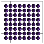
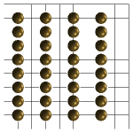
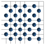
A)     B)     C)     D)     E)  

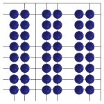
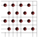
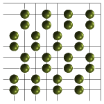
F)     G)     H)     I)  

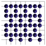
Figure 7: (Color online) All the configurations of the heavy atoms that have been taken into account in the LDA calculations. The letters correspond to different regions presented in Figs. 8A and 10A.

The zero-temperature LDA configurations are presented in the lower panels in Figs. 8A and 10A, where different letters correspond to different phases marked with the same identifying letters as in Fig. 7. The Bragg spectra presented in the upper panels in Figs. 8A and 10A are calculated in the following way: first, the positions of the $\delta$-function-type peaks are determined from the Fourier transforms of the configurations depicted in Fig. 7; then the relative spectral weight proportional to the fraction of the trap occupied by the corresponding phase is assigned to the given peaks. Finally, the peaks are slightly broadened to make the presentation more clear. This is necessary because the LDA does not know about the finite size of the system and hence always displays perfect delta-function peaks.

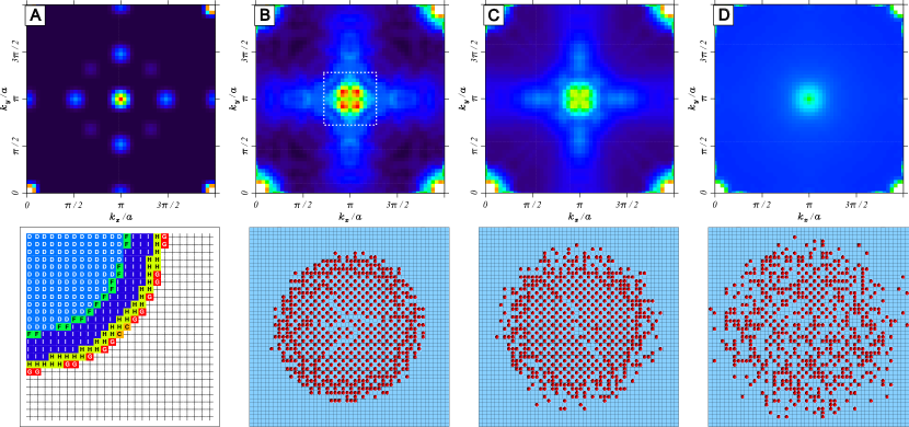
Figure 8: (Color online) Upper row: Fourier transforms of the spatial distributions of the heavy atoms; Lower row: corresponding spatial distributions for $U=J$. Figure A shows a transformation of a configuration obtained within the LDA. In the figure presenting the corresponding real-space configuration regions occupied by different phases are filled with different colors and marked by letters. Each letter stands for one configuration and the configurations are shown in Fig. 7. Figures B, C, and D correspond to results at finite temperature, $k_{\rm B}T=0.005J,\ 0.01J,$ and $0.05J$, respectively.

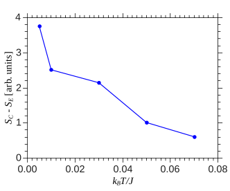
Figure 9: (Color online) Temperature dependence of the Bragg spectra in the center of the trap. More precisely, this figure shows $\sum_{\bm{k}}^{\prime}\bar{S}({\bm{k}})-\bar{S}(0,\pi)$ where the sum is calculated over the square marked by white dotted line in Fig. 8

It can be seen in Fig. 8A, that for $R=12.9a$ and $U=J$ a checkerboard phase occupies the central part of the trap. It leads to a highly pronounced peak at ${\bm{k}}=(\pi,\pi)$. Other phases give smaller peaks at $(\pi,\pi/2)$, $(\pi,0)$, $(2\pi/3,2\pi/3)$ (and points obtained by symmetry operations).

For $R=18.5a$ and $U=5J$ there are no heavy atoms in the center of the trap: they are distributed in a ring of some width with two different phases that have axial stripes on its innermost part. Since the stripes are invariant with respect to translations along the axis (neglecting the finite size of the system), all peaks are located at $k_{x}=0$ or $k_{y}=0$, namely at ${\bm{k}}=(0,\pi),\ (\pi,0),\ (0,\pm 2\pi/3)$ and $(\pm 2\pi/3,0)$. The outer part of the ring is densely filled with heavy atoms and its Fourier transform contributes to the peak at ${\bm{k}}=(0,0)$.

III.2.2 Finite temperatures: Monte Carlo

In order to investigate how temperature affects the patterns formed by the heavy atoms, Monte Carlo simulations have been carried out. For a sufficiently long MC run, a number of independent heavy atom configurations are generated. The length of a single MC run depends on the temperature and the model parameters (interaction, shape of the harmonic trap), but usually it is on the order of $10^{6}$ MC steps from which about $10^{3}-10^{4}$ independent configurations have been selected. For each configuration the Fourier transform has been calculated. Figs. 8BCD and 10BCD present results averaged over all configurations generated for a given set of model parameters. We need to comment about the averaging procedure. In an experiment, the Bragg spectra of a single configuration can be observed. However, in many cases the configuration (and the corresponding spectra) changes significantly between successive “snapshots”. In order to make our results independent of any particular distribution of the atoms, we decided to present results that can characterize the system at a given temperature and model parameters. Fourier transforms of very similar configurations often have similar shape, but may have different sign, depending on the details, e. g., on the phases of the order parameter for a checkerboard phase. Therefore, in Figs. 8BCD and 10BCD, we present averaged absolute values of the spectra, given by

$$\bar{S}({\bm{k}})=\frac{1}{MN}\sum_{m=1}^{M}\left|\sum_{i=1}^{N}w_{i,m}e^{i{\bm{k}}\cdot{\bm{R}}_{i}}\right|,$$ (8)

where $N$ and $M$ are the number lattice sites and the number of MC “snapshots”, respectively and $w_{i,m}$ is equal to 0 or 1, depending on whether site $i$ is occupied or empty in the $m$-th “snapshot”. Additionally, the resulting Bragg spectra are self averaged using rotational and reflection symmetries of the lattice and the trap. This means that the presented spectra are calculated as averages of $S(k_{x},k_{y})$, $S(k_{x},-k_{y})$, $S(-k_{x},k_{y})$, $S(-k_{x},-k_{y})$, $S(k_{y},k_{x})$, $S(k_{y},-k_{x})$, $S(-k_{y},k_{x}),$ and $S(-k_{y},-k_{x})$. Since we are not interested in the ${\bm{k}}=(0,0)$ peak (and equivalent peaks in the remaining corners), the false-color scales in Figs. 8 and 10 are chosen in such a way that (independent of the temperature) only the peaks resulting from ordering are correctly represented. But of course, the scale is kept the same in panels B, C, and D.

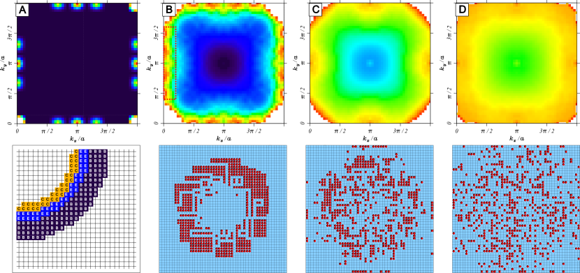
Figure 10: (Color online) The same as in Fig. 8, but for $U=5J$. Panels B, C, and D correspond to temperature $k_{\rm B}T=0.01J,\ 0.05J,$ and $0.15J$, respectively.

Figure 11: (Color online) Temperature dependence of the Bragg spectra at the edge of the trap: this figure shows $\sum_{\bm{k}}^{\prime}\bar{S}({\bm{k}})-\bar{S}(\pi,\pi)$ where the sum is calculated over the rectangle marked by red dotted line in Fig. 10

In the case presented in Fig. 8A (LDA, $U=J,R=12.9a$), most of the heavy atoms form a checkerboard configuration leading to a strong peak at ${\bm{k}}=(\pi,\pi)$. In the peripheral areas, the concentration of heavy atoms increases and they form more dense patterns, which in turn, lead to less pronounced peaks. One can notice that the central peak in Fig. 8B is fourfold split. This results from an imperfection of the checkerboard ordering of the heavy atoms. This can be explained from an analysis of the LDA: the effective chemical potential varies continuously when the distance from the center of the trap increases. Hence one expects that the density of atoms (both light and heavy) should also vary in a continuous way. However, in some regions, the checkerboard ordering minimizes the energy, hence in that ordered region the density (at least of the heavy atoms) is constant. A competition between these two tendencies leads to flaws in the center of the trap. Due to topological reasons, such a crack has to run across the entire ordered area. Then the question is why the fourfold split is not visible in the LDA results? This is connected with the maximum size of the unit cell taken into account in the LDA calculations. The $4$ site unit cell is too small to describe a large checkerboard area with a single line defect, but by using a larger unit cell, one should see such a configuration.

As can be expected, the ordering is reduced when the temperature increases and so are the corresponding features in the Bragg spectra. Figs. 8C and 8D illustrate how the multi-peak structure is smoothed out by destroying the real-space ordering. In order to describe this process in a more quantitative way, we calculated how the spectral weight of the central peak(s) decreases with increasing temperature. Figure 9 shows the spectral weight in a region $(0.75\pi\leq k_{x}\leq 1.25\pi)\times(0.75\leq k_{y}\leq 1.25\pi)$ (marked by the white square in Fig. 8A) as a function of temperature. The plot is shifted in such a way that the weight at ${\bm{k}}=(\pi,0)$ is equal to zero. The shift is necessary since with increasing temperature less and less weight is attributed to the peak at ${\bm{k}}=(\pi,0)$, which increases the reference level more than should result from the reduction of the central peak (this effect is especially visible in Fig. 10, where the color around $(\pi,\pi)$ becomes very bright at high temperature).

IV Summary

In this paper, we have examined two simple experimental probes that can reveal information about ordered density wave phases in mixtures of light and heavy fermionic atoms (or equivalently light fermionic and heavy “hard core” bosonic atoms) on an optical lattice. Namely, we examined the momentum distribution function, which comes from a time-of-flight expansion experiment and the Bragg scattering signal that would come from scattered optical light that scatters off of the density wave pattern.

The momentum distribution function does not provide significant information about various ordered density wave phases, but it does provide some intuition about phase separated states. In particular, as the distribution flattens and broadens, one has an indication of phase separation setting in. Furthermore, if the heavy atoms surround the lights and confine the light atoms with essentially a hard wall boundary condition, then the momentum distribution function develops a sharp dimple at low momentum which does provide a characteristic shape signalling that form of phase separation.

Bragg scattering is much more effective at showing the presence of ordered density wave phases, as new Bragg reflection “spots” appear at appropriate ordering vectors for the different types of order present in the sample. The weight underneath these peaks is proportional to the strength of the ordering, and to the volume of regions which are ordered, and hence they can be used for accurate low-temperature thermometry of these systems. As $T$ is lowered, the weight in the peaks grows and can be calibrated via numerical calculations to produce an appropriate temperature of the system.

One caveat of this work, however, is that one must cool the mixture down to a low enough temperature that the ordering appears in the system. Typically, this requires a temperature at least as low as about 1/40th of the bandwidth, and often substantially lower. This is an aggressively low temperature with current cooling technology, but hopefully can be reached as it becomes easier to manipulate entropy distributions within trapped atomic systems. Finally, we also should note that direct in situ imaging via apparatus like the quantum gas microscope would provide even more convincing pictures of the ordered phases, and the fluctuations about that order, than the above proposed methods, but we are not aware of any plans to examine these kinds of mixtures with such machines in the near term.

- (1) M. Rigol and A. Muramatsu, Phys. Rev. A 70, 043627 (2004).
- (2) D. A. Butts and D. S. Rokhsar, Phys. Rev. A 55, 4346 (1997).
- (3) N. H. Marcha, L. M. Nietoc, and M. P. Tosi, Phys. B: Condens. Matter 293, 308 (2001).
- (4) M. M. Maśka, R. Lemański, J.K. Freericks, and C.J. Williams, Phys. Rev. Lett. 101, 060404 (2008).
- (5) W. S. Bakr, J.I. Gillen, A. Peng, S. Foelling, M. Greiner Nature 462, 74 (2009).
- (6) L. M. Falicov and J. C. Kimball, Phys. Rev. Lett. 22, 997 (1969).
- (7) C. Ates and K. Ziegler, Phys. Rev. A 71, 063610 (2005).
- (8) K. Byczuk and D. Vollhardt, Phys. Rev. B 77, 235106 (2008); Ann. Phys. 18, 622 (2009).
- (9) M. Iskin and J. K. Freericks, Phys. Rev. A 80, 053623 (2009).
- (10) M. M. Maśka, K. Czajka, Phys. Rev. B 74, 035109 (2006); M. M. Maśka, K. Czajka, phys. stat. sol. 242, 479 (2005).
- (11) Daw-Wei Wang, Phys. Rev. A 80, 063620 (2009).
- (12) G. Birkl, M. Gatzke, I. H. Deutsch, S. L. Rolston, and W. D. Phillips, Phys. Rev. Lett. 75, 2823 (1995); Matthias Weidemüller, Axel Görlitz, Theodor W. Hänsch, and Andreas Hemmerich, Phys. Rev. A 58, 4647 (1998); Philipp T. Ernst, Sören Götze1, Jasper S. Krauser, Karsten Pyka, Dirk-Sören Lühmann, Daniela Pfannkuche, and Klaus Sengstock, Nature Physics 6, 56 (2010).
- (13) T. A. Corcovilos, S. K. Baur, J. M. Hitchcock, E. J. Mueller, and R. G. Hulet, Phys. Rev. A 81, 013415 (2010).
- (14) J. K. Freericks, E. H. Lieb, and D. Ueltschi, Commun. Math. Phys. 227, 243 (2002).
- (15) G. I. Watson and R. Lemański, J. Phys. Condens. Matter 7, 9521 (1995); R. Lemański, J. K. Freericks and G. Banach, J. Stat. Phys. 116, 699 (2004).