Flying microwave qubits with nearly perfect transfer efficiency

Abstract

We propose a procedure for transferring the state a microwave qubit via a transmission line from one resonator to another resonator, with a theoretical efficiency arbitrarily close to 100%. The emission and capture of the microwave energy is performed using tunable couplers, whose transmission coefficients vary in time. Using the superconducting phase qubit technology and tunable couplers with maximum coupling of 100 MHz, the procedure with theoretical efficiency $\eta=0.999$ requires a duration of about 400 ns (excluding propagation time) and an ON/OFF ratio of 45. The procedure may also be used for a quantum state transfer with optical photons.

I Introduction

Rapid progress in experiments with superconducting qubits sc-qubits confirms their importance for quantum information processing. However, all such experiments so far are confined to one chip inside a dilution refrigerator, without a possibility to transfer quantum information from chip to chip or over a longer distance between the refrigerators. In particular, the superconducting experiment on the Bell inequality violation Bell has been done with the locality loophole. A natural way of passing quantum information from site to site is by using “flying qubits” represented by single photons (or more precisely, superpositions of one and zero photons). For a superconducting qubit we may think about emission of a microwave photon, which propagates through a lossless superconducting waveguide and is then “captured” by another qubit. The technology of superconducting qubits coupled to microwave resonators based on coplanar waveguides is now well developed.coplanar Since the resonators have better coherence time than the qubits, it may be beneficial to transfer quantum information between two resonators instead of coupling qubits to the transmission line directly.

The transfer of quantum information from site to site may seem much easier in optics; however, this is not the case. Even though optical photons easily propagate in fibers, it is not easy to capture a photon for further information processing, without destroying it. An important idea is to use trapping of photon states in atomic ensembles. Lukin In this way entanglement between remote atomic ensembles can be established and then used to transfer quantum information; however, general processing of the quantum information by linear optics means KLM is problematic because of its indeterministic nature. Some other approaches (e.g., Refs. other, ) may also be useful for the transfer of quantum information over large distances, but in any case such transfer is not simple.

A promising idea for a quantum state transfer between two identical oscillators of either optical or microwave range of frequency via a transmission line was put forward by Jahne, Yurke, and Gavish. Yurke In their scheme the coupling between the emitting oscillator and the transmission line changes in time. It was shown Yurke that with a specific time dependence of the coupling, the fidelity $F$ of the transfer can be made arbitrarily close to 100%. Unfortunately, the required ON/OFF ratio for the coupler is quite large, ON/OFF$\gg 1/(1-F)$, and the duration of the procedure $T$ (excluding the propagation time) is quite long, $T\gg Q_{\rm min}^{\rm em}/[\omega(1-F)]\ln(1-F)^{-1}$, where $\omega$ is frequency of the oscillators and $Q_{\rm min}^{\rm em}\gg 1$ is the minimum “loaded” quality factor of the emitting oscillator corresponding to its maximum coupling to the transmission line. These requirements make this scheme impractical for a high-fidelity ($1-F\simeq 10^{-3}$) transfer between superconducting qubits or microwave resonators, even though tunable couplers for superconducting qubits have been demonstrated experimentally. tunable ; Bialczak A search for practical schemes for such transfer is currently under way.Gal-Geller ; Cleland-comm

In this paper we consider a modification of the above scheme with the primary difference being the use of tunable couplers for both the emitting and receiving resonators. This drastically reduces the required ON/OFF ratio and duration of the procedure: ON/OFF$\sim 1/\sqrt{1-F}$, $T\sim[Q_{\min}/\omega]\ln(1-F)^{-1}$, where $Q_{\min}\gg 1$ corresponds to the maximum available coupling of both resonators with the transmission line. Actually, instead of using the amplitude fidelity $F$, we will characterize the transfer by the energy efficiency $\eta=F^{2}$. In the above formulas $F$ can be replaced with $\eta$ because $1-F\approx(1-\eta)/2$. With these improved requirements, we believe the information transfer between superconducting qubits may become practical.

As a tunable coupler we consider the experimentally realized inductive coupler of Ref. Bialczak, . In the analysis we assume weak coupling (large $Q$-factors of the resonators) and slow variation of the coupling compared to the resonator frequency. This allows us to neglect field propagation within the resonators and consider evolution of only one standing-wave mode in each resonator. The main idea of the procedure is very simple: we tune the couplers to cancel the back-reflection into the transmission line from the receiving coupler.

The next section is an overview of the work: we describe the system and the procedure, derive main results in a simple approximate way, and compare our system and results with those of Ref. Yurke, . In Section III we calculate the $S$-parameters (transmission and reflection amplitudes) for a tunable coupler of Ref. Bialczak, . Section IV presents a quantitative analysis of the procedure and estimates for the technology of superconducting phase qubits. Section V is a conclusion. Section III and a part of Sec. IV assume a particular superconducting qubit system. Most of results of Secs. II and IV are applicable to any system with realizable tunable couplers between a resonator and a transmission line (hopefully, such tunable couplers between an optical cavity and a fiber waveguide will be developed in future).

II Overview: system, main idea, and approximate results

Our goal is to transfer a quantum state between two microwave resonators via a transmission line (Fig. 1). This is done by varying in time the coupling between the resonators and the transmission line. Assuming sufficiently slow evolution (high-$Q$ resonators and slow change of the coupling) we consider only one mode per resonator and assume the same frequency $\omega$ of these modes (the effect of a frequency mismatch will be discussed in Sec. IV). Since in our simple case the quantum language essentially coincides Yurke ; Walls-Milburn ; Yurke-84 with the classical language (the classical field amplitudes should be associated with annihilation operators in the Heisenberg picture), we will basically discuss a classical field transfer between the resonators. The resulting microwave phase in the receiving resonator (which corresponds to a qubit phase) depends on the duration of propagation through the transmission line. In our procedure we do not attempt to control this phase and characterize the quality of the procedure by the energy efficiency $\eta$. For simplicity we assume a lossless and dispersionless transmission line and lossless resonators, so that the relative energy loss $1-\eta$ is due to an imperfect transmission/capture of the wave only.

Figure 1: Our goal is to pass a classical microwave energy from one resonator to another one via a transmission line. Conceptually, this is done by varying in time transmission amplitudes of “barriers” (tunable couplers) separating the resonators (half wavelength or quarter wavelength in size) and the long transmission line.

The main idea of our construction for a nearly perfect transfer is the following. Suppose a microwave (voltage) waveform $A(t)\,e^{i\omega t}$ is incident to the receiving coupler from the transmission line (Fig. 1). The time dependence of the receiving coupler parameters is chosen in the way, which eliminates the wave reflected from the receiving coupler back into the transmission line. This is done by arranging exact cancellation (destructive interference) between the reflected wave and the transmitted part of the wave $B(t)\,e^{i\omega t}$ from the receiving resonator. If the reflection back into the transmission line is canceled, then all of the microwave power is collected in the receiving resonator – this is exactly our goal. Instead of varying in time the receiving coupling to achieve a perfect cancellation of the refection, it is also possible to keep it fixed, but vary the emitting coupling, designing a specific $A(t)$ for a perfect cancellation. In a general case both the emitting and receiving coupler parameters can be varied in time in accordance with each other to satisfy just one equation: cancellation of the reflection. Actually, this is a complex-number equation because of an amplitude and a phase; however, we will see later that in the case of equal resonator frequencies and weak coupling the phase relation is satisfied automatically, so we are left with only one real equation to be satisfied. In our particular construction we vary only the emitting coupling in the first part of the procedure, while keeping maximum the receiving coupling, and do it in the opposite way in the second part of the procedure: keep the emitting coupling maximum and vary the receiving coupling. The durations of the two parts are approximately equal.

The perfect reflection cancellation is obviously impossible at the beginning of the procedure, because it should take time to build up the microwave amplitude $B(t)$ in the receiving resonator. The microwave reflected back into the transmission line during the build-up time is irrecoverably lost (it may actually lead to multiple reflections, but we treat it as being lost – see discussion later). This means that we should design the waveform envelope $A(t)$ to be very small during this initial period (see Fig. 2), while after the build-up is finished, $A(t)$ can start increasing rapidly. Let us choose it constant, $A(t)=A_{0}$, during the build-up and crudely estimate the energy loss. Notice that we shift the time origins at the emitter and receiver by the propagation time, so that $t$ means both the emitting and receiving time. Also notice that $A(t)$ can be assumed real.

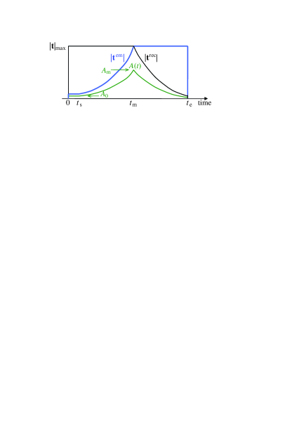
Figure 2: (Color online) Sketches of the assumed time dependence $|{\bf t}^{\rm em}(t)|$ of the transmission amplitude of the emitting coupler (blue), transmission amplitude $|{\bf t}^{\rm rec}(t)|$ of the receiving coupler (black), and the wave amplitude $A(t)$ incident to the receiving coupler from the transmission line (green). The voltage amplitude $A(t)$ is constant ($A_{0}$) during the build-up period $0<t<t_{\rm s}$, then increases exponentially until time $t_{\rm m}$ at which $|{\bf t}^{\rm em}|$ reaches the maximum available value $|{\bf t}|_{\rm max}$, and after that $A(t)$ decreases exponentially until the end of the process $t_{\rm e}$. The receiving coupling $|{\bf t}^{\rm rec}|$ is kept at the maximum value $|{\bf t}|_{\rm max}$ at $t<t_{\rm m}$, while at $t>t_{\rm m}$ the emitting coupling $|{\bf t}|^{\rm em}$ is kept at the maximum $|{\bf t}|_{\rm max}$. The ratio of couplings $|{\bf t}^{\rm em}/{\bf t}^{\rm rec}|$ is chosen to cancel the back-reflection into the transmission line at any time after $t_{\rm s}$.

During the build-up period the transmission amplitude ${\bf t}^{\rm rec}$ of the receiving coupler is kept at the maximum available value ${\bf t}_{\rm max}$, which is still small, $|{\bf t}|_{\rm max}\ll 1$ (boldface is used for ${\bf t}$ to distinguish it from time; we will see later that the phase of complex ${\bf t}$ is fixed). To start the perfect reflection cancellation we need the wave amplitude $|B|$ in the resonator to become $|A_{0}/{\bf t}_{\rm max}|$; this will happen at the “start” time $t_{\rm s}\sim\tau_{\rm bu}\equiv\tau_{\rm rt}/|{\bf t}|_{\rm max}^{2}$, where $\tau_{\rm bu}$ is the time constant of the build-up process, $t_{\rm s}\neq\tau_{\rm bu}$ because the resonator leaks through the coupler, and $\tau_{\rm rt}$ is the round-trip time of the wave in the resonator. For the lowest-frequency mode

$$\tau_{\rm rt}\approx 2\pi/\omega\hskip 8.5359pt{\rm or}\hskip 8.5359pt\tau_{\rm rt}\approx\pi/\omega$$ (1)

for a $\lambda/2$ (half-wavelength) resonator or a $\lambda/4$ resonator, respectively (these equations are not exact because the coupler may affect the boundary condition). Notice that our definition of the build-up time constant $\tau_{\rm bu}$ has a direct relation to the resonator $Q$-factor due to the coupler: in absence of the incoming wave the fraction $|{\bf t}|^{2}$ of resonator energy would be lost every $\tau_{\rm rt}$, therefore $Q=\omega\tau_{\rm rt}/|{\bf t}|^{2}$, and so $\tau_{\rm bu}=Q_{\rm min}/\omega$ (in this derivation we implicitly assumed the same wave impedance $R$ in the resonator and in the transmission line). Since the travelling wave $A_{0}$ carries the power $|A_{0}|^{2}/2R$, the energy loss during the build-up period $t_{\rm s}$ is $\sim|A_{0}|^{2}\tau_{\rm bu}/R$, which should be later compared with the total transmitted energy.

After $t_{\rm s}$ the transmitted energy is no longer being lost, and $A(t)$ may increase as fast as $A_{0}\exp[(t-t_{\rm s})/2\tau_{\rm bu}]$. A simple way to derive this formula is by applying time reversal to the “no-reflection” procedure, which converts it into a “no incident wave” case, corresponding to a leaking resonator. In such a case the wave amplitude in the resonator decreases as $\exp(-\omega t/2Q)$ [the energy decreases as $\exp(-\omega t/Q)$], and the leakage amplitude in the transmission line has the same time dependence. Therefore for the absence of reflection we need $A(t)\propto\exp(\omega t/2Q)$, and for the assumed maximum coupling ($Q_{\rm min}=\omega\tau_{\rm bu}$) we get $A(t)\propto\exp(t/2\tau_{\rm bu})$. The application of time reversal also proves that the wave in the receiving resonator automatically accumulates with a proper phase for the reflection cancellation.

Exponentially increasing $A(t)$ requires a strong increase of the emitting resonator coupling (slightly faster than exponential), so this process can last only until some time $t_{\rm m}$, when the emitting coupling reaches its physical limit (see Fig. 2). The reflection cancellation can still be achieved after this time by decreasing the receiving coupling. Assuming the same maximum transmission $|{\bf t}|_{\rm max}$ and the same $\tau_{\rm rt}$ for the emitting and receiving resonators, we find that after $t_{\rm m}$ the transmitted amplitude becomes exponentially decreasing, $A(t)\propto\exp(-t/2\tau_{\rm bu})$, with the same time constant as for the increasing part. To maintain the reflection cancellation, the receiving coupling ${\bf t}^{\rm rec}$ should then be decreased in time slightly faster than $\propto\exp(-t/2\tau_{\rm bu})$, since the amplitude $B(t)$ in the receiving resonator continues to grow.

If we end the procedure at a finite time $t_{\rm e}$, then there will be some energy left untransmitted/unreceived. From the symmetry, if we choose $t_{\rm e}-t_{\rm m}\approx t_{\rm m}-t_{\rm s}$, then this energy loss will be comparable to the energy loss $\sim|A_{0}|^{2}\tau_{\rm bu}/R$ during the build-up period $t_{\rm s}$. Since the total transmitted energy is approximately $|A_{0}|^{2}\exp[(t_{\rm m}-t_{\rm s})/\tau_{\rm bu}]\,\tau_{\rm bu}/R$, the relative loss is $1-\eta\sim\exp[-(t_{\rm m}-t_{\rm s})/\tau_{\rm bu}]$. Therefore, for an almost perfect efficiency $\eta$, the total duration of the procedure, $t_{\rm e}\approx 2(t_{\rm m}-t_{\rm s})$, should be crudely

$$t_{\rm e}\simeq 2\,\tau_{\rm bu}\ln\frac{1}{1-\eta},\,\,\,\tau_{\rm bu}=\frac{\tau_{\rm rt}}{|{\bf t}|_{\rm max}^{2}}=\frac{Q_{\rm min}}{\omega}.$$ (2)

The required ON/OFF ratio $|{\bf t}|_{\rm max}/|{\bf t}|_{\rm min}$ for the receiving coupler can be estimated as $\sqrt{2}A(t_{\rm m})/A(t_{\rm e})=\sqrt{2}\exp[(t_{\rm e}-t_{\rm m})/2\tau_{\rm bu}]$, where the factor $\sqrt{2}$ is needed because the energy in the receiving resonator at time $t_{\rm m}$ is approximately half of its energy at time $t_{\rm e}$. An estimate for the emitting coupler is similar because $A(t_{\rm s})\sim A(t_{\rm e})$. Therefore, the requirement is crudely

$${\rm ON/OFF}\simeq\frac{\sqrt{2}}{\sqrt{1-\eta}}.$$ (3)

Equations (2) and (3) are the main approximate results for our procedure; the exact results will be presented in Sec. IV. A quick estimate using $|{\bf t}|_{\rm max}^{2}\simeq 10^{-2}$, $\omega/2\pi=6$ GHz, $\tau_{\rm rt}=\pi/\omega$, and $\eta=0.999$, gives numbers quite encouraging for an experiment with superconducting qubits: $t_{\rm e}\simeq 120$ ns and ON/OFF $\simeq$ 45.

Now let us discuss the differences between our work and Ref. Yurke, , and the reason why we obtained so much better results for the duration $t_{\rm e}$ and ON/OFF ratio. Most importantly, in Ref. Yurke, only the emitting coupling ${\bf t}^{\rm em}$ is modulated in time (receiving coupling ${\bf t}^{\rm rec}$ is fixed), so that in the language of our Fig. 2 the amplitude $A(t)$ continues to increase exponentially after $t_{\rm m}$, until the emitting resonator is practically empty. Then, since at $t_{\rm e}$ the ratio of wave amplitudes in the emitting and receiving resonators should be $\sim\sqrt{1-\eta}$ (the energy ratio is $\sim 1-\eta$), the ratio of transmissions is ${\bf t}^{\rm rec}/{\bf t}^{\rm em}_{\rm max}\sim\sqrt{1-\eta}$. Similarly, at $t_{\rm s}$ there should be the opposite relation of the wave amplitudes, and therefore ${\bf t}^{\rm em}_{\rm min}/{\bf t}^{\rm rec}\sim\sqrt{1-\eta}$. As a result, the required ON/OFF ratio is ${\bf t}^{\rm em}_{\rm max}/{\bf t}^{\rm em}_{\rm min}\sim 1/(1-\eta)$, which is much larger than our result (3). Since the receiving resonator amplitude increases by $\sim 1/\sqrt{1-\eta}$ times between $t_{\rm s}$ and $t_{\rm e}$, the duration of the procedure can be estimated as $t_{\rm e}\simeq(Q^{\rm rec}/\omega)\ln(1-\eta)^{-1}\sim[Q^{\rm em}_{\rm min}/\omega(1-\eta)]\ln(1-\eta)^{-1}$. This is $\sim 1/(1-\eta)$ times longer than our result (2) for the same $Q_{\rm min}^{\rm em}$.

Actually, the requirements for the procedure duration and ON/OFF ratio reported in Ref. Yurke, are even stronger: there are inequalities with “much greater” signs instead of the signs “comparable” in our estimates. The strategy is also different. The idea of reflection cancellation is not mentioned in Ref. Yurke, and our initial build-up period $t<t_{\rm s}$ is absent. Instead, the result is obtained by a formal optimization of the fidelity using the Euler-Lagrange equation. In this case the reflection cancellation is not exact. However, this is a relatively minor difference between Ref. Yurke, and our work. Even though the idea of reflection cancellation is not discussed in Ref. Yurke, , it is essentially there.

As one more difference, the scheme of Ref.  Yurke, assumes a circulator placed in between the resonators, so that the back-reflected wave is diverted and fully absorbed. In our derivation we essentially analyze the same situation treating the reflected wave as a loss; however, we do it with a different reasoning, not assuming a circulator. Formally, we can assume a very long transmission line, so that the reflected wave does not play any role. In a real experiment this is impossible, and the reflected wave leads to multiple reflections from the two couplers, which greatly complicates the analysis. However, there is a simple way to show that the multiple reflections do not change the efficiency $\eta$ significantly. Let us separate the wave amplitudes at time $t_{\rm s}$ into two parts: the result of the simple analysis for which $B(t_{\rm s})=-A_{0}/{\bf t}_{\rm max}$ and the remaining part. Then using the system linearity we can analyze the further evolution of both parts separately and add their contributions at the end time $t_{\rm e}$. Since the reflection is fully cancelled in our usual procedure after $t_{\rm s}$, the evolution of this part remains the same as in the simple analysis. For the remaining part let us use the energy conservation. If the length of the transmission line is not resonant with the frequency $\omega$ (we assume this case), then the energy of the remaining wave part cannot be larger than on the order of $|A_{0}|^{2}t_{\rm s}/R\sim E_{\rm in}(1-\eta)$, where $E_{\rm in}$ is the initial energy of the emitting resonator. The transfer efficiency is decreased if this wave gives an anti-phase contribution at the receiving resonator at time $t_{\rm e}$. Instead of considering the receiving resonator at $t_{\rm e}$, it is easier to use conservation of the total energy and estimate the energy at $t_{\rm e}$ in the emitting resonator and the transmission line. Even if the two wave contributions (from simple analysis and due to multiple reflections) are added there in-phase, the energy loss cannot be larger than twice the sum of the corresponding energies, so it is still on the order of $E_{\rm in}(1-\eta)$. Therefore even in the worst-case scenario the inefficiency $1-\eta$ cannot increase more than few times due to the effect of multiple reflections. Moreover, such increase requires an unlucky phasing of the multiple reflections, while on average $\eta$ is not decreased by their contribution. This is why we neglect multiple reflections in our analysis and consider the reflected wave as being lost.

From the above analysis based on linearity and energy conservation it is clear that the initial period $t_{\rm s}$ is actually not needed. We can start the procedure of reflection cancellation from $t=0$ just pretending that the needed amplitude $A_{0}/{\bf t}_{\rm max}$ is already in the receiving resonator. The energy loss at the start of the procedure will be then only few times larger, and this can be compensated by a slight decrease of $A_{0}$. The time dependence of ${\bf t}^{\rm em}$, ${\bf t}^{\rm rec}$, and $A$ on Fig. 2 in this case will be fully symmetric about the middle point $t_{\rm m}$. Even though the initial period $t_{\rm s}$ is not necessary, we keep it in our analysis for conceptual simplicity.

III $S$-parameters for inductive tunable coupler and $Q$-factor

The idea described in the previous section can be applied to various systems which permit realization of tunable “barriers” between standing-wave modes in resonators and a propagating mode in a transmission line. However, in this paper we will focus on a particular technology developed for superconducting phase qubits, Bialczak which can be used to transfer microwave qubits between two superconducting coplanar waveguide (or microstrip) resonators. In particular, in this section we will calculate the transmission and reflection amplitudes ${\bf t}$ and ${\bf r}$ for the tunable coupler of Ref. Bialczak, , assuming that this coupler connects two coplanar waveguides (or microstrips). The readers interested in other realization (optical, etc.) can skip this section and go directly to Sec. IV, in which the transfer procedure of Sec. II is analyzed in more detail.

Notice that the terminology of $S$-parameters (scattering matrix elements) is the same in microwave technology and in quantum mechanics. Instead of the notation $S_{11}$, $S_{12}$, etc., we use a more transparent notation $S=\left(\begin{array}[]{cc}{\bf r}_{1}&{\bf t}_{2}\\ {\bf t}_{1}&{\bf r}_{2}\end{array}\right)$, where the subscript indicates that the incident wave came from the left (side 1) or from the right (side 2) – see Fig. 3. In the usual case of equal wave impedances from both sides, $R_{1}=R_{2}=R$, the $S$-matrix should be unitary because of the energy conservation, which means $|{\bf t}_{1}|^{2}+|{\bf r}_{1}|^{2}=|{\bf t}_{2}|^{2}+|{\bf r}_{2}|^{2}=1$ and ${\bf r}_{2}/{\bf r}_{1}^{*}=-{\bf t}_{2}/{\bf t}_{1}^{*}$ (so that necessarily $|{\bf t}_{2}|=|{\bf t}_{1}|$ and $|{\bf r}_{2}|=|{\bf r}_{1}|$). The reciprocity condition in the usual case (same for microwaves and in quantum mechanics) gives ${\bf t}_{2}={\bf t}_{1}$ (so we will use ${\bf t}$ without a subscript), and therefore the general form is

$$S=\left(\begin{array}[]{cc}{\bf r}_{1}&{\bf t}\\ {\bf t}&-{\bf r}_{1}^{*}{\bf t}/{\bf t}^{*}\end{array}\right),\,\,\,|{\bf t}|^{2}+|{\bf r}_{1}|^{2}=1.$$ (4)

Notice that if the coupler is symmetric, then ${\bf r}_{1}={\bf r}_{2}$, and this is possible only if ${\bf t}$ and ${\bf r}$ are shifted by $\pm 90$ degrees; in other words the ratio ${\bf t}/{\bf r}$ should be purely imaginary. In a general asymmetric case ${\bf t}^{2}/{\bf r}_{1}{\bf r}_{2}$ is negative-real, and therefore ${\bf t}/\sqrt{{\bf r}_{1}{\bf r}_{2}}$ is purely imaginary.

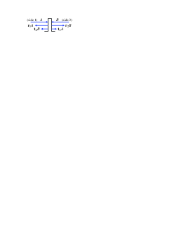
Figure 3: Notations for the scattering matrix.

Now let us consider the tunable coupler of Ref. Bialczak, (for other ideas used for superconducting qubits see Ref. tunable, ), and for simplicity Pinto let us describe it as an inductive coupler (Fig. 4) with inductances $L_{1}$ and $L_{2}$, and mutual inductance $M$. In the experiment Bialczak $L_{1}$ and $L_{2}$ are practically constant, while $M$ is tunable and small, $M^{2}\ll L_{1}L_{2}$. The actual circuitBialczak is more complex than in Fig. 4. The effective coupling inductance $M$ consists of two contributions: a fixed negative geometrical mutual inductance and a tunable positive Josephson inductance of a shared Josephson junction, which is tuned by controlling a bias current. In spite of simplicity, the model of Fig. 4 is a good description, as confirmed by the experimental results Bialczak and quantum analysis. Pinto Parasitic elements like distributed stray capacitance surely make the model more complicated; however, in the assumed weak-coupling limit their possible effect is only a slight change of the transmission and reflection amplitudes.

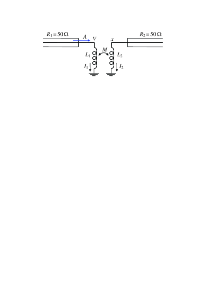
Figure 4: The tunable coupler consisting of inductances $L_{1}$ and $L_{2}$ coupled by a tunable mutual inductance $M$. Incoming wave amplitude is $A$ (voltage), the voltages across the inductors are $V$ and $x$, and the transmission amplitude is ${\bf t}=x/A$.

As a reminder, if a microwave transmission line is terminated with a short, then ${\bf r}=-1$ (the voltage changes sign because the voltage is zero at the short), while if it is terminated with a break, then ${\bf r}=1$ (because then the current is zeroed). The short (very small impedance) or break (very large impedance) should be compared with the wave impedance of the transmission line $R\simeq 50\,\Omega$. We mostly consider the case of large inductances $L_{1,2}$ in the coupler, $\omega L_{1,2}\gg R$, and weak coupling, $M^{2}\ll L_{1}L_{2}$, so that ${\bf r}_{1}\approx{\bf r}_{2}\approx 1$. The transmission amplitude ${\bf t}$ is therefore almost purely imaginary. Let us first find ${\bf t}$ in this high-impedance weak-coupling approximation, and then find it in a general case.

Assume that there is a voltage wave $Ae^{i\omega t}$ incident from the left, and there is nothing incident from the right. Since ${\bf r}_{1}\approx 1$, the voltage across $L_{1}$ is $V=2Ae^{i\omega t}$ (we will often omit $e^{i\omega t}$ by using the phasor representation), and the current in $L_{1}$ is $I_{1}=V/i\omega L_{1}$. It is important that the voltage across $L_{2}$ is not $VM/L_{1}$ because $L_{2}$ is loaded by a small resistance $R$. Let us denote the voltage across $L_{2}$ as $x$; then the current in the outgoing transmission line is $x/R$, and the current in $L_{2}$ is the same with opposite sign: $I_{2}=-x/R$. Then from the standard equation for coupled inductors (a transformer)

$$x=M(i\omega I_{1})+L_{2}(i\omega I_{2})=i\omega M\,\frac{V}{i\omega L_{1}}-i\omega L_{2}\,\frac{x}{R}$$ (5)

we find $x=(VM/L_{1})/(1+i\omega L_{2}/R)$. Since we assume $\omega L_{2}\gg R$, this means $x=(VM/L_{1})(R/i\omega L_{2})$. Finally, using the relation $V=2A$, we find the transmission amplitude ${\bf t}=x/A$ in the high-impedance weak-coupling approximation:

$${\bf t}=-i\,\frac{2MR}{\omega L_{1}L_{2}},\,\,\,\,{\bf r}_{2}={\bf r}_{1}=1-\frac{|{\bf t}|^{2}}{2},$$ (6)

where the term $|{\bf t}|^{2}/2$ is included to satisfy $|{\bf t}|^{2}+|{\bf r}|^{2}=1$ in the leading order (actually, neglected imaginary contributions to ${\bf r}_{2}$ and ${\bf r}_{1}$ can be larger than $|{\bf t}|^{2}$, but they are not so important).

Now let us consider a general case with arbitrary ratios $\omega L_{1}/R_{1}$, $\omega L_{2}/R_{2}$, and $M^{2}/L_{1}L_{2}$, and possibly different wave impedances $R_{1}$ and $R_{2}$ of the two transmission lines. In quantum mechanics $R_{1}\neq R_{2}$ corresponds to different potential energies or effective masses at the two sides. In this case the scattering matrix $S$ is no longer unitary. Instead, the matrix $\tilde{S}=\left(\begin{array}[]{cc}{\bf r}_{1}&{\bf t}_{2}\sqrt{R_{2}/R_{1}}\\ {\bf t}_{1}\sqrt{R_{1}/R_{2}}&{\bf r}_{2}\end{array}\right)$ is unitary; this still follows from the conservation of energy. The reciprocity condition is now ${\bf t}_{1}\sqrt{R_{1}/R_{2}}={\bf t}_{2}\sqrt{R_{2}/R_{1}}$, which leads to the following general form of the $S$-matrix:

$$S=\left(\begin{array}[]{cc}{\bf r}_{1}&{\bf t}_{1}R_{1}/R_{2}\\ {\bf t}_{1}&-{\bf r}_{1}^{*}{\bf t}_{1}/{\bf t}^{*}_{1}\end{array}\right),\,\,\,|{\bf t}_{1}|^{2}\frac{R_{1}}{R_{2}}+|{\bf r}_{1}|^{2}=1.$$ (7)

Notice that $|{\bf r}_{1}|=|{\bf r}_{2}|$ but $|{\bf t}_{1}|\neq|{\bf t}_{2}|$.

The derivation for ${\bf t}_{1}$ and ${\bf r}_{1}$ is now slightly different because the voltage $V=A(1+{\bf r}_{1})$ is unknown, so we have a system of two equations:

$$x=i\omega M\frac{(1-{\bf r}_{1})A}{R_{1}}-i\omega L_{2}\frac{x}{R_{2}},$$ (8)

$$(1+{\bf r}_{1})A=i\omega L_{1}\frac{(1-{\bf r}_{1})A}{R_{1}}-i\omega M\frac{x}{R_{2}}$$ (9)

(notice that now $I_{1}\neq V/i\omega L_{1}$), from which we find ${\bf t}_{1}=x/A$ and ${\bf r}_{1}$:

$${\bf t}_{1}=-i\,\frac{2MR_{2}}{\omega(L_{1}L_{2}-M^{2})}$$

$$\times\left[1-i\frac{R_{2}L_{1}+R_{1}L_{2}}{\omega(L_{1}L_{2}-M^{2})}-\frac{R_{1}R_{2}}{\omega^{2}(L_{1}L_{2}-M^{2})}\right]^{-1},\,\,\,$$ (10)

$${\bf r}_{1}=\frac{\displaystyle{1-i\frac{R_{2}L_{1}-R_{1}L_{2}}{\omega(L_{1}L_{2}-M^{2})}+\frac{R_{1}R_{2}}{\omega^{2}(L_{1}L_{2}-M^{2})}}}{\displaystyle{1-i\frac{R_{2}L_{1}+R_{1}L_{2}}{\omega(L_{1}L_{2}-M^{2})}-\frac{R_{1}R_{2}}{\omega^{2}(L_{1}L_{2}-M^{2})}}}\,.$$ (11)

It is easy to check the relation $|{\bf t}_{1}|^{2}(R_{1}/R_{2})+|{\bf r}_{1}|^{2}=1$ explicitly. The $S$-parameters ${\bf t}_{2}={\bf t}_{1}R_{1}/R_{2}$ and ${\bf r}_{2}=-{\bf r}_{1}^{*}{\bf t}_{1}/{\bf t}_{1}^{*}$ are given by Eqs. (10) and (11) with exchanged parameters $R_{1}\leftrightarrow R_{2}$, $L_{1}\leftrightarrow L_{2}$. It is easy to see that ${\bf t}_{1}/(\sqrt{{\bf r}_{1}}\sqrt{{\bf r}_{2}})$ is negative-imaginary if the square root is defined in the natural way and $M$ is assumed to be positive for definiteness.

An important limiting case of Eqs. (10) and (11) is when $M^{2}/L_{1}L_{2}\ll 1$ and $R_{1}R_{2}/\omega^{2}L_{1}L_{2}$ is not too close to 1. Then the coupling is weak, while the impedance ratios $\omega L_{1}/R_{1}$ and $\omega L_{2}/R_{2}$ are arbitrary. In this case

$${\bf t}_{1}=\frac{2i\omega MR_{2}}{(i\omega L_{1}+R_{1})(i\omega L_{2}+R_{2})}\,,\,\,\,{\bf t}_{2}={\bf t}_{1}\frac{R_{1}}{R_{2}}\,,\qquad$$ (12)

$${\bf r}_{1}=\frac{i\omega L_{1}-R_{1}}{i\omega L_{1}+R_{1}}\,\left(1-\frac{|{\bf t}_{1}|^{2}}{2}\frac{R_{1}}{R_{2}}\right),\,\,$$ (13)

$${\bf r}_{2}=\frac{i\omega L_{2}-R_{2}}{i\omega L_{2}+R_{2}}\left(1-\frac{|{\bf t}_{1}|^{2}}{2}\frac{R_{1}}{R_{2}}\right),$$ (14)

where the factors $1-|{\bf t}_{1}|^{2}(R_{1}/R_{2})/2$ are included again to satisfy the energy conservation in the leading order.

If a wave $A$ is incident from the left, then the transmitted power is $P=|A{\bf t}_{1}|^{2}/2R_{2}$. It is useful to express this power in terms of the voltage $V=A(1+{\bf r}_{1})$ across $L_{1}$. In the weak coupling case we find the ratio

$$\frac{P}{|V|^{2}}=\frac{|{\bf t}_{1}|^{2}}{2R_{2}|1+{\bf r}_{1}|^{2}}=\frac{M^{2}R_{2}}{2\omega^{2}L_{1}^{2}L_{2}^{2}[1+(R_{2}/\omega L_{2})^{2}]},$$ (15)

which obviously does not depend on $R_{1}$.

This formula can be used to find the $Q$-factor ($Q\gg 1$) of a resonator or a lumped-circuit oscillator of frequency $\omega$ connected to the coupler from the left. The energy $E$ of an oscillator decreases because of the leaking power $P$, and the corresponding $Q=\omega E/P$ is

$$Q=\frac{E}{|V|^{2}}\,\frac{2\omega^{3}L_{1}^{2}L_{2}^{2}[1+(R_{2}/\omega L_{2})^{2}]}{M^{2}R_{2}},$$ (16)

where the ratio $E/|V|^{2}$ depends on the oscillator type and parameters.

For example, for a coplanar resonator, in which the energy is mainly stored “inside”, with negligible contributions from the lumped elements at the two edges (then $\omega L_{1}\gg R_{1}$, ${\bf r}_{1}\approx 1$), we have

$$V=2A,\,\,E=\frac{|A|^{2}}{2R_{1}}\tau_{\rm rt}=lC_{\rm pl}|A|^{2},$$ (17)

where $l$ is the resonator length, $C_{\rm pl}$ is the capacitance per unit length, the round-trip time is $\tau_{\rm rt}=2l/v$, and the wave velocity is $v=1/C_{\rm pl}R_{1}$ (as follows from the telegraph equations). This case corresponds to Eq. (1).

If the resonator energy has a significant contribution from the lumped elements at the edges, then it is meaningful to define the round-trip time $\tau_{\rm rt}$ via the relation between the resonator energy $E$ and the “traveling” power $|A|^{2}/2R_{1}$, so that

$$\tau_{\rm rt}\equiv\frac{2R_{1}E}{|A|^{2}},\,\,\,\frac{E}{|V|^{2}}=\frac{\tau_{\rm rt}[1+(R_{1}/\omega L_{1})^{2}]}{8R_{1}},$$ (18)

where we used $V/A=1+{\bf r}_{1}$. In this case

$$Q=\frac{\tau_{\rm rt}\omega^{3}L_{1}^{2}L_{2}^{2}[1+(R_{1}/\omega L_{1})^{2}][1+(R_{2}/\omega L_{2})^{2}]}{4M^{2}R_{1}R_{2}}\quad$$ (19)

$$=\frac{\omega\tau_{\rm rt}}{|{\bf t}|_{1}^{2}}\frac{R_{2}}{R_{1}}\,,$$ (20)

where the last formula can also be easily derived directly as $Q=\omega E/P$.

If we use a lumped-element $LC$-oscillator, for example a superconducting phase qubit with effective parameters $L_{\rm qb}$ and $C_{\rm qb}$, then

$$\frac{E}{|V|^{2}}=\frac{C_{\rm qb}}{2},\,\,\,Q=\frac{C_{\rm qb}\omega^{3}L_{1}^{2}L_{2}^{2}[1+(R_{2}/\omega L_{2})^{2}]}{M^{2}R_{2}}\,.$$ (21)

IV Quantitative analysis of the procedure and estimates

Let us analyze quantitatively the procedure of the wave transfer discussed in Sec. II. Assume that a voltage wave $A(t)\,e^{i\omega t}$ is incident from the transmission line (from the left, which is side 1 in our notation) to the tunable coupler of the receiving resonator (Fig. 1). The wave incident from the resonator side (side 2) is $B(t)\,e^{i\omega t}$, and we again assume the same wave impedance from both sides, $R_{1}=R_{2}=R\simeq 50\,\Omega$. As discussed in Sec. II, the idea is to cancel the wave emitted back into the transmission line. Exact cancellation occurs if

$${\bf r}_{1}A+{\bf t}B=0,$$ (22)

so we should vary the receiving coupler parameters and/or $A(t)$ to satisfy this equation at any time except for the initial period $t<t_{\rm s}$. Here ${\bf t}={\bf t}^{\rm rec}$, ${\bf r}_{1}={\bf r}_{1}^{\rm rec}$; for brevity of notations we will mostly omit the superscript for the receiving coupler parameters, while using the superscript “em” for the emitting coupler.

The evolution of the receiving resonator amplitude $B(t)$ in the high-$Q$ small-detuning case can be described as note-evol

$$\dot{B}=\frac{{\bf r}_{2}e^{i\varphi}-1}{\tau_{\rm rt}}B+\frac{e^{i\varphi}}{\tau_{\rm rt}}A{\bf t}.$$ (23)

Here $\tau_{\rm rt}$ is the round-trip time for the wave in the resonator [see Eq. (1)], which can be defined in general as $\tau_{\rm rt}\equiv 2RE/|B|^{2}$, where $E$ is the resonator energy [see Eq. (18)]. The parameter $\varphi$ describes deviation of the effective resonator length from the perfect value, so that the detuning $\delta\omega=\omega_{\rm rec}-\omega$ of the resonator frequency is $\delta\omega=(\varphi+\arg{\bf r}_{2})/\tau_{\rm rt}$. [If ${\bf r}_{2}\approx-1$, then $\varphi\approx\pi$; however, here we focus on the case when $r_{2}\approx 1$, which requires $\varphi\approx 0$.] Non-zero $\varphi$ is needed if the ratio $\omega L_{2}/R$ is finite (then $\arg{\bf r}_{2}\neq 0$) and we want $\delta\omega=0$. The detuning can in principle be varied in time;Chalmers we do not explicitly consider this possibility below, but our assumption $\delta\omega=0$ actually implies slight variation of $\varphi$, because $\arg{\bf r}_{2}$ slightly changes when ${\bf t}$ is modulated. The resonator $Q$-factor is $Q=\omega\tau_{\rm rt}/|{\bf t}|^{2}$, which follows from Eq. (23) when $Q\gg 1$ and $|\delta\omega|\ll 1/\tau_{\rm rt}$, since $\mbox{Re}(1-{\bf r}_{2}e^{i\varphi})\approx 1-|{\bf r}_{2}|\approx|{\bf t}|^{2}/2$.

The easiest case to analyze is the weak-coupling high-impedance limit for the receiving coupler, when $|M|\ll L_{1}L_{2}$ and $\omega L_{1,2}\gg R$ (as discussed later, the high-impedance assumption is actually not important). Then ${\bf r}_{1}={\bf r}_{2}=1-|{\bf t}|^{2}/2\approx 1$, ${\bf t}$ is negative-imaginary [see Eq. (6); we assume $M>0$ for definiteness], and we also assume $\varphi=0$ to get $\delta\omega=0$. (Actually, as discussed above, $\varphi$ should slightly vary in time to compensate the frequency detuning due to the coupler, since we assume $\delta\omega=0$.) In this case Eq. (23) becomes

$$\dot{B}=-\frac{|{\bf t}|^{2}}{2\tau_{\rm rt}}B+\frac{{\bf t}}{\tau_{\rm rt}}A.$$ (24)

Notice that $A(t)$ comes from the emitting resonator having the same frequency, and it comes through a weak coupler also; this is why its phase does not change with time, and we can assume $A(t)$ to be real and positive, $A(t)>0$, by a trivial phase shift. Since $A(t)>0$ and ${\bf t}$ is negative-imaginary, $B(t)$ (which starts from zero) is also negative-imaginary.

As was discussed in Sec. II, we keep the transmitted amplitude constant, $A(t)=A_{0}>0$ for the build-up period (Fig. 2), and keep ${\bf t}$ at its maximum value ${\bf t}=-i|{\bf t}|_{\rm max}$. Solution of Eq. (24) which starts with $B(0)=0$ is then

$$B(t)=\frac{-2iA_{0}}{|{\bf t}|_{\rm max}}\,(1-e^{-t/2\tau_{\rm bu}}),$$ (25)

where

$$\tau_{\rm bu}=\frac{\tau_{\rm rt}}{|{\bf t}|_{\rm max}^{2}}=\frac{Q_{\rm min}}{\omega}$$ (26)

is the time constant of the build-up process, corresponding to the maximum available coupling (minimum available $Q$-factor) of the receiving resonator. The full reflection compensation can be started when we reach $i|{\bf t}|_{\rm max}B=A_{0}$, which happens at time

$$t_{\rm s}=\tau_{\rm bu}\ln 4.$$ (27)

After that the reflection is kept cancelled by satisfying Eq. (22); therefore

$${\bf t}=-\frac{A}{B},\,\,\,\dot{B}=-\frac{A^{2}}{B}\frac{1}{2\tau_{\rm rt}}.$$ (28)

Solution of this equation for $B(t)$ corresponds to the energy conservation:

$$B(t)=-i\sqrt{\left(\frac{A_{0}}{|{\bf t}|_{\rm max}}\right)^{2}+\frac{1}{\tau_{\rm rt}}\int_{t_{\rm s}}^{t}A^{2}(t^{\prime})\,dt^{\prime}},$$ (29)

where $A(t)$ at $t>t_{\rm s}$ is in general arbitrary, just with the limitation $A(t)\leq|{\bf t}|_{\rm max}|B|$ (notice that since we can vary ${\bf t}$, the ratio $A/iB$ may vary in time). Choosing an increase of $A(t)$ at the maximum of this limitation [i.e. assuming $|{\bf t}(t)|=|{\bf t}|_{\rm max}$] we obtain [see Eq. (28)]

$$A(t)=A_{0}e^{(t-t_{\rm s})/2\tau_{\rm bu}},\,\,\,B(t)=\frac{-iA(t)}{|{\bf t}|_{\rm max}},\,\,\,t\geq t_{\rm s}.$$ (30)

The exponential increase (30) of $A(t)$ requires an increase of the transmission amplitude $|{\bf t}^{\rm em}|$ of the emitting coupler. Assuming that at time $t_{\rm m}$ it reaches a physical limitation $|{\bf t}|_{\rm max}^{\rm em}$ and is then kept constant at this maximum available level, we obtain the change from the form of Eq. (30) to

$$A(t)=A_{\rm m}e^{-(t-t_{\rm m})/2\tau_{\rm bu}^{\rm em}},\,\,\,|{\bf t}^{\rm rec}(t)|=\frac{-iA(t)}{B(t)},\,\,\,t\geq t_{\rm m},$$ (31)

where $A_{\rm m}=A_{0}e^{(t_{\rm m}-t_{\rm s})/2\tau_{\rm bu}}$ is the maximum wave amplitude, $B(t)$ is given by Eq. (29), and $\tau_{\rm bu}^{\rm em}\equiv\tau_{\rm rt}^{\rm em}/(|{\bf t}|_{\rm max}^{\rm em})^{2}=Q_{\rm min}^{\rm em}/\omega$. Even though there is no “build-up” at the emitting resonator, we use notation $\tau_{\rm bu}^{\rm em}$ because the decay time constant is the same as the build-up time constant, as is obvious from the time reversal discussed in Sec. II.

Let us assume that the procedure ends abruptly at time $t_{\rm e}$ and calculate the total energy loss. Since the energy carried by a travelling wave $A(t)$ is $\int|A|^{2}dt/2R$, the untransmitted energy is $A_{\rm m}^{2}e^{-(t_{\rm e}-t_{\rm m})/\tau_{\rm bu}^{\rm em}}\tau_{\rm bu}^{\rm em}/2R$. The energy loss during the initial build-up time $t_{\rm s}$ is $[A_{0}^{2}t_{\rm s}-(A_{0}/|{\bf t}|_{\rm max})^{2}\tau_{\rm rt}]/2R=A_{0}^{2}\tau_{\rm bu}(\ln 4-1)/2R$. Therefore the total relative loss is

$$1-\eta=\frac{A_{0}^{2}\tau_{\rm bu}(\ln 4-1)+A_{\rm m}^{2}e^{-(t_{\rm e}-t_{\rm m})/\tau_{\rm bu}^{\rm em}}\tau_{\rm bu}^{\rm em}}{A_{0}^{2}\tau_{\rm bu}(\ln 4-1)+A_{\rm m}^{2}\tau_{\rm bu}+A_{\rm m}^{2}\tau_{\rm bu}^{\rm em}},$$ (32)

where the denominator corresponds to the total (initially stored) energy. Neglecting the term $A_{0}^{2}\tau_{\rm bu}(\ln 4-1)$ in the denominator (i.e. assuming $e^{(t_{\rm m}-t_{\rm s})/\tau_{\rm bu}}\gg 1$) and using $A_{\rm m}=A_{0}e^{(t_{\rm m}-t_{\rm s})/2\tau_{\rm bu}}$, we obtain

$$1-\eta=\frac{(\ln 4-1)e^{-(t_{\rm m}-t_{\rm s})/\tau_{\rm bu}^{\rm rec}}\tau_{\rm bu}^{\rm rec}+e^{-(t_{\rm e}-t_{\rm m})/\tau_{\rm bu}^{\rm em}}\tau_{\rm bu}^{\rm em}}{\tau_{\rm bu}^{\rm rec}+\tau_{\rm bu}^{\rm em}},$$ (33)

where the notation $\tau_{\rm bu}^{\rm rec}\equiv\tau_{\rm bu}$ is used for symmetry. Notice that even though in the derivation we used the terminology applicable to a resonator (for example, the round-trip time), the result (33) for the efficiency $\eta$ depends only on the minimum $Q$-factors of the resonators. If a resonator is replaced by a phase qubit, then the only difference is a different formula for the $Q$-factor [see Eqs. (16), (19), and (21)].

To find the shortest duration of the procedure $t_{\rm e}$ for a fixed $\eta$, we minimize this expression over $t_{\rm m}$, that gives

$$t_{\rm e}=(\tau_{\rm bu}^{\rm em}+\tau_{\rm bu}^{\rm rec})\ln\frac{1}{1-\eta}+\tau_{\rm bu}^{\rm rec}\ln[4(\ln 4-1)].$$ (34)

In particular, in the symmetric case when $\tau_{\rm bu}^{\rm em}=\tau_{\rm bu}^{\rm rec}=\tau_{\rm bu}$, the minimum duration is

$$t_{\rm e}=2\tau_{\rm bu}\ln\frac{2\sqrt{\ln 4-1}}{1-\eta}=\frac{2Q_{\rm min}}{\omega}\ln\frac{2\sqrt{\ln 4-1}}{1-\eta},$$ (35)

which is quite close to the estimate (2), since $\sqrt{\ln 4-1}\approx 0.62$.

At the minimum duration (34) the ratio of the energy losses at the build-up and at the end is $\tau_{\rm bu}^{\rm rec}/\tau_{\rm bu}^{\rm em}$, and the relations of the wave amplitudes are $A_{\rm m}/A_{0}=\sqrt{\ln 4-1}/\sqrt{1-\eta}$ and $A_{\rm m}/A_{\rm e}=1/\sqrt{1-\eta}$ [see Eq. (33)], where $A_{\rm e}=A_{\rm m}e^{-(t_{\rm e}-t_{\rm m})/2\tau_{\rm bu}^{\rm em}}$ is the wave amplitude at the end of the procedure. The ratio of the transmitted energies before and after $t_{\rm m}$ is $\tau_{\rm bu}^{\rm rec}/\tau_{\rm bu}^{\rm em}$ [see denominator of Eq. (32)]; notice that the corresponding ratio of energies in the receiving and emitting resonators at $t_{\rm m}$ is $Q_{\rm min}^{\rm rec}/Q_{\rm min}^{\rm em}$, so that the same wave amplitudes are emitted into the transmission line.

The maximum/minimum ratios for the transmission ${\bf t}$ of the emitting and receiving couplers can be easily found from the calculated ratios $A_{\rm m}/A_{0}$ and $A_{\rm m}/A_{\rm e}$, and the energy in each resonator at $t_{\rm m}$; this gives

$$\frac{{\bf t}^{\rm em}_{\rm max}}{{\bf t}^{\rm em}_{\rm min}}=\sqrt{\frac{Q^{\rm em}_{\rm min}}{Q^{\rm em}_{\rm max}}}=\frac{\sqrt{\ln 4-1}\sqrt{1+\tau_{\rm bu}^{\rm rec}/\tau_{\rm bu}^{\rm em}}}{\sqrt{1-\eta}},\qquad$$ (36)

$$\frac{{\bf t}^{\rm rec}_{\rm max}}{{\bf t}^{\rm rec}_{\rm min}}=\sqrt{\frac{Q^{\rm rec}_{\rm min}}{Q^{\rm rec}_{\rm max}}}=\frac{\sqrt{1+\tau_{\rm bu}^{\rm em}/\tau_{\rm bu}^{\rm rec}}}{\sqrt{1-\eta}}$$ (37)

These are the ON/OFF ratios for the tunable couplers. In the symmetric case when $\tau_{\rm bu}^{\rm em}=\tau_{\rm bu}^{\rm rec}$ they are

$$\frac{{\bf t}^{\rm em}_{\rm max}}{{\bf t}^{\rm em}_{\rm min}}=\frac{\sqrt{2(\ln 4-1)}}{\sqrt{1-\eta}},\,\,\,\frac{{\bf t}^{\rm rec}_{\rm max}}{{\bf t}^{\rm rec}_{\rm min}}=\frac{\sqrt{2}}{\sqrt{1-\eta}},$$ (38)

so that the required ON/OFF ratio is larger for the receiving coupler, and it exactly coincides with the estimate (3). In particular, for $\eta=0.999$ the ON/OFF ratio is 28 for the emitting coupler and 45 for the receiving coupler.

For the requirements on the ON/OFF ratios of the couplers, it is instructive to calculate the relative energy loss at the build-up period and at the end of the process in the following way. If at the build-up period we use ${\bf t}_{\rm min}^{\rm em}$ for the emitting coupler (constant $A_{0}$ implies practically constant ${\bf t}^{\rm em}$) and ${\bf t}_{\rm max}^{\rm rec}$ for the receiving coupler, then the energy loss is $A_{0}^{2}(\ln 4-1)\tau_{\rm rt}^{\rm rec}/|{\bf t}_{\rm max}^{\rm rec}|^{2}2R$, while the energy stored in the emitting resonator is $(A_{0}/|{\bf t}_{\rm min}^{\rm em}|)^{2}\tau_{\rm rt}^{\rm em}/2R$. Therefore the relative energy loss during the build-up is $1-\eta_{\rm bu}=(\ln 4-1)(|{\bf t}|_{\rm min}^{\rm em}/|{\bf t}|_{\rm max}^{\rm rec})^{2}(\tau_{\rm rt}^{\rm rec}/\tau_{\rm rt}^{\rm em})$ independently of what happens later. Similarly, if at the end of the procedure we use ${\bf t}_{\rm max}^{\rm em}$ for the emitting coupler and stop the procedure when the receiving coupling needs to go below ${\bf t}_{\rm min}^{\rm rec}$, then the relative energy loss is $1-\eta_{\rm end}=(|{\bf t}|_{\rm min}^{\rm rec}/|{\bf t}|_{\rm max}^{\rm em})^{2}(\tau_{\rm rt}^{\rm em}/\tau_{\rm rt}^{\rm rec})$. Therefore the minimized ON/OFF ratios for both couplers for a fixed $\eta=\eta_{\rm bu}+\eta_{\rm end}-1$ are

$$\frac{{\bf t}_{\rm max}^{\rm em}}{{\bf t}_{\rm min}^{\rm em}}=\frac{{\bf t}_{\rm max}^{\rm rec}}{{\bf t}_{\rm min}^{\rm rec}}=\frac{\sqrt{2\sqrt{\ln 4-1}}}{\sqrt{1-\eta}}.$$ (39)

This optimization differs from minimization of the duration $t_{\rm e}$ and assumes a variable ratio $|{\bf t}|_{\rm max}^{\rm em}/|{\bf t}|_{\rm max}^{\rm rec}$. However, we see that the ON/OFF ratio (38) for ${\bf t}^{\rm rec}$ obtained in optimizing $t_{\rm e}$ in the case $\tau_{\rm bu}^{\rm em}=\tau_{\rm bu}^{\rm rec}$ is only 30% larger than the minimum (39).

So far all formulas in this section starting with Eq. (24) were based on the high-impedance weak-coupling assumption, so that Eq. (6) can be used. However, the results are essentially the same in the case when impedances of the couplers are arbitrary, while the coupling is still weak, so that we can use Eqs. (12)-(14). This is because the phases of ${\bf t}$, ${\bf r}_{1}$, and ${\bf r}_{2}$ do not change when the coupling is tuned. Since the effective frequencies of the emitting and receiving resonators are equal, then $\varphi=-\arg{\bf r}_{2}$ in Eq. (23), and therefore $\arg(B/A)=\arg({\bf t}/{\bf r}_{2})$. It is easy to see that this automatically leads to the proper phase for the reflection cancellation in Eq. (22), since $\arg(-{\bf t}B/A{\bf r}_{1})=\arg(-{\bf t}^{2}/{\bf r}_{1}{\bf r}_{2})=0$. Therefore, all formulas in this section remain valid, just with some fixed phase shifts for $A(t)$ and $B(t)$.

Equation (33) can also be used to analyze the case when the receiving coupler is not controlled, as in Ref. Yurke, . Then $t_{\rm e}=t_{\rm m}$, and from the second term in the numerator we obtain $\tau_{\rm bu}^{\rm rec}>\tau_{\rm bu}^{\rm em}/(1-\eta)$, assuming $1-\eta\ll 1$. For the duration we use the first term and find $t_{\rm e}>(t_{\rm m}-t_{\rm s})>\tau_{\rm bu}^{\rm rec}\ln[(\ln 4-1)/(1-\eta)]$; then using the first inequality we obtain $t_{\rm e}>[\tau_{\rm bu}^{\rm em}/(1-\eta)]\ln[(\ln 4-1)/(1-\eta)]$. The minimized value of $t_{\rm e}$ is close to this bound, but even its approximate formula is rather lengthy: $t_{\rm e}\approx[\tau_{\rm bu}^{\rm em}(1+y)/(1-\eta)]\ln[4(\ln 4-1)/y(1-\eta)]$, where $y=1/\ln[4(\ln 4-1)/[(1-\eta)\ln(1-\eta)^{-1}]]$. For the ON/OFF ratio we notice that $A^{2}(t)$ should increase during the procedure by the factor $e^{-(t_{\rm e}-t_{\rm m})/\tau_{\rm bu}^{\rm rec}}>(\ln 4-1)/(1-\eta)$, while the energy of the receiving resonator should decrease by more than $1/(1-\eta)$ times. Therefore, the ON/OFF ratio for the emitting coupler should exceed $\sqrt{\ln 4-1}/(1-\eta)$. The minimized ON/OFF ratio can be shown to be twice larger. Comparing these results with Eqs. (35) and (38), we see that additional use of a tunable receiving coupler shortens the procedure crudely by the factor $1/2(1-\eta)$ assuming the same $\tau_{\rm bu}^{\rm em}$, while the ON/OFF ratio is decreased crudely by the factor $1/\sqrt{1-\eta}$.

As mentioned at the end of Sec. II, the initial period $t_{\rm s}$ is not really needed in our procedure. Let us use $t_{\rm s}=0$ and start the reflection cancellation (30) just pretending than the needed amplitude $B=-A_{0}/{\bf t}_{\rm max}$ is already in the receiving resonator at $t=0$. Then using linearity we see that for such procedure the initial loss of energy into the transmission line is $A_{0}^{2}\tau_{\rm bu}^{\rm rec}/2R$, which is 2.6 times larger than the initial loss $A_{0}^{2}\tau_{\rm bu}^{\rm rec}(\ln 4-1)/2R$ in our usual procedure. Then Eq. (33) is replaced with

$$1-\eta=\frac{e^{-t_{\rm m}/\tau_{\rm bu}^{\rm rec}}\tau_{\rm bu}^{\rm rec}+e^{-(t_{\rm e}-t_{\rm m})/\tau_{\rm bu}^{\rm em}}\tau_{\rm bu}^{\rm em}}{\tau_{\rm bu}^{\rm rec}+\tau_{\rm bu}^{\rm em}},$$ (40)

and minimization of time $t_{\rm e}$ for a given $\eta$ is achieved when $t_{\rm m}/\tau_{\rm bu}^{\rm rec}=(t_{\rm e}-t_{\rm m})/\tau_{\rm bu}^{\rm em}$, so that $A_{\rm m}/A_{\rm 0}=A_{\rm m}/A_{\rm e}=1/\sqrt{1-\eta}$. The total duration of such procedure is

$$t_{\rm e}=(\tau_{\rm bu}^{\rm em}+\tau_{\rm bu}^{\rm rec})\ln\frac{1}{1-\eta}$$ (41)

instead of Eq. (34), and the emitting coupler ON/OFF ratio is

$${\bf t}^{\rm em}_{\rm max}/{\bf t}^{\rm em}_{\rm min}=\sqrt{1+\tau_{\rm bu}^{\rm rec}/\tau_{\rm bu}^{\rm em}}/\sqrt{1-\eta}$$ (42)

instead of Eq. (36), while for the receiving coupler Eq. (37) is still valid. Therefore, cutting out the initial period $t_{\rm s}$ makes the procedure slightly shorter, and it makes it fully symmetric in time for a symmetric system. Explicitly, in this “pretending” procedure the tunable couplers should be varied in the following way (we still use high-$Q$ approximation):

$${\bf t}^{\rm em}(t)=\frac{{\bf t}^{\rm em}_{\rm max}\,\sqrt{\tau_{\rm bu}^{\rm em}/\tau_{\rm bu}^{\rm rec}}}{\sqrt{(1+\frac{\tau_{\rm bu}^{\rm em}}{\tau_{\rm bu}^{\rm rec}})\,e^{(t_{\rm m}-t)/\tau_{\rm bu}^{\rm rec}}-1}},\,\,0<t<t_{\rm m},\qquad$$ (43)

$${\bf t}^{\rm rec}(t)=\frac{{\bf t}^{\rm rec}_{\rm max}\,\sqrt{\tau_{\rm bu}^{\rm rec}/\tau_{\rm bu}^{\rm em}}}{\sqrt{(1+\frac{\tau_{\rm bu}^{\rm rec}}{\tau_{\rm bu}^{\rm em}})\,e^{(t-t_{\rm m})/\tau_{\rm bu}^{\rm em}}-1}},\,\,t_{\rm m}<t<t_{\rm e},\qquad$$ (44)

$$t_{\rm m}=\tau_{\rm bu}^{\rm rec}\ln\frac{1}{1-\eta},\,\,\,t_{\rm e}-t_{\rm m}=\tau_{\rm bu}^{\rm em}\ln\frac{1}{1-\eta}.\qquad$$ (45)

Notice that the time dependence in Eq. (43) is essentially the same as in Ref. Yurke, . [For the procedure with the build-up period $t_{\rm s}$ the corresponding time-dependences ${\bf t}^{\rm em}(t)$ and ${\bf t}^{\rm rec}(t)$ are similar, just with different formulas for $t_{\rm m}$ and $t_{\rm e}$, and practically constant ${\bf t}^{\rm em}(t)$ at $t<t_{\rm s}$.]

The neglected effect of multiple reflections can be easier analyzed in the “pretending” procedure with $t_{\rm s}=0$ than in our usual procedure. Then the reflected waves carry the energy $A_{0}^{2}\tau_{\rm bu}^{\rm rec}/2R$, and in the worst-case scenario this wave is added in-phase with the unreceived wave with energy $A_{\rm e}^{2}\tau_{\rm bu}^{\rm em}/2R$. The corresponding increase of the energy loss is at most the factor of 2 because $\max[|x+y|^{2}]/(|x|^{2}+|y|^{2})=2$. Therefore the inefficiency $1-\eta$ cannot increase more than twice due to the neglected effect of multiple reflections.

Now let us estimate parameters for a possible experiment based on the present-day technology of superconducting phase qubits. The tunable coupler of the kind considered in Sec. III was used by R. Bialczak et al. Bialczak to create $\sigma_{X}^{(1)}\sigma_{X}^{(2)}$ coupling between two phase qubits. The coupling frequency $\Omega_{XX}/2\pi$ was tunable between 0 and 100 MHz. By comparing Eq. (6) for ${\bf t}$ with the corresponding two-qubit coupling frequency Bialczak ; Pinto $\Omega_{XX}=-M/L_{1}L_{2}\omega C_{\rm qb}$ where $C_{\rm qb}$ is the qubit capacitance, we find ${\bf t}=2i\Omega_{XX}RC_{\rm qb}$. Using the values $|\Omega_{XX}|/2\pi=100$ MHz and $C_{\rm qb}=1$ pF from the experiment Bialczak and $R=50\,\,\Omega$, we obtain $|{\bf t}|=0.063$. A more accurate way is to use Eq. (12) for ${\bf t}$, that gives $|{\bf t}|=2|\Omega_{XX}|RC_{\rm qb}/\sqrt{[1+(R/\omega L_{1})^{2}][1+(R/\omega L_{2})^{2}]}$. Then for the experimental valuesBialczak $L_{1}=L_{2}=3$ nH and $\omega/2\pi=6$ GHz, we obtain a more accurate value $|{\bf t}|=0.053$. Using this value as $|{\bf t}|_{\rm max}$, assuming $\lambda/4$ resonators (so that $\tau_{\rm rt}\approx\pi/\omega$) and $\omega/2\pi=6$ GHz, we find $\tau_{\rm bu}=30$ ns from Eq. (26); correspondingly, the minimum duration of the procedure [see Eq. (35)] for $\eta=0.999$ is $t_{\rm e}=420$ ns.

If we replace the two resonators with two phase qubits, then the formalism is essentially the same, but we need to use Eq. (21) for the $Q$-factor and corresponding $\tau_{\rm bu}$. Then expressing $\tau_{\rm bu}$ via $\Omega_{XX}$ coupling in the experiment of Ref. Bialczak, , we get $\tau_{\rm bu}=[1+(R/\omega L_{1})^{2}]/\Omega_{XX}^{2}RC_{\rm qb}$, which gives $\tau_{\rm bu}=60$ ns for $\Omega_{XX}/2\pi=100$ MHz. This is accidentally very close to $\tau_{\rm bu}$ for a $\lambda/2$-resonator, because $\pi[1+(R/\omega L_{1,2})^{2}]/(2\omega RC_{\rm qb})=0.996$, which is accidentally very close to 1. Therefore, it will take a twice longer time for a transmission between two phase qubits than in our estimate for a $\lambda/4$-resonator: $t_{\rm e}$ for $\eta=0.999$ will be 850 ns. The same duration is needed for a transfer between two $\lambda/2$ resonators.

For completeness, let us write $t_{\rm e}$ in terms of $\Omega_{XX}$ explicitly, assuming identical couplers at the both sides. For a transmission between two identical resonators the needed duration is

$$t_{\rm e}=\frac{\tau_{\rm rt}[1+(\frac{R}{\omega L_{1}})^{2}][1+(\frac{R}{\omega L_{2}})^{2}]}{2\Omega_{XX}^{2}R^{2}C_{\rm qb}^{2}}\ln\frac{2\sqrt{\ln 4-1}}{1-\eta},$$ (46)

while for a transmission between two phase qubits the duration is

$$t_{\rm e}=2\,\frac{1+(R/\omega L_{1})^{2}}{\Omega_{XX}^{2}RC_{\rm qb}}\ln\frac{2\sqrt{\ln 4-1}}{1-\eta}.$$ (47)

The formulas are different because of different relations between the stored energy and corresponding voltage amplitude at the coupler. The twice longer time $t_{\rm e}$ for $\lambda/2$ resonators compared with $t_{\rm e}$ for $\lambda/4$ resonators can be understood either as because of the twice longer round-trip time [see Eq. (1)] or because of the twice larger stored energy for the same amplitude of the standing wave.

From the linear relation between ${\bf t}$ and $\Omega_{XX}$ we see that the ON/OFF ratio discussed in this section is the same as the ON/OFF ratio for $\Omega_{XX}$: $|{\bf t}|_{\rm max}/|{\bf t}|_{\rm min}=|\Omega_{XX}^{\rm max}/\Omega_{XX}^{\rm min}|$. In the experiment Bialczak this ratio was demonstrated to be $\sim 10^{3}$; therefore the ON/OFF ratio of 45 needed for $\eta=0.999$ [see Eq. (38)] is easily realizable experimentally.

In the derivation we assumed exactly equal frequencies of the two resonators. Let us very crudely estimate the effect of a small detuning $\delta\omega$. Assuming exact cancellation of the reflected wave at time $t_{\rm m}$ and $\tau_{\rm bu}^{\rm em}=\tau_{\rm bu}^{\rm rec}$, we estimate the amplitude of the back-reflected wave at $t\neq t_{\rm m}$ as $A_{\rm m}e^{-|t-t_{\rm m}|/2\tau_{\rm bu}}\delta\omega|t-t_{\rm m}|$, so that the corresponding energy loss is $\int_{-\infty}^{\infty}A_{\rm m}^{2}(\delta\omega)^{2}t^{2}e^{-|t|/\tau_{\rm bu}}dt/2R=4A_{\rm m}^{2}(\delta\omega)^{2}\tau_{\rm bu}^{3}/2R$. Comparing it with the total transmitted energy $2A_{\rm m}^{2}\tau_{\rm bu}/2R$ we obtain the relative loss $1-\eta_{\delta\omega}=2(\delta\omega\,\tau_{\rm bu})^{2}$. Therefore for the required total efficiency $\eta$ we can tolerate detuning of about

$$|\delta\omega|/2\pi\lesssim\frac{\sqrt{1-\eta}}{10\,\tau_{\rm bu}}.$$ (48)

For the above example with $\lambda/4$ resonators and $\eta=0.999$ this gives a tolerable detuning of only 0.1 MHz. Such a strict requirement on the detuning means that in an experiment at least one resonator should be slightly tunable in frequency. Moreover, as follows from Eqs. (10)–(11), modulation of the transparency ${\bf t}$ leads to a slight change of the reflection phase and therefore a slight change of the resonator frequency, which is nevertheless sufficient to violate the requirement (48). A compensation for this effect by a slight tuning of the resonator frequency is necessary for a high-fidelity transfer, at least for the physical scheme considered in Sec. III.

Since our formalism assumes high-$Q$ resonators, let us estimate the limitation on the maximum transparency $|{\bf t}_{\rm max}|$ needed for validity of our theory to achieve an efficiency $\eta$. In the theory we assume an instantaneous change of a resonator amplitude, while physically it takes time of about $\tau_{\rm rt}$. This leads to a relative error of about $|{\bf t}|^{2}$ for the amplitude of the emitted wave. Therefore the reflection cancellation may be imperfect up to an amplitude $|A(t)|(|{\bf t}^{\rm em}(t)|^{2}+|{\bf t}^{\rm rec}(t)|^{2})$, and the corresponding energy dissipation can be estimated as $|A_{\rm m}|^{2}|{\bf t}|_{\rm max}^{4}\tau_{\rm bu}/2R$, leading to additional inefficiency $1-\eta_{Q}\sim|{\bf t}|_{\max}^{4}$. This means that our high-$Q$ theory becomes invalid when $|{\bf t}|_{\rm max}^{4}\gtrsim 1-\eta$. A similar estimate can be obtained when taking into account multiple reflections of amplitude $\sim A_{0}$. Then extra energy loss is $\sim|A_{0}A_{\rm m}|\,|{\bf t}|_{\rm max}^{2}\tau_{\rm bu}/2R$, leading to $1-\eta_{Q}\sim|{\bf t}|_{\rm max}^{2}\sqrt{1-\eta}$, which also makes the theory invalid when $|{\bf t}|_{\rm max}^{4}\gtrsim 1-\eta$. Therefore, for the couplers with $|{\bf t}|_{\rm max}<0.1$ our theory should remain valid up to efficiencies of about $\eta\simeq 0.9999$.

V Conclusion

In this paper we have proposed and analyzed a method to transmit classical microwave energy as well as a logical qubit between two same-frequency resonators with an efficiency $\eta$ arbitrarily close to 100%. This is done using two tunable couplers at both ends of the transmission line (Fig. 1), which modulate the coupling in a specific way (Fig. 2). In the first half of the procedure the receiving coupling is kept maximum while the emitting coupling increases in time, and in the second half the emitting coupling is kept maximum, while the receiving coupling decreases. The main idea is to cancel the wave reflected back into the transmission line from the receiving end at any time except for the initial period $t_{\rm s}$.

The required ON/OFF ratios for the couplers and duration $t_{\rm e}$ of the procedure excluding the propagation time depend on the desired efficiency $\eta$. The main results for these requirements in the symmetric case are given by Eqs. (35) and (38). Compared with the proposal of Ref. Yurke, in which only the emitting coupler is modulated, our procedure requires much shorter duration [crudely by the factor $1/(1-\eta)$] and much smaller ON/OFF ratio [crudely by the factor $1/\sqrt{1-\eta}$]. This hopefully makes realistic an experiment on flying qubits using the superconducting phase qubit technology.

Our results show that a transfer with $\eta=0.999$ (excluding losses due to dissipation) can be performed using the tunable coupler of Ref. Bialczak, with parameters corresponding to varying the two-qubit coupling frequency between $\Omega_{XX}^{\rm max}/2\pi\simeq 100$ MHz and $\Omega_{XX}^{\rm min}/2\pi\simeq 2.2$ MHz (this was already demonstratedBialczak ), and the transfer procedure requires duration $t_{\rm e}\simeq 420$ ns if $\lambda/4$ resonators are used. This experiment would tolerate only a very small detuning between the resonator frequencies; a crude estimate is $\delta\omega/2\pi\lesssim$ 0.1 MHz for $\omega/2\pi=6$ GHz and $\eta=0.999$. The transfer can also be made between two phase qubits directly connected to a transmission line; however this would require approximately twice longer duration (almost the same as for $\lambda/2$ resonators) and would significantly suffer from the qubit decoherence. The results are practically the same for a somewhat modified (more symmetrical) procedure described by Eqs. (43)–(45). While in this paper we focused on the superconducting phase qubit technology, the general procedure of the quantum state transfer is applicable to other realizations (including optical photons), in which tunable couplers can be realized. For such realizations the results of Sec. III for the transmission and reflection amplitudes of the coupler should be replaced by the corresponding results for a different tunable coupler, while other results remain unchanged.

We emphasize that our analysis was essentially classical, but following the formalism of Ref. Yurke, we do not expect that the results of a fully quantum analysis could be significantly different. Nevertheless, such work would definitely be useful in future, especially taking into account a weak nonlinearity of resonators due to coupling with qubits. There are also other interesting questions for further study. In particular, it is important to study numerically the effects of the procedure imperfections, including weak detuning, imperfect timing, and deviations from the ideal time dependence of the coupling modulation. Also, we have analyzed only the weak-coupling case and used an assumption of fixed frequency, while it would be interesting to do a numerical analysis for tunable couplers with moderate coupling using Eqs. (10) and (11), which take into account the phase modulation of the $S$-parameters. Another important issue is the effect of multiple reflections in a short transmission line. Explicit account for the energy dissipation in the resonators and transmission line would also be relevant to an experiment on flying microwave qubits, which can hopefully be realized soon.

The author thanks Andrei Galiautdinov, Michael Geller, Andrew Cleland, and John Martinis for attracting interest to this problem and useful discussions. The author also thanks Kyle Keane and John Martinis for critical reading of the manuscript. The work was supported by NSA/IARPA/ARO Grant No. W911NF-10-1-0334.

References

- (1) T. Yamamoto, Yu. A. Pashkin, O. Astafiev, Y. Nakamura, and J. S. Tsai, Nature 425, 941 (2003); M. Neeley, R. C. Bialczak, M. Lenander, E. Lucero, M. Mariantoni, A. D. O’Connell, D. Sank, H. Wang, M. Weides, J. Wenner, Y. Yin, T. Yamamoto, A. N. Cleland, and J. M. Martinis, Nature 467, 570 (2010); L. DiCarlo, M. D. Reed, L. Sun, B. R. Johnson, J. M. Chow, J. M. Gambetta, L. Frunzio, S. M. Girvin, M. H. Devoret, and R. J. Schoelkopf, Nature 467, 574 (2010).
- (2) M. Ansmann, H. Wang, R. C. Bialczak, M. Hofheinz, E. Lucero, M. Neeley, A. D. O’Connell, D. Sank, M. Weides, J. Wenner, A. N. Cleland, and J. M. Martinis, Nature 461, 504 (2009).
- (3) A. Wallraff, D. I. Schuster, A. Blais, L. Frunzio, R. S. Huang, J. Majer, S. Kumar, S. M. Girvin, and R. J. Schoelkopf, Nature 431, 162 (2004); M. A. Sillanpaa, J. I. Park, and R. W. Simmonds, Nature 449, 438 (2007); M. Hofheinz, E. M. Weig, M. Ansmann, R. C. Bialczak, E. Lucero, M. Neeley, A. D. O’Connell, H. Wang, J. M. Martinis, and A. N. Cleland, Nature 454, 310 (2008).
- (4) L.M. Duan, M. D. Lukin, J. I. Cirac, and P. Zoller, Nature 414, 413 (2001); M. D. Lukin, Rev. Mod. Phys. 75, 457 (2003); C. W. Chou, H. de Riedmatten, D. Felinto, S. V. Polyakov, S. J. van Enk, and H. J. Kimble, Nature 438, 828 (2005).
- (5) E. Knill, R. Laflamme, and G. J. Milburn, Nature 409, 46 (2001).
- (6) J. I. Cirac, P. Zoller, H. J. Kimble, and H. Mabuchi, Phys. Rev. Lett. 78, 3221 (1997); S. L. Braunstein and H. J. Kimble, Phys. Rev. Lett. 80, 869 (1998); A. Furusawa, J. L. S rensen, S. L. Braunstein, C. A. Fuchs, H. J. Kimble, and E. S. Polzik, Science 282, 706 (1998); S. Lloyd, M. S. Shahriar, J. H. Shapiro, and P. R. Hemmer, Phys. Rev. Lett. 87, 167903 (2001); M. Razavi and J. H. Shapiro, Phys. Rev. A 73, 042303 (2006).
- (7) K. Jahne, B. Yurke, and U. Gavish, Phys. Rev. A 75, 010301(R) (2007).
- (8) T. Hime, P. A. Reichardt, B. L. T. Plourde, T. L. Robertson, C. E. Wu, A. V. Ustinov, and J. Clarke, Science 314, 1427 (2006); A. O. Niskanen, K. Harrabi, F. Yoshihara, Y, Nakamura, S. Lloyd, and J. S. Tsai, Science 316, 723 (2007); M. S. Allman, F. Altomare, J. D. Whittaker, K. Cicak, D. Li, A. Sirois, J. Strong, J. D. Teufel, and R. W. Simmonds, Phys. Rev. Lett. 104, 177004 (2010).
- (9) R. C. Bialczak, M. Ansmann, M. Hofheinz, M. Lenander, E. Lucero, M. Neeley, A. D. O’Connell, D. Sank, H. Wang, M. Weides, J. Wenner, T. Yamamoto, A. N. Cleland, and J. M. Martinis, Phys. Rev. Lett. 106, 060501 (2011).
- (10) A. Galiautdinov and M. R. Geller, unpublished.
- (11) A. N. Cleland and J. M. Martinis, private communication.
- (12) D. F. Walls and G. J. Milburn, Quantum optics (Springer, Berlin, 2008).
- (13) B. Yurke and J. S. Denker, Phys. Rev. A 29, 1419 (1984).
- (14) R. A. Pinto, A. N. Korotkov, M. R. Geller, V. S. Shumeiko, and J. M. Martinis, Phys. Rev. B 82, 104522 (2010).
- (15) Equation (23) has a transparent physical meaning. The -term has the phase factor acquired from the round trip (excluding reflection at the barrier) because the -amplitude is defined as incident to the barrier (not outgoing, see Fig. 1). The total round-trip factor is then , which enters the -term. The time constant has a clear meaning of the round-trip time in the ideal case of a long resonator, while in the case of a significant energy storage at the boundaries it is better to define via the energy-amplitude relation like in Eq. (18). Note that in Eq. (23) we assume the limit of high and small detuning (), and in this limit Eq. (23) is actually not the unique description of the evolution.
- (16) M. Sandberg, C. M. Wilson, F. Persson, T. Bauch, G. Johansson, V. Shumeiko, T. Duty, and P. Delsing, Appl. Phys. Lett. 92, 203501 (2008).