Loopy Belief Propagation, Bethe Free Energy and
Graph Zeta Function

Abstract

We propose a new approach to the theoretical analysis of Loopy Belief Propagation (LBP) and the Bethe free energy (BFE) by establishing a formula to connect LBP and BFE with a graph zeta function. The proposed approach is applicable to a wide class of models including multinomial and Gaussian types. The connection derives a number of new theoretical results on LBP and BFE. This paper focuses two of such topics. One is the analysis of the region where the Hessian of the Bethe free energy is positive definite, which derives the non-convexity of BFE for graphs with multiple cycles, and a condition of convexity on a restricted set. This analysis also gives a new condition for the uniqueness of the LBP fixed point. The other result is to clarify the relation between the local stability of a fixed point of LBP and local minima of the BFE, which implies, for example, that a locally stable fixed point of the Gaussian LBP is a local minimum of the Gaussian Bethe free energy.

Keywords: loopy belief propagation, graphical models, Bethe free energy, graph zeta function, Ihara-Bass formula

1 Introduction

Probability density functions that have “local” factorization structures, called graphical models, constitute fundamentals in many fields. In the fields of statistics, artificial intelligence and machine learning, for example, graphical modeling has been a powerful tool for representing our prior knowledge and modeling hidden structures of problems (Whittaker, 2009; Pearl, 1988; Jordan, 1998). Other examples are found in statistical physics, coding theory, and combinatorial optimizations (Pelizzola, 2005; McEliece et al., 1998; Mezard et al., 2002). Typically, such probability distributions are derived from random variables that only have local interactions/constraints. This factorization structure is clearly visualized by a graph, called factor graph.

Since the inference problems on graphical models, such as computation of marginal/conditional density functions and partition functions, are in general intractable for large graphs, Loopy Belief Propagation (LBP) has been proposed as an efficient approximation method applicable to any graph-structured density functions. Originally, Belief Propagation (BP) algorithm was proposed by Pearl (1988) to compute exactly the marginals for tree-structured graphical models. This algorithm passes “messages” between vertices of the graph until all information of the graphical model is distributed throughout the graph. Some researchers have found that LBP, an extended use of BP for graphs with cycles, shows good approximation with high potential applicability (Murphy et al., 1999; McEliece et al., 1998). After the proposal, many extensions and variants have been studied (Yedidia et al., 2001; Sudderth et al., 2002; Wainwright et al., 2005) and have been applied successfully to many problems, including coding theory, image processing, sensor network localization and compressive sensing (Ihler et al., 2005; Baron et al., 2010).

On the theoretical side, a significant number of studies have been carried out by many authors in this decade. One theoretical challenge of LBP is that the algorithm may have many fixed points; the uniqueness is generally guaranteed only for trees and one-cycle graphs (Weiss, 2000). The LBP fixed points are the solutions of a nonlinear equation associated with the graph, and the structure of the equation is more complicated as the number of cycle is larger. Regarding this problem, a notable result is the variational interpretation of LBP; it shows that the LBP fixed points are the local minima of the Bethe free energy (Yedidia et al., 2001, 2005). This suggests that the behavior of LBP is more complex with non-convexity of the Bethe free energy. Another difficulty of LBP is that the algorithm does not necessarily converge and sometimes shows oscillatory behaviors. Concerning the multinomial model (also known as discrete variable model), Mooij and Kappen (2007) and Ihler et al. (2006) give sufficient conditions for the convergence in terms of the spectral radius of a certain matrix related to the graph. Tatikonda and Jordan (2002) also derive a sufficient condition for convergence, interpreting the convergence as the uniqueness of the Gibbs measure on the universal covering tree.

The purpose of this paper is to provide a novel discrete geometric approach to analysis of the LBP algorithm. The starting point of our study is a question: “How are the behaviors of the LBP algorithm affected by the geometry of the graph?” If the graph is a tree (L)BP works nicely; it terminates in a finite step at the unique fixed point and gives the exact marginals. If the graph has only one cycle it also works appropriately; the algorithm converges to the unique fixed point and finds the MPM (Maximum Posterior Marginal) assignment in binary variable cases (Weiss, 2000). Additionally, the Bethe free energy function is convex in these cases (Pakzad and Anantharam, 2002). Existence of multiple cycles, however, breaks down these nice properties. There have not been many researches that elucidate the effects of cycles on LBP in detail beyond “tree or non-tree” classification. While a notable exception is the walk-sum analysis by Johnson et al. (2006) and Malioutov et al. (2006), it is limited to the Gaussian case.

This paper proposes a method based on a new connection between LBP, Bethe free energy, and a graph zeta function. Graph zeta functions, originally introduced by Ihara (1966), are popular graph characteristics defined by the products over the prime cycles. We capture the effects of cycles on LBP and Bethe free energy by establishing a novel formula, called Bethe-zeta formula, which connects the Hessian of the Bethe free energy with the graph zeta function. To derive the formula, we extend the definition of existing graph zeta functions and related Ihara-Bass formula (Stark and Terras, 1996; Bass, 1992).

Our discovery of the connection, including the Bethe-zeta formula, derives new ways of analyzing LBP and the Bethe free energy function taking the graph geometry into account. It is applicable to a wide class of graphical models defined by “marginally closed” exponential families, which include multinomial and Gaussian models. This paper discusses two examples of such analysis: one is the positive definiteness of Hessian for the Bethe free energy, and the other is local stability of the LBP dynamics.

First, based on the connection, we derive conditions that the Hessian of Bethe free energy function is positive definite. As already discussed, analysis of the Bethe free energy is important for theoretical understanding of the complex behavior of LBP. As the fundamentals, we consider the local properties of the Bethe free energy by elucidating the positive definiteness of its Hessian, while there are many studies on modifications and convexifications of the Bethe free energy function (Wiegerinck and Heskes, 2003; Wainwright et al., 2003b; Weiss et al., 2007). The direct consequence of our analysis is a sufficient condition of the uniqueness of the LBP fixed point, which is derived by giving a condition of global convexity. In discussing the positive definiteness, we consider two defining domains of the Bethe free energy: one is given by the locally consistent pseudomarginals, and the other is a more restricted set conditioned by the compatibility functions of given graphical model. The beliefs given by LBP always lie in the latter domain. We show that, when considered in the former domain, the necessary and sufficient condition for the Hessian to be positive definite is that the underlying factor graph has no more than one cycle. We also give a sufficient condition of the convexity of Bethe free energy on the latter domain, which implies the uniqueness of the LBP fixed point. By numerical examples, we demonstrate that our new uniqueness condition covers a wider region than the one given by Mooij and Kappen (2007) for the examples.

In the second application, we clarify a relation between the local structure of the Bethe free energy function and the local stability of a LBP fixed point. Such a relation is not necessarily obvious, since LBP is not derived as the gradient descent of the Bethe free energy. In this line of studies, for multinomial models Heskes (2002) shows that a locally stable fixed point of LBP is a local minimum of the Bethe free energy. We give conditions of the local stability of LBP and the positive definiteness of the Bethe free energy in terms of the eigenvalues of a matrix that appears in the graph zeta function. As a consequence, the result by Heskes is extended to a wider class including Gaussian distributions.

This paper is organized as follows. In section 2, we introduce graphical models, LBP and the Bethe free energy as preliminaries. We formulate the setting in terms of exponential families. Section 3 includes the definition of a new class of graph zeta function, the extension of Ihara-Bass formula, and related results. Using these results, Section 4 shows the fundamental results of this paper, Bethe-zeta formula and positive definiteness condition, in Theorems 11 and 14. Section 5 derives a positive-definite region of the Bethe free energy function, and discusses convexity. In section 6, we elucidate the relations between the stability of LBP and the local structure of the Bethe free energy at LBP fixed points. Section 7 includes discussion and concluding remarks. Proofs omitted from the main body of the paper are given in the appendices.

2 Preliminaries

In this section we summarize a background of graphical models and LBP. In Subsection 2.1 we introduce graphical models in terms of hypergraphs. Subsection 2.2 introduces LBP algorithm. The Bethe free energy, which provides alternative language for formulating LBP algorithm, is discussed in Subsection 2.3.

2.1 Graphical models

We begin with basic definitions of hypergraphs because the associated structures with graphical models are, precisely speaking, hypergraphs.

An ordinary graph $G=(V,E)$ consists of the vertex set $V$ joined by edges of $E$. Generalizing the notion of graphs, hypergraphs are defined as follows. A hypergraph $H=(V,F)$ consists of a set of vertices $V$ and a set of hyperedges $F$. A hyperedge is a non-empty subset of $V$. For any vertex $i\in V$, the neighbors of $i$ is defined by $N_{i}:=\{\alpha\in F|i\in\alpha\}$. Similarly, for any hyperedge $\alpha\in F$, the neighbors of $\alpha$ is defined by $N_{\alpha}:=\{i\in V|i\in\alpha\}=\alpha$. The degrees of $i$ and $\alpha$ are given by $d_{i}:=|N_{i}|$ and $d_{\alpha}:=|N_{\alpha}|=|\alpha|$, respectively. If all the degrees of hyperedges are two, then the hypergraph is naturally identified with an ordinary graph.

In order to describe the message passing algorithm in Subsection 2.2.2, it is convenient to identify a relation $i\in\alpha$ with a directed edge $\alpha\rightarrow i$. For example, let $H=(\{1,2,3,4\},\{\alpha_{1},\alpha_{2},\alpha_{3}\})$, where $\alpha_{1}=\{1,2\}$, $\alpha_{2}=\{1,2,3,4\}$ and $\alpha_{3}=\{4\}$; this hypergraph is shown as a directed graph in Fig. 2. Explicitly writing the set of directed edges $\vec{E}$, a hypergraph $H$ is also denoted by $H=(V\cup F,\vec{E})$. Note that, forgetting the edge directions, $H$ is also represented as a bipartite graph (Fig. 2).

We define basic notions of hypergraphs via its corresponding bipartite graphs. A hypergraph $H$ is connected (resp. tree) if the corresponding bipartite graph is connected (resp. tree). In the same way, the number of connected components (resp. nullity) of $H$ is defined and denoted by $k(H)$ (resp. $n(H)$). Therefore, $n(H):=|V|+|F|-|\vec{E}|$ and a hypergraph $H$ is a tree if and only if $n(H)=0$ and $k(H)=1$.

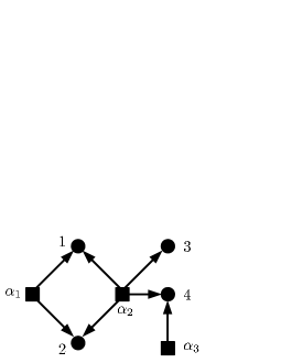
Figure 1: Directed graph representation.

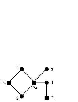
Figure 2: Bipartite graph representation.

Our primary interest is probability density functions that have factorization structures represented by hypergraphs. In such situations, a hypergraph is often referred to as a factor graph and a hyperedge as a factor.

Definition 1

Let $H=(V,F)$ be a hypergraph. For each $i\in V$, let $x_{i}$ be a variable that takes values in a set $\mathcal{X}_{i}$. A probability density function $p$ on $x=(x_{i})_{i\in V}$ is said to be graphically factorized with respect to $H$ if it has the following factorized form

$$p(x)=\frac{1}{Z}\prod_{\alpha\in F}\Psi_{\alpha}(x_{\alpha}),$$ (1)

where $x_{\alpha}=(x_{i})_{i\in\alpha}$, $Z$ is the normalization constant and $\Psi_{\alpha}$ are positive valued functions called compatibility functions. A set of compatibility functions, giving a graphically factorized density function, is called a graphical model. The associated hypergraph $H$ is called the factor graph of the graphical model.

Factor graphs are introduced by Kschischang et al. (2001). Any probability density function on $\mathcal{X}=\prod_{i\in V}\mathcal{X}_{i}$ is trivially graphically factorized with respect to the “one-factor hypergraph”, where the unique factor includes all vertices. It is more informative if the factorization involves factors of small size. Our implicit assumption throughout this paper is that for all factors $\alpha$, $\mathcal{X}_{\alpha}=\prod_{i}\mathcal{X}_{i}$ are small enough, in the sense of cardinality or dimension, to be handled efficiently by computers.

2.2 Loopy Belief Propagation algorithm

Given a graphical model, our task is to solve inference problem such as computation of marginal/conditional density functions and the partition function. Belief Propagation (BP) efficiently computes the exact marginals of a joint distribution that is factorized according to a tree-structured factor graph; Loopy Belief Propagation (LBP) is a heuristic application of the algorithm for factor graphs with cycles, showing successful performance in various problems.

First, in Subsection 2.2.1, we introduce a collection of exponential families called inference family to formulate the LBP algorithm. In order to perform inferences using LBP, we have to fix an inference family that “includes” the given graphical model. Our formulation is a variant of the approach by Wainwright et al. (2003a), where over-complete sufficient statistics are exploited. The detail of the LBP algorithm is described in Subsections 2.2.2.

2.2.1 Exponential families and Inference family

To clarify notations, here we summarize basic facts on exponential families. Let ($\mathcal{X},\mathcal{B},\nu)$ be a measure space. For given $n$ real valued functions (sufficient statistics) ${\phi}(x)=(\phi_{1}(x),\ldots,\phi_{n}(x))$, an exponential family is given by

$$p(x;{\theta})=\exp\left(\sum_{i=1}^{N}\theta_{i}\phi_{i}(x)-\psi({\theta})\right),\qquad\quad\psi({\theta}):=\log\int\exp\left(\sum_{i=1}^{N}\theta_{i}\phi_{i}(x)\right){\rm d}\nu(x).$$

The natural parameter, ${\theta}$, ranges over the set $\Theta:={\rm int}\{{\theta}\in\mathbb{R}^{N};\psi({\theta})<\infty\}$, where int denotes the interior of the set. The function $\psi({\theta})$ is called the log partition function. We always assume that the Hessian of this function (i.e. the covariance matrix) is invertible. The derivative of the log partition function gives a bijective map

$$\Lambda:\Theta\ni\theta\longmapsto\frac{\partial\psi}{\partial\theta}({\theta})={\rm E}_{p_{\boldsymbol{\theta}}}[\boldsymbol{\phi}]\in Y:=\Lambda(\Theta)$$

and this alternative parameter $\eta=\frac{\partial\psi}{\partial\theta}({\theta})$ is called expectation parameter. The inverse of this map is given by the derivative of the Legendre transform $\varphi(\boldsymbol{\eta})=\sup_{\boldsymbol{\theta}\in\Theta}(\sum_{i}\theta_{i}\eta_{i}-\psi(\boldsymbol{\theta}))={\rm E}_{p_{\Lambda^{-1}(\boldsymbol{\eta})}}[\log p_{\Lambda^{-1}(\boldsymbol{\eta})}]$.

Example 1

[Multinomial distributions] Let $\mathcal{X}=\{0,\ldots,N-1\}$ be a finite set with the uniform base measure. One way of taking sufficient statistics is

$$\phi_{k}(x)=\begin{cases}1\text{ \quad if }x=k\\ 0\text{ \quad otherwise}\end{cases}$$ (2)

for $k=0,\ldots,N-2$. Then the given exponential family is called multinomial distributions and coincide with the all probability density functions on $\mathcal{X}$ that has positive probabilities for all elements of $\mathcal{X}$. The region of natural parameters is $\Theta=\mathbb{R}^{N-1}$ and the of expectation parameters is the interior of the probability simplex. That is, $Y=\{(y_{1},\ldots,y_{N});\sum_{k=1}^{N}y_{k}=1,y_{k}>0\}$.

Example 2

[Gaussian distributions] Let $\mathcal{X}=\mathbb{R}^{n}$ with the Lebesgue measure and The exponential family given by the sufficient statistics $\phi(x)=(x_{i},x_{j}x_{k})_{1\leq i\leq n,1\leq j\leq k\leq n}$, is called Gaussian distributions, consists of probability density functions of the form

$$p(\boldsymbol{x};\theta)=\exp\big{(}\sum_{i\leq j}\theta_{ij}x_{i}x_{j}+\sum_{i}\theta_{i}x_{i}-\psi(\theta)\big{)}.$$

Example 3

[Fixed-mean Gaussian distributions] For a given mean vector $\boldsymbol{\mu}=(\mu_{i})$, the fixed-mean Gaussian distributions is the exponential family obtained by the sufficient statistics $\phi(x)=\{(x_{i}-\mu_{i})(x_{j}-\mu_{j})\}_{1\leq i\leq j\leq n}$.

Here and below, we construct a set of exponential families. In order to perform inferences using LBP for a given graphical model, we have to fix a “family” that includes the given probability density function.

Let $H=(V,F)$ be a hypergraph. First, for each vertex $i$, we consider an exponential family $\mathcal{E}_{i}$ with a sufficient statistic $\phi_{i}$ and a base measure $\nu_{i}$ on $\mathcal{X}_{i}$. A natural parameter, expectation parameter, the log partition function and its Legendre transform are denoted by $\theta_{i}$, $\eta_{i}$, $\psi_{i}$ and $\varphi_{i}$ respectively. Secondly, for each factor $\alpha=\{i_{1},\ldots,i_{d_{\alpha}}\}$, we give an exponential family $\mathcal{E}_{\alpha}$ on $\mathcal{X}_{\alpha}=\prod_{i\in\alpha}\mathcal{X}_{i}$ with the base measure $\nu_{\alpha}=\prod_{i\in\alpha}\nu_{i}$ and a sufficient statistic ${{\phi}_{\alpha}}$ of the form

$${{\phi}_{\alpha}}(x_{\alpha})=({{\phi}_{\langle\alpha\rangle}}(x_{\alpha}),\phi_{i_{1}}(x_{i_{1}}),\ldots,\phi_{i_{d_{\alpha}}}(x_{i_{d_{\alpha}}})).$$ (3)

An important point is that ${{\phi}_{\alpha}}$ includes the sufficient statistics for $i\in\alpha$ as its components in addition to ${{\phi}_{\langle\alpha\rangle}}$ indexed by $\alpha\in F$. The natural parameter, expectation parameter, log partition function and its Legendre transform are denoted by

$${{\theta}_{\alpha}}=({{\theta}_{\langle\alpha\rangle}},{\theta}_{\alpha:i_{1}},\ldots,{\theta}_{\alpha:i_{d_{\alpha}}})\in{{\Theta}_{\alpha}},\quad{{\eta}_{\alpha}}=({{\eta}_{\langle\alpha\rangle}},{\eta}_{\alpha:i_{1}},\ldots,{\eta}_{\alpha:i_{d_{\alpha}}})\in{{Y}_{\alpha}},\quad\psi_{\alpha}\text{ and }\varphi_{\alpha}.$$ (4)

The following assumption is indispensable to our analysis:

Assumption 1

For all $i\in V$ and $\alpha\in F$, we assume that the Hessian of the log partition functions , $\psi_{i}$ and $\psi_{\alpha}$, (i.e. the covariance matrix) are invertible in the parameter spaces.

In order to use these exponential families $\mathcal{E}_{\alpha}$ and $\mathcal{E}_{i}$ for LBP, we need another assumption: the family is “closed” under marginalization operation. This type of condition on exponential families is also considered in other litterateurs (Mardia et al., 2009).

Assumption 2 (Marginally closed assumption)

For all pair of $i\in\alpha$,

$$\int p(x_{\alpha}){\rm d}\nu_{\alpha\smallsetminus i}(x_{\alpha\smallsetminus i})\in\mathcal{E}_{i}\quad\text{ for all }p\in\mathcal{E}_{\alpha}.$$ (5)

Definition 2

If a collection of the exponential families $\mathcal{I}:=\{\mathcal{E}_{\alpha},\mathcal{E}_{i}\}$ given by sufficient statistics $({{\phi}_{\langle\alpha\rangle}}(x_{\alpha}),\phi_{i}(x_{i}))_{\alpha\in F,i\in V}$ as above satisfies Assumptions 1 and 2, it is called an inference family associated with a hypergraph $H$. An inference family is called pairwise if the associated hypergraph is a graph.

An inference family has a parameter set $\Theta=\prod_{\alpha}{{\Theta}_{\alpha}}\times\prod_{i}\Theta_{i}$, which is bijectively mapped to the dual parameter set $Y=\prod_{\alpha}{{Y}_{\alpha}}\times\prod_{i}Y_{i}$ by the maps of respective components. An inference family naturally defines an exponential family on $\mathcal{X}=\prod_{i}\mathcal{X}_{i}$ of the sufficient statistic $({{\phi}_{\langle\alpha\rangle}}(x_{\alpha}),\phi_{i}(x_{i}))_{\alpha\in F,i\in V}$. We denote it by $\mathcal{E}(\mathcal{I})$.

Example 4

[Binary pairwise inference family] Consider the case that a graph $G=(V,E)$ is the factor graph. For each $i\in V$, we define an exponential family $\mathcal{E}_{i}$ on $\mathcal{X}_{i}=\{0,1\}$ defined by $\phi_{i}(x_{i})=x_{i}$. For each $\{i,j\}\in E$, we also define multinomial exponential family $\mathcal{E}_{\{i,j\}}$ on $\{0,1\}^{2}$ by $\phi_{\{i,j\}}(x_{i},x_{j})=(x_{i},x_{j},x_{i}x_{j})$, where ${{\phi}_{\langle i,j\rangle}}(x_{i})=x_{i}x_{j}$. Then these exponential family gives an inference family since Assumption 2 is trivially satisfied.

Example 5

[Multinomial inference family] Let $\mathcal{E}_{i}$ be an exponential family of multinomial distributions. Choosing functions ${{\phi}_{\langle\alpha\rangle}}(x_{\alpha})$, we can make the $\mathcal{E}_{\alpha}$ being multinomial distributions on $\mathcal{X}_{\alpha}$; more precisely, we choose ${{\phi}_{\langle\alpha\rangle}}(x_{\alpha})$ so that the components of $\phi_{\alpha}(x_{\alpha})$, which are regarded as $\prod_{i}|\mathcal{X}_{i}|$ dimensional vectors, are linearly independent. Then we obtain an inference family called a multinomial inference family.

Example 6

[Gaussian inference family] We consider the case that $\mathcal{X}_{i}=\mathbb{R}$ . For Gaussian case, given a factor graph $H=(V,F)$, the sufficient statistics are given by

$$\phi_{i}(x_{i})=(x_{i},x_{i}^{2}),\qquad{{\phi}_{\langle\alpha\rangle}}(x_{\alpha})=(x_{i}x_{j})_{i,j\in\alpha,i\neq j}.$$

Then the inference family is called Gaussian inference family. Assumption 2 is satisfied because a marginal of a Gaussian density function is a Gaussian density function. Fixed-mean inference family is analogously defined by $\phi_{i}(x_{i})=(x_{i}-\mu_{i})^{2}$ and ${{\phi}_{\langle\alpha\rangle}}(x_{\alpha})=((x_{i}-\mu_{i})(x_{j}-\mu_{j}))_{i,j\in\alpha,i\neq j}$. Usually, for Gaussian cases, the factor graph $H$ is a graph rather than hypergraphs; thus, we only consider Gaussian inference families on graphs.

2.2.2 LBP algorithm

The LBP algorithm calculates the approximate marginals of a given graphical model $\Psi=\{\Psi_{\alpha}\}$ using the inference family inference family $\mathcal{I}$. We always assume that the inference family includes the given probability density function:

Assumption 3

For every factor $\alpha\in F$, there exists ${{\bar{\theta}}_{\alpha}}$ s.t.

$$\Psi_{\alpha}(x_{\alpha})=\exp\left(\langle{{\bar{\theta}}_{\alpha}},{{\phi}_{\alpha}}(x_{\alpha})\rangle\right).$$ (6)

This is equivalent to the assumption

$$p(x)=\frac{1}{Z}\prod_{\alpha}\Psi_{\alpha}(x_{\alpha})\in\mathcal{E}(\mathcal{I})$$ (7)

up to trivial re-scaling of $\Psi_{\alpha}$, which does not affect LBP algorithm.

The procedures of the LBP algorithm is as follows (Kschischang et al., 2001). For each pair of a vertex $i\in V$ and a factor $\alpha\in F$ satisfying $i\in\alpha$, an initialized message is given in the form of

$$m_{\alpha\rightarrow i}^{0}(x_{i})=\exp(\langle\mu_{\alpha\rightarrow i}^{0},\phi_{i}(x_{i})\rangle),$$ (8)

where the choice of $\mu_{\alpha\rightarrow i}^{0}$ is arbitrary. The set $\{m_{\alpha\rightarrow i}^{0}\}$ or $\{\mu_{\alpha\rightarrow i}^{0}\}$ is called an initialization of the LBP algorithm. At each time $t$, the messages are updated by the following rule:

$$m^{t+1}_{\alpha\rightarrow i}(x_{i})=\omega\int\Psi_{\alpha}(x_{\alpha})\prod_{j\in\alpha,j\neq i}\prod_{\beta\ni j,\beta\neq\alpha}m^{t}_{\beta\rightarrow j}(x_{j})\hskip 2.84526pt{\rm d}\nu_{\alpha\smallsetminus i}({x_{\alpha\smallsetminus i}})\qquad(t\geq 0),$$ (9)

where $\omega$ is a certain scaling constant. See Fig 3 for the illustration of this message update scheme. From Assumptions 2 and 3, the messages keep the form of Eq. (8).

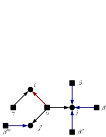
Figure 3: The blue messages contribute to the red message at the next time step.

Since this update rule simultaneously generates all messages of time $t+1$ by those of time $t$, it is called a parallel update. Another possibility of the update is a sequential update, where, at each time step, one message is chosen according to some prescribed or random order of directed edges. In this paper, we mainly discuss the parallel update.

We repeat the update Eq. (9) until the messages converge to a fixed point, though this procedure is not guaranteed to converge. Indeed, it sometimes exhibits oscillatory behaviors. The set of LBP fixed points does not depend on the choices of the update rule, but converging behavior, or dynamics, does depend on the choices.

If the algorithm converges, we obtain the fixed point messages $\{m^{*}_{\alpha\rightarrow i}\}$ and beliefs that are defined by

$$b_{i}(x_{i}):=\omega\prod_{\alpha\ni i}m_{\alpha\rightarrow i}^{*}(x_{i})$$ (10)

$$b_{\alpha}(x_{\alpha}):=\omega\Psi_{\alpha}(x_{\alpha})\prod_{j\in\alpha}\prod_{\beta\ni j,\beta\neq\alpha}m^{*}_{\beta\rightarrow j}(x_{j}),$$ (11)

where $\omega$ denotes (not necessarily the same) normalization constants that require

$$\int b_{i}(x_{i}){\rm d}\nu_{i}=1\quad\text{ and }\quad\int b_{\alpha}(x_{\alpha}){\rm d}\nu_{\alpha}=1.$$ (12)

Note that beliefs automatically satisfy the conditions $b_{\alpha}(x_{\alpha})>0$ and

$$\int b_{\alpha}(x_{\alpha}){\rm d}\nu_{\alpha\smallsetminus i}({x_{\alpha\smallsetminus i}})=b_{i}(x_{i}).$$ (13)

The beliefs are used for approximation of the true marginal density functions.

If $H$ is a tree, the LBP algorithm stops at most $|\vec{E}|$ updates and the computed beliefs are equal to the exact marginals of the given density function.

2.3 Bethe free energy and characterization of LBP fixed points

The Bethe approximation was initiated by Bethe (1935) and was found to be essentially equivalent to LBP by Yedidia et al. (2001). The modern formulation for presenting the approximation is a variational problem of the Bethe free energy (An, 1988). In this subsection, we summarize these facts in our settings.

First, we should introduce the Gibbs free energy function because the Bethe free energy function is a computationally tractable approximation of the Gibbs free energy function. For given graphical model $\Psi=\{\Psi_{\alpha}\}$, the Gibbs free energy $F_{Gibbs}$ is a convex function over the set of probability distributions $\hat{p}$ on $x=(x_{i})_{i\in V}$ defined by

$$F_{Gibbs}(\hat{p})=\int\hat{p}(x)\log\left(\frac{\hat{p}(x)}{\prod_{\alpha}\Psi_{\alpha}(x_{\alpha})}\right){\rm d}\nu(x),$$ (14)

where $\nu=\prod_{i\in V}\nu_{i}$ is the base measure on $\mathcal{X}=\prod_{i\in V}\mathcal{X}_{i}$. Using Kullback-Leibler divergence $D(q||p)=\int\hat{p}\log(q/p)$, Eq. (14) comes to $F_{Gibbs}(\hat{p})=D(\hat{p}||p)-\log Z.$ Therefore, the exact density function Eq. (1) is characterized by a variational problem

$$p(x)=\operatorname*{argmin}_{\hat{p}}F_{Gibbs}(\hat{p}),$$ (15)

where the minimum is taken over all probability distributions on $x$. As suggested from the name of “free energy”, the minimum value of this function is equal to $-\log Z$.

In many cases including discrete variables, computing values of the Gibbs free energy function is intractable in general because the integral in Eq. (14) is indeed a sum over $|\mathcal{X}|=\prod_{i}|\mathcal{X}_{i}|$ states. We introduce functions called Bethe free energy that does not include such an exponential number of state sum.

Definition 3

The Bethe free energy (BFE) function is a function of expectation parameters. For a given inference family $\mathcal{I}$, define $L(\mathcal{I}):=\{\boldsymbol{\eta}=\{{{\eta}_{\alpha}},\eta_{i}\}\in Y|{\eta}_{\alpha:i}=\eta_{i}\ {}^{\forall}(i\in\alpha)\}$ . On this set, the Bethe free energy function is defined by

$$F(\boldsymbol{\eta}):=-\sum_{\alpha\in F}\langle{{\bar{\theta}}_{\alpha}},{{\eta}_{\alpha}}\rangle+\sum_{\alpha\in F}\varphi_{\alpha}({{\eta}_{\alpha}})+\sum_{i\in V}(1-d_{i})\varphi_{i}(\eta_{i}),$$ (16)

where ${{\bar{\theta}}_{\alpha}}$ is the natural parameter of $\Psi_{\alpha}$ in Eq. (6).

An expectation parameter specifies a probability density function in the exponential family. Thus, $\boldsymbol{\eta}\in Y$ specifies $\{b_{\alpha}(x_{\alpha}),b_{i}(x_{i})\}_{\alpha\in F,i\in V}$, where $b_{\alpha}(x_{\alpha})\in\mathcal{E}_{\alpha}$ and $b_{i}(x_{i})\in\mathcal{E}_{i}$. The constraint ${\eta}_{\alpha:i}=\eta_{i}$ means that

$$\int\phi_{i}(x_{i})b_{\alpha}(x_{\alpha}){\rm d}\nu_{\alpha}=\int\phi_{i}(x_{i})b_{i}(x_{i})\nu_{i}.$$

Under Assumption 3, this condition is equivalent to $\int b_{\alpha}(x_{\alpha}){\rm d}\nu_{\alpha\smallsetminus i}=b_{i}(x_{i})$ because a probability density function in $\mathcal{E}_{i}$ is specified by the expectation of $\phi_{i}(x_{i})$. An element of $L$ is called a set of pseudomarginals. Therefore, we have the following identification

$$L=\Big{\{}\{b_{\alpha}(x_{\alpha}),b_{i}(x_{i})\}_{\alpha\in F,i\in V}|~{}b_{\alpha}(x_{\alpha})\in\mathcal{E}_{\alpha},~{}b_{i}(x_{i})\in\mathcal{E}_{i}\quad and\int b_{\alpha}(x_{\alpha}){\rm d}\nu_{\alpha\smallsetminus i}=b_{i}(x_{i})\Big{\}}.$$

The second condition is called local consistency. Under this identification, the Bethe free energy function is

$$F(\{b_{\alpha}(x_{\alpha}),b_{i}(x_{i})\})=-\sum_{\alpha\in{F}}\int b_{\alpha}(x_{\alpha})\log\Psi_{\alpha}(x_{\alpha}){\rm d}\nu_{\alpha} +\sum_{\alpha\in{F}}\int b_{\alpha}(x_{\alpha})\log b_{\alpha}(x_{\alpha}){\rm d}\nu_{\alpha}$$

$$+\sum_{i\in V}(1-d_{i})\int b_{i}(x_{i})\log b_{i}(x_{i}){\rm d}\nu_{i}.$$

If $H$ is a tree, the variational problem of the Bethe free energy over $L$ is equivalent to that of the Gibbs free energy in the following sense. See Wainwright and Jordan (2008) for more details. First, it can be shown that, for any $\{b_{\alpha}(x_{\alpha}),b_{i}(x_{i})\}\in L$,

$$\Pi(\{b_{\alpha}(x_{\alpha}),b_{i}(x_{i})\}):=\prod_{\alpha}b_{\alpha}(x_{\alpha})\prod_{i}b_{i}(x_{i})^{1-d_{i}}$$ (17)

is a probability density function because it is summed up to one. For these type of density functions, we can see that the Gibbs free energy function is equal to the Bethe free energy function: $F=F_{Gibbs}\circ\Pi$. Secondly, it is also known that the true density function $p$ for a tree has the factorization of the form Eq. (17). Therefore, the variational problem Eq. (15) reduces to that of the Bethe free energy function over $L$.

For general factor graphs, the Bethe variational problem approximates the Gibbs variational problem and a minimizer of the Bethe problem can be used to approximate the marginal density function. As shown by Pakzad and Anantharam (2002), the Bethe free energy function is convex if the factor graph has at most one cycle. Therefore, the minimization of the Bethe free energy is easy for these cases. In general, however, the convexity of $F$ is broken as the nullity of the underlying factor graph becomes large, yielding multiple minima. Though the functions $\varphi_{\alpha}$ and $\varphi_{i}$ are convex, the negative coefficients $(1-d_{i})$ makes the function $F$ complex. The positive-definiteness of the Hessian of the Bethe free energy will be analyzed in Section 4 and 5.

The Bethe free energy function gives an alternative description of the LBP fixed points. The following fact is shown by Yedidia et al. (2001); LBP finds a stationary point of the Bethe free energy function, which is a necessary condition of the minimality. We give the proof in our term in Appendix A.2.

Theorem 4

Let $\mathcal{I}$ be an inference family and $\Psi=\{\Psi_{\alpha}\}$ be a graphical model. The following sets are naturally identified each other.

1. The set of fixed points of loopy belief propagation.

2. The set of stationary points of $F$ over $L(\mathcal{I})$.

3 Graph zeta function

The aim of this section is to introduce the graph zeta function and develop some results, which are used in the later sections.

Ihara’s graph zeta function was originally introduced by Y. Ihara (1966) for a certain algebraic object, and was abstracted and extended to be defined on arbitrary finite graphs by J. P. Serre (1980), Sunada (1986) and Bass (1992). The edge zeta function is a multi-variable generalization of Ihara’s graph zeta function, allowing arbitrary scalar weight for each directed edge (Stark and Terras, 1996). Extending those graph zeta functions, we introduce a graph zeta function defined on hypergraphs with matrix weights.

The central result of this section is the Ihara-Bass type determinant formula in Subsection 3.2. This formula plays an important role in deriving the positive definiteness condition in Subsection 3.4. These results are utilized to establish the relations between this zeta function and the LBP algorithm in the next section.

3.1 Definition of the graph zeta function

In the first part of this subsection, we further introduce basic definitions and notations of hypergraphs required for the definition of our graph zeta function.

Let $H=(V,F)$ be a hypergraph. As noted before, it can be regarded as a directed graph $H=(V\cup F,\vec{E})$. For each edge $e=(\alpha\rightarrow i)\in\vec{E}$, $s(e)=\alpha\in F$ is the starting hyperedge of $e$ and $t(e)=i\in V$ is the terminus vertex of $e$. If two edges $e,e^{\prime}\in\vec{E}$ satisfy conditions $t(e)\in s(e^{\prime})$ and $t(e)\neq t(e^{\prime})$, this pair is denoted by $e\rightharpoonup e^{\prime}$. (See Figure 4.) A sequence of directed edges $(e_{1},\ldots,e_{k})$ is said to be a closed geodesic if $e_{l}\rightharpoonup e_{l+1}$ for $l\in\mathbb{Z}/k\mathbb{Z}$. For a closed geodesic $c$, we may form the m-multiple $c^{m}$ by repeating $c$ $m$-times. If $c$ is not a multiple of strictly shorter closed geodesic, $c$ is said to be prime. For example, a closed geodesic $c=(e_{1},e_{2},e_{3},e_{1},e_{2},e_{3})$ is not prime because $c=(e_{1},e_{2},e_{3})^{2}$. A closed geodesic $c=(e_{1},e_{2},e_{3},e_{4},e_{1},e_{2},e_{3})$ is prime because it is not $c\neq c^{\prime m}$ for any $c^{\prime}$ and $m(\geq 2)$. Two closed geodesics are said to be equivalent if one is obtained by cyclic permutation of the other. For example, closed geodesics $(e_{1},e_{2},e_{3}),(e_{2},e_{3},e_{1})\text{ and }(e_{3},e_{1},e_{2})$ are equivalent. An equivalence class of a prime closed geodesic is called a prime cycle. The set of prime cycles of $H$ is denoted by $\mathfrak{P}_{H}$.

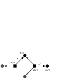
Figure 4: Example of the relation $e\rightharpoonup e^{\prime}$.

If $H$ is a graph (i.e. $d_{\alpha}=2$ for all $\alpha\in F$), these definitions reduce to standard definitions (Kotani and Sunada, 2000). (We will explicitly give them in Subsection 3.3.) In this case, a factor $\alpha=\{i,j\}$ is identified with an undirected edge $ij$ and $(\alpha\rightarrow i)$ is identified with a directed edge $(i\rightarrow j)$.

Usually, in graph theory, Ihara’s graph zeta function is a uni-variate function and associated with a graph. Our graph zeta function is much more involved: it is defined on a hypergraph having weights of matrices. To define matrix weights, we have to prescribe its sizes; we associate a positive integer $r_{e}$ with each edge $e\in\vec{E}$.

Here are additional notations used in the following definition. The set of functions on $\vec{E}$ that take values on $\mathbb{C}^{r_{e}}$ for each $e\in\vec{E}$ is denoted by $\mathfrak{X}(\vec{E})$. The set of $n_{1}\times n_{2}$ complex matrices is denoted by ${\rm M}(n_{1},n_{2})$.

Definition 5

Assume that for each $e^{\prime}\rightharpoonup e$, a matrix weight $u_{e^{\prime}\rightharpoonup e}\in{\rm M}(r_{e},r_{e^{\prime}})$ is associated. For this matrix weights $\boldsymbol{u}=\{u_{e^{\prime}\rightharpoonup e}\}$, the graph zeta function of $H$ is defined by

$$\zeta_{H}(\boldsymbol{u}):=\prod_{\mathfrak{p}\in\mathfrak{P}_{H}}\frac{1}{\det\big{(}I-\pi(\mathfrak{p})\big{)}},$$

where $\pi(\mathfrak{p}):=$ $u_{e_{k}\rightharpoonup e_{1}}\ldots u_{e_{2}\rightharpoonup e_{3}}u_{e_{1}\rightharpoonup e_{2}}$ for $\mathfrak{p}=(e_{1},\ldots,e_{k})$.

Since $\det(I_{n}-AB)=\det(I_{m}-BA)$ for $n\times m$ and $m\times n$ matrices $A$ and $B$, $\det(I-\pi(\mathfrak{p}))$ is well defined for an equivalence class $\mathfrak{p}$. The definition is an analogue of the Euler product formula of the Riemann zeta function which is represented by the product over all the prime numbers.

If $H$ is a graph and $r_{e}=1$ for all $e\in\vec{E}$, this zeta function reduces to the edge zeta function by Stark and Terras (1996). If in addition all these scalar weights are set to be equal, i.e. $u_{e^{\prime}\rightharpoonup e}=u$, the zeta function reduces to the Ihara zeta function. These reductions will be discussed in Subsection 3.3. Moreover, for general hypergraphs, we obtain the one-variable hypergraph zeta function by setting all matrix weights to be the same scalar $u$ (Storm, 2006).

Example 7

$\zeta_{H}(\boldsymbol{u})=1$ if $H$ is a tree. For 1-cycle graph $C_{N}$ of length $N$, the prime cycles are $(e_{1},e_{2},\ldots,e_{N})$ and $(\bar{e}_{N},\bar{e}_{N-1},\ldots,\bar{e}_{1})$. (See Figure 5.) The zeta function is

$$\zeta_{C_{N}}(\boldsymbol{u})=\det(I_{r_{e_{1}}}-u_{e_{N}\rightharpoonup e_{1}}\ldots u_{e_{2}\rightharpoonup e_{3}}u_{e_{1}\rightharpoonup e_{2}})^{-1}\det(I_{r_{\bar{e}_{N}}}-u_{\bar{e}_{1}\rightharpoonup\bar{e}_{N}}\ldots u_{\bar{e}_{N-1}\rightharpoonup\bar{e}_{N-2}}u_{\bar{e}_{N}\rightharpoonup\bar{e}_{N-1}})^{-1}.$$

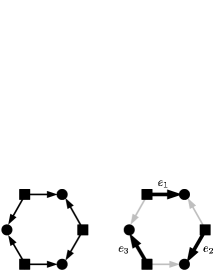
Figure 5: $C_{3}$ and its prime cycles.

Except for the above two types of hypergraphs, the number of prime cycles is infinite. Therefore, rigorously speaking, we have to care about the convergence of the product and restrict the definition for sufficiently small matrix weights $\boldsymbol{u}$. However, as we will see below, the zeta function has a determinant formula and is well defined on the whole space of matrix weights. The proof is given in Appendix A.2.

Theorem 6 (The first determinant formula of zeta function)

We define a linear operator $\mathcal{M}(\boldsymbol{u}):\mathfrak{X}(\vec{E})\rightarrow\mathfrak{X}(\vec{E})$ by

$$\mathcal{M}(\boldsymbol{u})f(e)=\sum_{e^{\prime}:e^{\prime}\rightharpoonup e}u_{e^{\prime}\rightharpoonup e}f(e^{\prime})\qquad f\in\mathfrak{X}(\vec{E}).$$

Then, the following formula holds

$$\zeta_{G}(\boldsymbol{u})^{-1}=\det(I-\mathcal{M}(\boldsymbol{u})).$$

This type of determinant formula is well known in the context of graph zeta functions; in fact this theorem is a straightforward generalization of Theorem 3 of Stark and Terras (1996). In the next section we derive a new determinant formula of the zeta function by manipulating the matrix $\mathcal{M}(\boldsymbol{u})$ in the above determinant.

Note that the matrix representation of the operator $\mathcal{M}(\boldsymbol{u})$ is

$$\mathcal{M}(\boldsymbol{u})_{e,e^{\prime}}=\begin{cases}u_{e^{\prime}\rightharpoonup e}\qquad\text{if }e^{\prime}\rightharpoonup e\\ 0\qquad\qquad\text{otherwise.}\end{cases}$$

The simplification of this matrix obtained by setting $r_{e}=1$ and $u=1$ is called directed edge matrix and denoted by $\mathcal{M}$ (Stark and Terras, 1996). Kotani and Sunada (2000) call this matrix a Perron-Frobenius operator. A noteworthy difference, in our and their definitions, is that directions of edges are opposite, because we choose the directions to be consistent with illustrations of the LBP algorithm.

3.2 Determinant formula of Ihara-Bass type

In the previous subsection, we have shown that the zeta function is expressed as a determinant of size $\sum_{e\in\vec{E}}r_{e}$. In this subsection, we show another determinant expression with additional assumptions on the matrix weights. The formula is called Ihara-Bass type determinant formula and plays a key role in proofs of Theorem 10 and Theorem 11.

In the rest of this subsection, we fix a set of positive integers $\{r_{i}\}_{i\in V}$ associated with vertices. Let $\{u^{\alpha}_{i\rightarrow j}\}_{\alpha\in F,i,j\in\alpha}$ be a set of matrices $u^{\alpha}_{i\rightarrow j}\in{\rm M}(r_{j},r_{i},$). Our additional assumption on the set of matrix weights, which is the argument of the zeta function, is that

$$r_{e}:=r_{t(e)}\text{~{} and ~{}}u_{e^{\prime}\rightharpoonup e}:=u^{s(e)}_{t(e^{\prime})\rightarrow t(e)}.$$

Then the graph zeta function can be seen as a function of $\boldsymbol{u}=\{u^{\alpha}_{i\rightarrow j}\}$. With slight abuse of notation, it is also denoted by $\zeta_{H}(\boldsymbol{u})$. Later in Section 4, $r_{i}$ corresponds to the dimension of the sufficient statistic $\phi_{i}$, and $u^{\alpha}_{i\rightarrow j}$ to a matrix ${\rm Var}_{b_{j}}[\phi_{j}]^{-1}{\rm Cov}_{b_{\alpha}}[\phi_{j},\phi_{i}]$.

To state the Ihara-Bass type determinant formula, we introduce a linear operator $\boldsymbol{\iota}(\boldsymbol{u}):\mathfrak{X}(\vec{E})\rightarrow\mathfrak{X}(\vec{E})$ defined by

$$(\boldsymbol{\iota}(\boldsymbol{u})f)(e):=\sum_{e^{\prime}:{s(e^{\prime})=s(e)\atop t(e^{\prime})\neq t(e)}}u^{s(e)}_{t(e^{\prime})\rightarrow t(e)}f(e^{\prime})\qquad f\in\mathfrak{X}(\vec{E}).$$

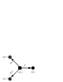
Figure 6: Illustration for the definition of $\boldsymbol{\iota}(\boldsymbol{u})$.

The matrix representation of $\boldsymbol{\iota}(\boldsymbol{u})$ is a block diagonal matrix because it acts on each factor separately. Therefore $I+\boldsymbol{\iota}(\boldsymbol{u})$ is also a block diagonal matrix. Each block is indexed by $\alpha\in F$ and denoted by $U_{\alpha}$. Thus, for $\alpha=\{i_{1},\ldots,i_{d_{\alpha}}\}$,

$$U_{\alpha}=\begin{bmatrix}I_{r_{i_{1}}}&u^{\alpha}_{i_{2}\rightarrow i_{1}}&\cdots&u^{\alpha}_{i_{d_{\alpha}}\rightarrow i_{1}}\\ u^{\alpha}_{i_{1}\rightarrow i_{2}}&I_{r_{i_{2}}}&\cdots&u^{\alpha}_{i_{d_{\alpha}}\rightarrow i_{2}}\\ \vdots&\vdots&\ddots&\vdots\\ u^{\alpha}_{i_{d_{1}\rightarrow i_{d_{\alpha}}}}&u^{\alpha}_{i_{d_{2}\rightarrow i_{d_{\alpha}}}}&\cdots&I_{r_{i_{d_{\alpha}}}}\\ \end{bmatrix}.$$ (18)

We also define $w^{\alpha}_{i\rightarrow j}$ by the elements of $W_{\alpha}=U_{\alpha}^{-1}$:

$$W_{\alpha}=\begin{bmatrix}w^{\alpha}_{i_{1}\rightarrow i_{1}}&w^{\alpha}_{i_{2}\rightarrow i_{1}}&\cdots&w^{\alpha}_{i_{d_{\alpha}}\rightarrow i_{1}}\\ w^{\alpha}_{i_{1}\rightarrow i_{2}}&w^{\alpha}_{i_{2}\rightarrow i_{2}}&\cdots&w^{\alpha}_{i_{d_{\alpha}}\rightarrow i_{2}}\\ \vdots&\vdots&\ddots&\vdots\\ w^{\alpha}_{i_{d_{1}\rightarrow i_{d_{\alpha}}}}&w^{\alpha}_{i_{d_{2}\rightarrow i_{d_{\alpha}}}}&\cdots&w^{\alpha}_{i_{d_{\alpha}}\rightarrow i_{d_{\alpha}}}\\ \end{bmatrix}.$$ (19)

Similar to the definition of $\mathfrak{X}(\vec{E})$ in Subsection 3.1, we define $\mathfrak{X}(V)$ as the set of functions on $V$ that takes value on $\mathbb{C}^{r_{i}}$ for each $i\in V$.

Theorem 7 (Determinant formula of Ihara-Bass type)

Let $\mathcal{D}$ be $\mathcal{W}$ are linear transforms on $\mathfrak{X}(V)$ defined by

$$(\mathcal{D}g)(i):=d_{i}g(i),\qquad(\mathcal{W}g)(i):=\sum_{{e,e^{\prime}\in\vec{E}\atop{t(e)=i,s(e)=s(e^{\prime})}}}w^{s(e)}_{t(e^{\prime})\rightarrow i}g(t(e^{\prime})).$$ (20)

Then, we have the following formula

$$\zeta_{G}(\boldsymbol{u})^{-1}=\det\big{(}I_{r_{V}}-\mathcal{D}+\mathcal{W}\big{)}\prod_{\alpha\in F}\det U_{\alpha},$$

where $r_{V}:=\sum_{i\in V}r_{i}$

The proof is given in Appendix A.2

3.3 Ihara-Bass type determinant formula on ordinary graphs

In this subsection, we explicitly write definitions and the above formula for better understanding. A hypergraph $H=(V,F)$, which has only hyperedges of degrees two, is naturally identified with an (undirected) graph $G_{H}=(V,E)$. In the next section, we see that this case corresponds to the pairwise inference family.

First, we define the zeta function $Z_{G}$ of a graph $G=(V,E)$. For each undirected edge, we make a pair of oppositely directed edges, which form a set of directed edges $\vec{E}$. Thus $|\vec{E}|=2|E|$. For each directed edge $e\in\vec{E}$, $o(e)\in V$ is the origin of $e$ and $t(e)\in V$ is the terminus of $e$. For $e\in\vec{E}$, the inverse edge is denoted by $\bar{e}$, and the corresponding undirected edge by $[e]=[\bar{e}]\in E$.

A closed geodesic in $G$ is a sequence $(e_{1},\ldots,e_{k})$ of directed edges such that $t(e_{i})=o(e_{i+1}),e_{i}\neq\bar{e}_{i+1}$ for $i\in\mathbb{Z}/k\mathbb{Z}$. Prime cycles are defined in the same manner to that of hypergraphs. The set of prime cycles is denoted by $\mathfrak{P}_{G}$.

Definition 8

Let $G=(V,E)$ a graph. For given positive integers $\{r_{i}\}_{i\in V}$ and matrix weights $\boldsymbol{u}=\{u_{e}\}_{e\in\vec{E}}$ with $u_{e}\in{\rm M}(r_{t(e)},r_{o(e)})$,

$$Z_{G}(\boldsymbol{u}):=\prod_{\mathfrak{p}\in\mathfrak{P}_{G}}\det(1-\pi(\mathfrak{p}))^{-1},\quad\pi(\mathfrak{p}):=u_{e_{1}}\cdots u_{e_{k}}\quad\text{ for }\mathfrak{p}=(e_{1},\ldots,e_{k}).$$

Since $\mathfrak{P}_{{\rm G}_{H}}$ is naturally identified with $\mathfrak{P}_{H}$, $Z_{{\rm G}_{H}}=\zeta_{H}$ holds. This zeta function is the matrix weight extension of the edge zeta function analyzed by Stark and Terras (1996).

Since the degree of every hyperedge is equal to two for a graph, the matrix $W_{\alpha}$ defined in Eq. (19) has explicit expressions. Using this fact, we obtain the following simplification of Theorem 7.

Corollary 9

For a graph $G=(V,E)$,

$$Z_{G}(\boldsymbol{u})^{-1}=\det(I+\hat{\mathcal{D}}(\boldsymbol{u})-\hat{\mathcal{A}}(\boldsymbol{u}))\prod_{[e]\in{E}}\det(I-u_{e}u_{\bar{e}}),$$ (21)

where $\hat{\mathcal{D}}$ and $\hat{\mathcal{A}}$ are defined by

$$(\hat{\mathcal{D}}(\boldsymbol{u})g)(i):=\Big{(}\sum_{e:t(e)=i}(I_{r_{i}}-u_{e}u_{\bar{e}})^{-1}u_{e}u_{\bar{e}}\Big{)}g(i),$$ (22)

$$(\hat{\mathcal{A}}(\boldsymbol{u})g)(i):=\sum_{e:t(e)=i}(I_{r_{i}}-u_{e}u_{\bar{e}})^{-1}u_{e}g(o(e)).$$ (23)

Proof  For $e=(i\rightarrow j)$, the $U_{[e]}$ block is given by

$$U_{[e]}=\begin{bmatrix}I_{r_{i}}&u_{e}\\ u_{\bar{e}}&I_{r_{j}}\\ \end{bmatrix}$$

Therefore $\det U_{[e]}=\det(I_{r_{i}}-u_{e}u_{\bar{e}})$ and the inverse $W_{[e]}$ is

$$W_{[e]}=\begin{bmatrix}(I_{r_{i}}-u_{e}u_{\bar{e}})^{-1}&0\\ 0&(I_{r_{j}}-u_{\bar{e}}u_{e})^{-1}\\ \end{bmatrix}\begin{bmatrix}I_{r_{i}}&-u_{e}\\ -u_{\bar{e}}&I_{r_{j}}\\ \end{bmatrix}.$$

Plugging these equations into Theorem 7, we obtain the assertion.  

Mizuno and Sato (2004); Horton et al. (2008) have derived a weighted graph version of Ihara-Bass type determinant formula under assumption that the scalar weights $\{u_{e}\}$ satisfy conditions $u_{e}u_{\bar{e}}=u^{2}$. In this case, the factors $(1-u_{e}u_{\bar{e}})^{-1}$ in Eqs. (22,23) do not depend on $e$ and Eq. (21) is further simplified. Corollary 9 gives the extension of the result to graphs with arbitrary weights. A direct proof of Corollary 9, without discussing hypergraphs, is found in the supplementary material of Watanabe and Fukumizu (2009).

If all the weights are set to $u$, the result reduces to the following formula known as Ihara-Bass formula:

$$Z_{G}(u)^{-1}=(1-u^{2})^{|E|-|V|}\det(I-u\mathcal{A}+u^{2}(\mathcal{D}-I)),$$

where $\mathcal{D}$ is the degree matrix defined by $\mathcal{D}_{i,j}=d_{i}\delta_{i,j}$, and $\mathcal{A}$ is the adjacency matrix by

$$\mathcal{A}_{i,j}=\begin{cases}1&\quad\text{if}\quad\{i,j\}\in E\\ 0&\quad\text{otherwise.}\end{cases}$$

Many authors have discussed the proof of the Ihara-Bass formula. The first proof was given by Bass (1992). See Kotani and Sunada (2000); Stark and Terras (1996) for others. A combinatorial proof is given by Foata and Zeilberger (1999).

3.4 Positive definiteness condition

The Ihara-Bass type determinant formula relates the matrices $\mathcal{M}(\boldsymbol{u})$ and $(I_{r_{V}}-\mathcal{D}+\mathcal{W})$. In the later sections, we see that $\mathcal{M}(\boldsymbol{u})$ corresponds to the derivative of the LBP update and $(I_{r_{V}}-\mathcal{D}+\mathcal{W})$ is closely related to the Hessian of the Bethe free energy function.

The following theorem is fundamental to prove Theorem 14.

Theorem 10

Assume that $\boldsymbol{u}=\{u^{\alpha}_{i\rightarrow j}\}_{\alpha\in F,i,j\in\alpha}$ satisfies $u^{\alpha}_{i\rightarrow j}=u^{\alpha}_{j\rightarrow i}$ and $\|u^{\alpha}_{i\rightarrow j}\|<1$, where $\|\cdot\|$ is an arbitrary operator norm. If ${\rm Spec}(\mathcal{M}(\boldsymbol{u}))\hskip 1.42262pt\subset\hskip 1.42262pt\mathbb{C}\smallsetminus\mathbb{R}_{\geq 1}$, where ${\rm Spec}(\cdot)$ denotes the set of eigenvalues, then $(I_{r_{V}}-\mathcal{D}+\mathcal{W})$ is a positive definite matrix.

Proof  From the assumption of symmetry, $W_{\alpha}$ in Eq. (19) is a symmetric matrix. Therefore, $\mathcal{W}$, defined in Eq. (20), is also symmetric. To prove the positive definiteness, we define $u^{\alpha}_{i\rightarrow j}(t):=tu^{\alpha}_{i\rightarrow j}\quad(t\in[0,1])$, which implies $\mathcal{M}(\boldsymbol{u}(t))=t\mathcal{M}(\boldsymbol{u})$. From the assumption, $U_{\alpha}(t)$ is invertible and thus $W_{\alpha}(t)$ is well defined for all $t$. If $t=0$, $W_{\alpha}(0)=\mathcal{D}$ and $I-\mathcal{D}+\mathcal{W}(0)=I$ is obviously positive definite. Since the eigenvalues of a symmetric matrix are real and continuous with respect to its entries, it is enough to prove that $\det(I-\mathcal{D}+\mathcal{W}(t))\neq 0$ on the interval $[0,1]$. Under the condition on the eigenvalues of $\mathcal{M}(\boldsymbol{u})$, $\det(I-\mathcal{M}(\boldsymbol{u}(t)))\neq 0$ holds for $t\in[0,1]$. Therefore, Theorem 7 implies the claim.  

4 Main theoretical results

In this section, we establish the connection between the graph zeta function and the Bethe free energy function. These results form a basis of the analyses in later sections.

In Subsection 4.1, we prove a formula using the Ihara-Bass type determinant formula proved in the previous section. The formula shows a concrete relation between the Bethe free energy function and the graph zeta function. In Subsection 4.2, we give a condition that the Hessian of the Bethe free energy function is positive-definite.

4.1 Bethe-zeta formula

In this subsection, we show that the determinant of the Hessian of the Bethe free energy function is essentially equal to the reciprocal of the graph zeta function.

In order to make the assertion clear, we first recall the definitions and notations. Let $H=(V,F)$ be a hypergraph and let $\mathcal{I}=\{\mathcal{E}_{\alpha},\mathcal{E}_{i}\}$ be an inference family on $H$. Exponential families $\mathcal{E}_{i}$ and $\mathcal{E}_{\alpha}$ are given by sufficient statistics $\phi_{i}$ and ${{\phi}_{\alpha}}$ as discussed in Subsection 2.2.1. Furthermore, as discussed in Subsection 2.3, a point $\boldsymbol{\eta}=\{{{\eta}_{\langle\alpha\rangle}},\eta_{i}\}\in L$ is identified with a set of pseudomarginals $\{b_{\alpha}(x_{\alpha}),b_{i}(x_{i})\}_{\alpha\in F,i\in V}$.

Theorem 11

At any point of $\boldsymbol{\eta}=\{{{\eta}_{\langle\alpha\rangle}},\eta_{i}\}\in L$ the following equality holds.

$$\zeta_{H}(\boldsymbol{u})^{-1}=\det(I-\mathcal{M}(\boldsymbol{u}))=\det(\nabla^{2}F)\prod_{\alpha\in F}\det({\rm Var}_{b_{\alpha}}[{{\phi}_{\alpha}}])\prod_{i\in V}\det({\rm Var}_{b_{i}}[\phi_{i}])^{1-d_{i}},$$

where

$$u^{\alpha}_{i\rightarrow j}:={\rm Var}_{b_{j}}[{\phi}_{j}]^{-1}{\rm Cov}_{b_{\alpha}}[{\phi}_{j},{\phi}_{i}]$$ (24)

is an $r_{j}\times r_{i}$ matrix, and $\nabla^{2}F$ is the Hessian matrix with respect to the coordinate $\{{{\eta}_{\langle\alpha\rangle}},\eta_{i}\}$.

Note that he Hessian $\nabla^{2}F$ does not depend on the given compatibility functions $\Psi_{\alpha}$ because those only affect linear terms in $F$, and thus the formula is a property of inference family $\mathcal{I}$. Note also that the determinants of variances in the formula are always positive, because we assume all the local exponential families $\mathcal{E}_{\alpha}$ and $\mathcal{E}_{i}$ have positive definite covariance matrices.

The proof is based on the Ihara-Bass type determinant formula; we check that the Hessian $\nabla^{2}F$ is related to the matrix $(I-\mathcal{D}+\mathcal{W})$ if weights has the form of Eq. (24). The key condition satisfied on the set $L$ is ${\rm Var}_{b_{\alpha}}[\phi_{i}]={\rm Var}_{b_{i}}[\phi_{i}]$.

Proof  From the definition of the Bethe free energy function Eq. (16), the (V,V)- block of $\nabla^{2}F$ is given by

$$\frac{\partial^{2}F}{\partial\eta_{i}\partial\eta_{i}}=\sum_{\alpha\ni i}\frac{\partial^{2}\varphi_{\alpha}}{\partial\eta_{i}\partial\eta_{i}}+(1-d_{i})\frac{\partial^{2}\varphi_{i}}{\partial\eta_{i}\partial\eta_{i}},\quad\frac{\partial^{2}F}{\partial\eta_{i}\partial\eta_{j}}=\sum_{\alpha\supset\{i,j\}}\frac{\partial^{2}\varphi_{\alpha}}{\partial\eta_{i}\partial\eta_{j}}\quad(i\neq j).$$

The (V,F)-block and (F,F)-block are given by

$$\frac{\partial^{2}F}{\partial\eta_{i}\partial{{\eta}_{\langle\alpha\rangle}}}=\frac{\partial^{2}\varphi_{\alpha}}{\partial\eta_{i}\partial{{\eta}_{\langle\alpha\rangle}}},\quad\quad\frac{\partial^{2}F}{\partial{{\eta}_{\langle\alpha\rangle}}\partial{{\eta}_{\langle\beta\rangle}}}=\frac{\partial^{2}\varphi_{\alpha}}{\partial{{\eta}_{\langle\alpha\rangle}}\partial{{\eta}_{\langle\beta\rangle}}}\delta_{\alpha,\beta}.$$

Using the diagonal blocks of (F,F)-block, we erase (V,F)-block and (F,V)-block of the Hessian by Gaussian elimination. In other words, we choose a square matrix $X$ such that $\det X=1$ and

$$X^{T}(\nabla^{2}F)X=\begin{bmatrix}\quad Y&0\\ \quad 0&\Big{(}\frac{\partial^{2}F}{\partial{{\eta}_{\langle\alpha\rangle}}\partial{{\eta}_{\langle\beta\rangle}}}\Big{)}\end{bmatrix},$$

in which

$$Y_{i,i} =\sum_{\alpha\ni i}\left\{\frac{\partial^{2}\varphi_{\alpha}}{\partial\eta_{i}\partial\eta_{i}}-\frac{\partial^{2}\varphi_{\alpha}}{\partial\eta_{i}\partial{{\eta}_{\langle\alpha\rangle}}}\left(\frac{\partial^{2}\varphi_{\alpha}}{\partial{{\eta}_{\langle\alpha\rangle}}\partial{{\eta}_{\langle\alpha\rangle}}}\right)^{-1}\frac{\partial^{2}\varphi_{\alpha}}{\partial{{\eta}_{\langle\alpha\rangle}}\partial\eta_{i}}\right\}+(1-d_{i})\frac{\partial^{2}\varphi_{i}}{\partial\eta_{i}\partial\eta_{i}},$$ (25)

$$Y_{i,j} =\sum_{\alpha\supset\{i,j\}}\left\{\frac{\partial^{2}\varphi_{\alpha}}{\partial\eta_{i}\partial\eta_{j}}-\frac{\partial^{2}\varphi_{\alpha}}{\partial\eta_{i}\partial{{\eta}_{\langle\alpha\rangle}}}\left(\frac{\partial^{2}\varphi_{\alpha}}{\partial{{\eta}_{\langle\alpha\rangle}}\partial{{\eta}_{\langle\alpha\rangle}}}\right)^{-1}\frac{\partial^{2}\varphi_{\alpha}}{\partial{{\eta}_{\langle\alpha\rangle}}\partial\eta_{j}}\right\}.$$ (26)

On the other hand, since $u^{\alpha}_{i\rightarrow j}:=$ ${\rm Var}_{b_{j}}[{\phi}_{j}]^{-1}$ ${\rm Cov}_{b_{\alpha}}[{\phi}_{j},{\phi}_{i}]$, the matrix $U_{\alpha}$ defined in Eq. (18) is

$$U_{\alpha}={\rm diag}({\rm Var}[\phi_{i}]^{-1}|i\in\alpha)\hskip 2.84526pt{\rm Var}_{b_{\alpha}}[(\phi_{i})_{i\in\alpha}].$$ (27)

Since the matrix ${\rm Var}_{b_{\alpha}}[(\phi_{i})_{i\in\alpha}]$ is a submatrix of ${\rm Var}_{b_{\alpha}}[{{\phi}_{\alpha}}]$, its inverse can be expressed by submatrices of ${\rm Var}_{b_{\alpha}}[{{\phi}_{\alpha}}]^{-1}=\frac{\partial^{2}\varphi_{\alpha}}{\partial{{\eta}_{\alpha}}\partial{{\eta}_{\alpha}}}$ using the Schur complement formula, which shows that the elements of $W_{\alpha}=U_{\alpha}^{-1}$ is given by

$$w^{\alpha}_{j\rightarrow i}=\left\{\frac{\partial^{2}\varphi_{\alpha}}{\partial\eta_{i}\partial\eta_{j}}-\frac{\partial^{2}\varphi_{\alpha}}{\partial\eta_{i}\partial{{\eta}_{\langle\alpha\rangle}}}\left(\frac{\partial^{2}\varphi_{\alpha}}{\partial{{\eta}_{\langle\alpha\rangle}}\partial{{\eta}_{\langle\alpha\rangle}}}\right)^{-1}\frac{\partial^{2}\varphi_{\alpha}}{\partial{{\eta}_{\langle\alpha\rangle}}\partial\eta_{j}}\right\}{\rm Var}[\phi_{j}].$$ (28)

It follows from Eq. (25),(26) and (28) that

$$Y\hskip 2.84526pt{\rm diag}\left({\rm Var}[\phi_{i}]|i\in V\right)=I-\mathcal{D}+\mathcal{W},$$

where $\mathcal{D}$ and $\mathcal{W}$ are defined in Eq. (20). Accordingly, we obtain

$$\zeta_{H}(\boldsymbol{u})^{-1} =\det(I-\mathcal{D}+\mathcal{W})\prod_{\alpha\in F}\det U_{\alpha}$$

$$=\det Y\prod_{i\in V}\det({\rm Var}[\phi_{i}])\prod_{\alpha\in F}\frac{\det\left({\rm Var}_{b_{\alpha}}[(\phi_{i})_{i\in\alpha}]\right)}{\prod_{j\in\alpha}\det\left({\rm Var}[\phi_{j}]\right)}$$

$$=\det\left(\nabla^{2}F\right)\prod_{i\in V}\det({\rm Var}[\phi_{i}])^{1-d_{i}}\prod_{\alpha\in F}\frac{\det\left({\rm Var}_{b_{\alpha}}[(\phi_{i})_{i\in\alpha}]\right)}{\det\left(\frac{\partial^{2}\varphi_{\alpha}}{\partial{{\eta}_{\langle\alpha\rangle}}\partial{{\eta}_{\langle\alpha\rangle}}}\right)}$$

$$=\det\left(\nabla^{2}F\right)\prod_{\alpha\in F}\det({\rm Var}_{b_{\alpha}}[{{\phi}_{\alpha}}])\prod_{i\in V}\det({\rm Var}_{b_{i}}[{\phi}_{i}])^{1-d_{i}},$$

where $\det\left({\rm Var}_{b_{\alpha}}[(\phi_{i})_{i\in\alpha}]\right)\det\left(\frac{\partial^{2}\varphi_{\alpha}}{\partial{{\eta}_{\langle\alpha\rangle}}\partial{{\eta}_{\langle\alpha\rangle}}}\right)^{-1}$ $=\det\left({\rm Var}[{{\phi}_{\alpha}}]\right)$ is used.  

In the rest of this subsection, we rewrite the Bethe-zeta formula in some specific cases. Especially, we give explicit expressions of the determinants of the variance matrices.

Case 1: Multinomial inference family

First, we consider the multinomial case. If we take the sufficient statistics of multinomial exponential family as in Example 1, the determinant of the variance is

$$\det\left({\rm Var}_{p}[{\phi}]\right)=\prod_{k=1}^{N}p(k).$$

Therefore, the theorem reduces to the following form .

Corollary 12 (Bethe-zeta formula for multinomial inference family)

For any $\{b_{\alpha}(x_{\alpha}),b_{i}(x_{i})\}\in L$ the following equality holds.

$$\zeta_{G}(\boldsymbol{u})^{-1}=\det(\nabla^{2}F)\prod_{\alpha\in F}\prod_{x_{\alpha}}b_{\alpha}(x_{\alpha})\prod_{i\in V}\prod_{x_{i}}b_{i}(x_{i})^{1-d_{i}},$$

where $u^{\alpha}_{i\rightarrow j}:=$ ${\rm Var}_{b_{j}}[{\phi}_{j}]^{-1}$ ${\rm Cov}_{b_{\alpha}}[{\phi}_{j},{\phi}_{i}]$ is an $(N_{j}-1)\times(N_{i}-1)$ matrix.

For binary and pairwise case, this formula is first shown by Watanabe and Fukumizu (2009).

Case 2: Fixed-mean Gaussian inference family

Let $G=(V,E)$ be a graph. We consider the fixed-mean Gaussian inference family on $G$. For a given vector $\boldsymbol{\mu}=(\mu_{i})_{i\in V}$, the inference family is constructed from sufficient statistics $\phi_{i}(x_{i})=(x_{i}-\mu_{i})^{2}\quad\text{ and }\quad{{\phi}_{\langle i,j\rangle}}(x_{i},x_{j})=(x_{i}-\mu_{i})(x_{j}-\mu_{j}).$ Their expectation parameters are denoted by $\eta_{ii}$ and $\eta_{ij}$, respectively. The variances and covariances are

$${\rm Var}[\phi_{i}]=2\eta_{ii}^{2},\quad{\rm Var}[\phi_{\{i,j\}}]=\small\begin{bmatrix}2\eta_{ii}^{2}&2\eta_{ij}^{2}&2\eta_{ii}\eta_{ij}\\ 2\eta_{ij}^{2}&2\eta_{jj}^{2}&2\eta_{jj}\eta_{ij}\\ 2\eta_{ii}\eta_{ij}&2\eta_{jj}\eta_{ij}&\eta_{ij}^{2}+\eta_{ii}\eta_{jj}\\ \end{bmatrix},$$

where $\phi_{\{i,j\}}(x_{i},x_{j})=\left((x_{i}-\mu_{i})^{2},(x_{j}-\mu_{j})^{2},(x_{i}-\mu_{i})(x_{j}-\mu_{j})\right).$ Therefore, $\det({\rm Var}[\phi_{\{i,j\}}])=4(\eta_{ii}\eta_{jj}-\eta_{ij}^{2})^{3}$.

Corollary 13

[Bethe-zeta formula for fixed-mean Gaussian inference family ] For any $\{\eta_{ii},\eta_{ij}\}\in L$ the following equality holds.

$$Z_{G}(\boldsymbol{u})^{-1}=\det(\nabla^{2}F)\prod_{i\in V}\eta_{ii}^{2(1-d_{i})}\prod_{ij\in E}(\eta_{ii}\eta_{jj}-\eta_{ij}^{2})^{3}\hskip 5.69054pt2^{|V|,}$$

where $u_{i\rightarrow j}:=\eta_{ij}^{2}\eta_{jj}^{-2}$ is a scalar value.

One interesting point of this case is that the edge weights $u_{i\rightarrow j}$ are always positive.

4.2 Positive definiteness condition

In this section, we derive a condition that guarantees the positive-definiteness of the Hessian of the Bethe free energy function. It is based on Theorem 10, which gives a condition that the matrix $(I-\mathcal{D}+\mathcal{W})$ is positive definite in terms of the matrix $\mathcal{M}(\boldsymbol{u})$. As we have seen in the proof of the previous theorem, $\nabla^{2}F$ and $(I-\mathcal{D}+\mathcal{W})$ are essentially the same. Thus, we obtain the following theorem.

Theorem 14

Let $\boldsymbol{u}$ be given by $\boldsymbol{\eta}\in L$ using Eq. (24). Then,

$${\rm Spec}(\mathcal{M}(\boldsymbol{u}))\hskip 1.42262pt\subset\hskip 1.42262pt\mathbb{C}\smallsetminus\mathbb{R}_{\geq 1}\quad\Longrightarrow\quad\nabla^{2}F(\boldsymbol{\eta})\text{ is a positive definite matrix.}$$

Before the proof of the theorem, we remark the following fact. It implies that we can change the matrix weight to the correlation coefficient matrices.

Lemma 15

Let $\boldsymbol{\eta}$ be a point in $L$, $u^{\alpha}_{i\rightarrow j}$ be given by Eq. (24), and

$$c^{\alpha}_{i\rightarrow j}:={\rm Cor}_{b_{\alpha}}[\phi_{j},\phi_{i}]={\rm Var}_{b_{\alpha}}[\phi_{j}]^{-1/2}{\rm Cov}_{b_{\alpha}}[\phi_{j},\phi_{i}]{\rm Var}_{b_{\alpha}}[\phi_{i}]^{-1/2}$$

be the correlation coefficient matrix, where $b_{\alpha}$ corresponds to $\boldsymbol{\eta}$. Then

$${\rm Spec}(\mathcal{M}(\boldsymbol{u}))={\rm Spec}(\mathcal{M}(\boldsymbol{c})).$$ (29)

Proof  Define $\mathcal{Z}$ by $(\mathcal{Z})_{e,e^{\prime}}:=\delta_{e,e^{\prime}}{\rm Var}[\phi_{t(e)}]^{1/2}$. Then

$$(\mathcal{Z}\mathcal{M}(\boldsymbol{u})\mathcal{Z}^{-1})_{e,e^{\prime}}={\rm Var}[\phi_{t(e)}]^{1/2}\mathcal{M}(\boldsymbol{u})_{e,e^{\prime}}{\rm Var}[\phi_{t(e^{\prime})}]^{-1/2}=\mathcal{M}(\boldsymbol{c})_{e,e^{\prime}}.$$

 

Proof [Theorem 14] By definition, $c^{\alpha}_{i\rightarrow j}=c^{\alpha}_{j\rightarrow i}$ holds. We choose the operator norm induced by the inner product of the vector spaces. In other words, $\|X\|$ is equal to the maximum singular value of $X$. In this case, it is well known that the norm of a correlation coefficient matrix is smaller than 1. From Theorem 10, the matrix $(I-\mathcal{D}+\mathcal{W})$ for the weights $\boldsymbol{c}=\{c^{\alpha}_{i\rightarrow j}\}$ is positive definite.

Next, we compute the matrix $(I-\mathcal{D}+\mathcal{W})$ for the weight $\boldsymbol{c}$. Similar to Eq. (28), we obtain

$$w^{\alpha}_{j\rightarrow i}={\rm Var}[\phi_{i}]^{1/2}\left\{\frac{\partial^{2}\varphi_{\alpha}}{\partial\eta_{i}\partial\eta_{j}}-\frac{\partial^{2}\varphi_{\alpha}}{\partial\eta_{i}\partial{{\eta}_{\langle\alpha\rangle}}}\left(\frac{\partial^{2}\varphi_{\alpha}}{\partial{{\eta}_{\langle\alpha\rangle}}\partial{{\eta}_{\langle\alpha\rangle}}}\right)^{-1}\frac{\partial^{2}\varphi_{\alpha}}{\partial{{\eta}_{\langle\alpha\rangle}}\partial\eta_{j}}\right\}{\rm Var}[\phi_{j}]^{1/2}.$$

Therefore, using the same notations as in the proof of Theorem 11, we have

$${\rm diag}\left({\rm Var}[\phi_{i}]|i\in V\right)^{1/2}\hskip 2.84526ptY\hskip 2.84526pt{\rm diag}\left({\rm Var}[\phi_{i}]|i\in V\right)^{1/2}=(I-\mathcal{D}+\mathcal{W}).$$

This equation implies that $Y$ and $\nabla^{2}F(\boldsymbol{\eta})$ are positive definite.  

To check the condition of Theorem 14, we need to analyze the extent of the eigenvalues. An easy way for narrowing down the possible region is to bound the spectral radius. For a given square matrix $X$, the spectral radius of $X$ is the maximum of the modulus of the eigenvalues; it is denoted by $\rho(X)$. The following proposition provides a useful bound. The proof is given in Appendix A.2.

Proposition 16

Let $\boldsymbol{u}=\{u^{\alpha}_{i\rightarrow j}\}$ be arbitrary matrix weights and let $\|\boldsymbol{u}\|=\{\|u^{\alpha}_{i\rightarrow j}\|\}$ be the scalar weights obtained by an arbitrary operator norm. Then,

$$\rho(\mathcal{M}(\boldsymbol{u}))\leq\hskip 2.84526pt\rho(\hskip 2.84526pt\mathcal{M}(\|\boldsymbol{u}\|)\hskip 2.84526pt)\leq\hskip 2.84526pt\max\|u^{\alpha}_{i\rightarrow j}\|\hskip 2.84526pt\rho(\mathcal{M})$$

5 Analysis of positive definiteness and convexity of BFE

The Bethe free energy function is not necessarily convex though it is an approximation of the Gibbs free energy function, which is convex. Non-convexity of the Bethe free energy can lead to multiple fixed points. Pakzad and Anantharam (2002) and Heskes (2004) have derived sufficient conditions of the convexity and shown that the Bethe free energy is convex for trees and graphs with one cycle. In this section, not only such a global structure, we shall focus on the local structure of the Bethe free energy function, i.e. the Hessian. Our approach derives the region where the positive definiteness is broken. All the results are based on the techniques developed in the previous section.

In Subsection 5.1, as an application of the positive definite condition, we analyze the region where the Hessian of Bethe free energy function is positive definite. The Hessian does not depend on the given compatibility function, $\Psi$, because it appears in the linear part of the Bethe free energy function. In Subsection 5.2, we deal with the compatibility functions by restricting the Bethe free energy function on a subset $S(\Psi)$ of $L$. This set consists of the pseudomarginals that has natural parameters $\{{{\bar{\theta}}_{\langle\alpha\rangle}}\}$ and thus includes all the fixed point beliefs. We will see that the problem of the uniqueness of the LBP fixed points is reduced to the following problem: is the subset $S(\Psi)$ included in the positive definite region of the original Bethe free energy function?

5.1 Region of positive definite and convexity condition

In this subsection, we simplify Theorem 14 and explicitly see that if the correlation coefficient matrices of the pseudomarginals are sufficiently small, then the Hessian is positive definite. This “smallness” criteria depends on graph geometry.

In the following, we choose the operator norm that is equal to the maximum singular value. It is well known that the norm of a correlation coefficient matrix is smaller than 1 under the assumption that the variance-covariance matrix is non-degenerate.

Corollary 17 (Positive definite region)

Let $\kappa$ be the Perron-Frobenius eigenvalue of $\mathcal{M}$, and define

$$L_{\kappa^{-1}}(\mathcal{I}):=\left\{\{b_{\alpha}(x_{\alpha}),b_{i}(x_{i})\}\in L(\mathcal{I})~{}|~{}\forall\alpha\in F,~{}\forall i,j\in\alpha,\hskip 5.69054pt\|{\rm Cor}_{b_{\alpha}}[\phi_{i},\phi_{j}]\|<\kappa^{-1}\right\}.$$

Then, the Hessian $\nabla^{2}F$ is positive definite on $L_{\kappa^{-1}}(\mathcal{I})$.

Proof  From Proposition 16 and $\hskip 2.84526pt\max\|c^{\alpha}_{i\rightarrow j}\|\hskip 2.84526pt\kappa<1$, ${\rm Spec}(\mathcal{M}(\boldsymbol{c}))\subset\{\lambda\in\mathbb{C}|\hskip 5.69054pt|\lambda|<1\}.$ Therefore, from Theorem 14, the Hessian is positive definite at the point.  

A bound of the Perron-Frobenius eigenvalue of $\mathcal{M}$ is given in Subsection A.1. Roughly speaking, as the degrees of factors and vertices increase, $\kappa$ also increases and thus $L_{\kappa^{-1}}$ shrinks. The Perron-Frobenius eigenvalue is equal to $0$ (resp. $1$) if the hypergraph is a tree (resp. has a unique cycle). This result suggests that LBP works better for graphs of low degree.

The convexity of $F$ depends solely on the given inference family and the underlying hypergraph, because the Hessian $\nabla^{2}F$ does not depend on the given compatibility functions, $\Psi=\{\Psi_{\alpha}\}$. For multinomial case, Pakzad and Anantharam (2002) have shown that the Bethe free energy function is convex if the hypergraph has at most one cycle. The following theorem extends the result. To show the direction of $(i)$ we have only to analyze the Bethe free energy function on trees and one-cycle hypergraphs. To show $(ii)$, however, we need to capture the effect of cycles on arbitrary hypergraphs.

Theorem 18

Let $H$ be a connected hypergraph.
(i) If $n(H)=0\text{ or }1$, then $F$ is convex on $L$.
(ii) Assuming the inference family is either a multinomial, Gaussian or fixed-mean Gaussian, then the converse of (i) holds.

Proof  $(i)$ As we have mentioned above, the Perron-Frobenius eigenvalue $\alpha$ of $\mathcal{M}$ is equal to $1$ if $n(H)=0$ and $0$ if $n(H)=1$. Using Corollary 17, we obtain $L_{\alpha^{-1}}=L$. Therefore, the Bethe free energy function is convex over the domain $L$.
$(ii)$ Here we show the proof only in the case of fixed-mean Gaussian. (Other cases are proved by a similar way in Appendix A.2.) Let $G=(V,E)$ be a graph. For $t\in[0,1)$, define $\eta_{ii}(t):=1$ and $\eta_{ij}(t):=t$. Accordingly, $u^{ij}_{i\rightarrow j}=t^{2}$ and $\boldsymbol{\eta}(t)\in L$. As $t\nearrow 1$, $\boldsymbol{\eta}(t)$ approaches to a boundary point of $L$. From Theorem 27 in Appendix A.1,

$$\det(\nabla^{2}F(t))(1-t^{2})^{2|E|+|V|-1} =2^{-|V|}Z_{G}(t^{2})^{-1}(1-t^{2})^{-|E|+|V|-1}$$

$$\longrightarrow-2^{|E|-2|V|+1}(|E|-|V|)\kappa(G)\quad(t\rightarrow 1).$$

If $n(G)=|E|-|V|+1>1$, the limit value is negative. Therefore, in a neighborhood of the limit point, $\nabla^{2}F$ is not positive definite.
 

5.2 Convexity of restricted Bethe free energy function

Our analysis so far has not involved the given compatibility function, because it disappears in the second derivatives. Not only graph structure, however, but also the compatibility functions affect the properties of LBP and the Bethe free energy.

In this section, we show a method for dealing with the compatibility functions. We see that the understanding of the positive definite region helps us to deduce a uniqueness condition of LBP.

5.2.1 Restricted Bethe free energy function

First, we make simple observations. Since beliefs are given by Eq. (10,11), they must satisfy the following condition: for each factor $\alpha$, there exists $\{\theta^{{}^{\prime}\alpha}_{i}\}_{i\in\alpha}$ such that

$$\quad b_{\alpha}(x_{\alpha})\propto\exp(\langle\bar{\theta}_{\alpha},\phi_{\alpha}\rangle+\sum_{i\in\alpha}\langle\theta^{{}^{\prime}\alpha}_{i},\phi_{i}(x_{i})\rangle),$$

where $\bar{\theta}_{\alpha}$ is the natural parameter of $\Psi_{\alpha}$. (See Eq. (6).) In other words, we can say that all the beliefs are always in the following subset of $L$:

$$S(\Psi):=\left\{\{\eta_{\alpha},\eta_{i}\}\in L~{}|~{}{}^{\forall}\alpha\in F,\quad\Lambda_{\alpha}^{-1}{{(\eta_{\alpha})}_{\langle\alpha\rangle}}={{\bar{\theta}}_{\langle\alpha\rangle}}~{}\right\}.$$

We can take a coordinate $\{\eta_{i}\}_{i\in V}$ of $S(\Psi)$ because $\eta_{\alpha}$ is determined by $\{\eta_{i}\}_{i\in\alpha}$. We obtain a function by restricting $F$ on the set and taking $\eta_{\alpha}$ as arguments. The function is called restricted Bethe free energy function and denoted by $\hat{F}$. The following proposition says that the stationary points of $\hat{F}$ also correspond to the LBP fixed points. (This fact can be also stated as “the fixed points of LBP are the stationary points of the Bethe free energy function.”)

Proposition 19

$$\frac{\partial\hat{F}(\{\eta_{i}\})}{\partial\eta_{j}}=0\quad{}^{\forall}j\in V\iff\{\eta_{i}\}\in S(\Psi)\text{ is an LBP fixed point.}$$

Proof  Using the chain rule of derivatives, we have

$$\frac{\partial\hat{F}}{\partial\eta_{j}}=\frac{\partial F}{\partial\eta_{j}}+\sum_{\alpha\ni i}\frac{\partial F}{\partial{{\eta}_{\langle\alpha\rangle}}}\frac{\partial{{\eta}_{\langle\alpha\rangle}}}{\partial\eta_{j}}.$$

From the definition of $F$ and $S(\Psi)$, we have $\frac{\partial F}{\partial{{\eta}_{\langle\alpha\rangle}}}=0$ on the set $S(\Psi)$. Therefore, all the derivatives of $F$ are equal to zero if and only if those of $\hat{F}$ are zero.  

5.2.2 Convexity condition and uniqueness

In the following, we analyze the (strict) convexity of the restricted Bethe free energy function. Our focus is multinomial models. As a result, we provide a new condition that guarantee the uniqueness. From Proposition 19, the LBP fixed point is unique if $\hat{F}$ is strictly convex.

From the viewpoint of approximate inference, the uniqueness of LBP fixed point is a preferable property. Since LBP algorithm is interpreted as the variational problem of the Bethe free energy function, an LBP fixed point that correspond to the global minimum is believed to be the best one. If we find the unique fixed point of the LBP algorithm, it is guaranteed to be the global minimum of $F$.

To understand the convexity of $\hat{F}$, we analyze the Hessian. It turns out that the positive definiteness of the Hessian of this function is equivalent to the Hessian of $F$. Note that the Hessian of $\hat{F}$ is of size “$V$” while that of $F$ is of size “$V+F$”.

Proposition 20

At any points in the set $S(\Psi)$,

$$\nabla^{2}\hat{F}\text{ is positive definite }\iff\nabla^{2}F\text{ is positive definite.}$$

Proof  By taking the derivative of the equation $\frac{\partial F}{\partial{{\eta}_{\langle\alpha\rangle}}}=0$ on the set $S(\Psi)$, we obtain

$$\frac{\partial^{2}F}{\partial\eta_{i}\partial{{\eta}_{\langle\alpha\rangle}}}+\sum_{\beta}\frac{\partial{{\eta}_{\langle\beta\rangle}}}{\partial\eta_{i}}\frac{\partial^{2}F}{\partial{{\eta}_{\langle\beta\rangle}}\partial{{\eta}_{\langle\alpha\rangle}}}=0.$$

This equation can be written as $(\frac{\partial{{\eta}_{\langle\beta\rangle}}}{\partial\eta_{i}})=-X_{F,F}^{-1}X_{F,V}$ using a notation

$$\nabla^{2}F=\begin{bmatrix}~{}X_{V,V}&X_{V,F}~{}\\ ~{}X_{F,V}&X_{F,F}~{}\end{bmatrix}.$$

A straightforward computation of the derivatives of $\hat{F}$ gives $\nabla^{2}\hat{F}=X_{V,V}-X_{V,F}X_{F,F}^{-1}X_{F,V}$, where we used the above equation. Since the block $X_{F,F}$ is always positive definite, the statement is obvious.  

If we can verify that the set $S(\Psi)$ is in the region where $\nabla^{2}F$ is positive definite, we can show that $\hat{F}$ is convex. Using Theorem 14, we obtain the following.

Theorem 21

Define

$$W^{\alpha}_{i,j}(\Psi):=\sup\Big{\{}\hskip 2.84526pt\|{\rm Cor}_{b_{\alpha}}[\phi_{i},\phi_{j}]\|\hskip 2.84526pt|\hskip 2.84526ptb_{\alpha}(x_{\alpha})\propto\Psi_{\alpha}(x_{\alpha})\prod_{i\in\alpha}f_{i}(x_{i}),f_{i}\text{ are positive functions of }x_{i}\Big{\}}.$$

If $\rho(\mathcal{M}(\boldsymbol{W}))<1$ then $\hat{F}$ is strictly convex. Therefore, LBP has the unique fixed point.

Proof  Let $\boldsymbol{\eta}$ be any point in $S(\Psi)$. By definition, $\|{\rm Cor}_{b_{\alpha}}[\phi_{i},\phi_{j}]\|$ is smaller than $W_{i,j}^{\alpha}$. From Theorem 14 and Proposition 16, $\nabla^{2}\hat{F}$ is positive definite at the point.  

In principle, we can compute the weights, $W$, given the compatibility functions. However, it requires optimizations with respect to $f$; we can use standard numerical maximization techniques (Venkataraman, 2009). We leave developing efficient methods for computing the values for future works. For binary pairwise case, we have a useful formula $W^{\{i,j\}}_{i,j}(\Psi_{i,j})=\tanh(|J_{ij}|)$, where $\Psi_{i,j}(x_{i},x_{j})\propto{\rm e}^{J_{ij}x_{i}x_{j}+h_{i}x_{i}+h_{j}x_{j}}$ (Watanabe and Fukumizu, 2009).

Theorem 21 holds for an arbitrary LBP. However, for Gaussian cases we obtain $W^{\{i,j\}}_{i,j}=1$, yielding no meaningful implications. Therefore, in the rest of this section, we focus on multinomial cases.

5.2.3 Comparison to Mooij’s condition

For multinomial models, there are several works that give sufficient conditions for the uniqueness property. Heskes (2004) analyzed the uniqueness problem by considering an equivalent min-max problem. Other authors analyzed the convergence property rather than the uniqueness. LBP algorithm is said to be convergent if the messages converge to the unique fixed point irrespective of the initial messages. By definition, this property is stronger than the uniqueness. Tatikonda and Jordan (2002) utilized the theory of Gibbs measure, and showed that the uniqueness of the Gibbs measure implies the convergence of LBP algorithm. Therefore, known sufficient conditions of the uniqueness of the Gibbs measure are that of the convergence of LBP algorithm. Ihler et al. (2006) and Mooij and Kappen (2007) derived sufficient conditions for the convergence by investigating conditions that make the LBP update a contraction; for pairwise case, their conditions are essentially the same.

We compare our condition with Mooij’s condition. One reason is that this condition is directly applicable to factor graph models, while Ihler’s and Tatikonda’s conditions are for written for pairwise models. Another reason is that numerical experiments by Mooij and Kappen (2007) suggests that Mooij’s condition is far superior to the condition of Heskes. (See numerical experiments in (Mooij and Kappen, 2007).)

The Mooij’s condition is stated as follows.

Theorem 22 (Mooij and Kappen (2007))

Define

$$N_{ij}(\Psi_{\alpha}):=\sup_{x_{i}\neq x_{i}^{\prime}}\sup_{x_{j}\neq x_{j}^{\prime}}\sup_{x_{\alpha_{ij}}\neq x_{\alpha_{ij}}^{\prime}}\tanh\Big{(}\frac{1}{4}\log\frac{\Psi_{\alpha}(x_{i},x_{j},x_{\alpha_{ij}})}{\Psi_{\alpha}(x_{i}^{\prime},x_{j}^{\prime},x_{\alpha_{ij}}^{\prime})}\frac{\Psi(x_{i}^{\prime},x_{j},x_{\alpha_{ij}})}{\Psi(x_{i},x_{j}^{\prime},x_{\alpha_{ij}}^{\prime})}\Big{)},\quad\alpha_{ij}=\alpha\setminus\{i,j\}.$$

If $\rho(\mathcal{M}(\boldsymbol{N}))<1$, then LBP is convergent. Therefore, LBP has a unique fixed point.

Interestingly, this condition looks similar to our Theorem 21; both of them are stated in terms of the spectral radius of the directed edge matrix, $\mathcal{M}$, with weights. Comparison of these condition is reduced to that of $W_{ij}(\Psi_{\alpha})$ and $N_{ij}(\Psi_{\alpha})$. (Recall that for positive matrices $X$ and $Y$, $\rho(X)\leq\rho(Y)$ if $X_{ij}\leq Y_{ij}$. ) For binary pairwise case, the conditions coincide; it is not hard to check that $W_{ij}=N_{ij}=\tanh(|J_{ij}|)$.

By numerical computation, we conjecture that $W_{ij}(\Psi_{\alpha})\leq N_{ij}(\Psi_{\alpha})$ always holds. In Figure 7, we show a plot for the case of $\Psi(x_{1},x_{2},x_{3})=\exp(Kx_{1}x_{2}x_{3}+0.3\sum x_{i}x_{j})$, where $x_{i}\in\{\pm 1\}$. We observe that $W$ and $N$ coincides for large $|K|$, but $W$ is strictly smaller than $N$ for small $|K|$.

Next, we compare conditions of Theorem 21, 22 and the actual LBP convergence region. We run the LBP algorithm on the $3\times 3$ square grid of cyclic boundary condition, where the factors correspond to the vertices of the grid and variables are on the edges. Thus, the degree of factors is four and that of vertices is two. The variables are binary $(x_{i}\in\{\pm 1\})$ and compatibility functions are given in the form of $\Psi(x_{1},x_{2},x_{3},x_{4})=\exp(K\sum_{i<j<k}x_{i}x_{j}x_{k}+J\sum_{i<j}x_{i}x_{j})$; we changed the parameters $K$ and $J$. All the messages are initialized to constant functions and updated in parallel by Eq. (9). The result is plotted in Figure 7. We judge LBP is convergent if message change is smaller than $10^{-3}$ after $30$ iterations. We observe that there is a triangle region where uniqueness is guaranteed but LBP does not converge.

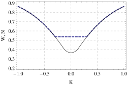
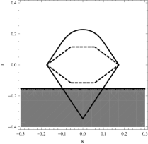
Figure 7: Left: Comparison of $W$ and $N$. Solid line is the plot of $W$ and dashed line is $N$. Right: Inside the dashed line region, LBP is guaranteed to converge by the Mooij’s condition. Inside the solid line, LBP is guaranteed to have the unique fixed point by Theorem 21. In the shaded region, LBP does not converges.

6 Analysis of stability of LBP

In this section, we analyze relations between the local stability of LBP and the local structure of the Bethe free energy around an LBP fixed point. Since LBP is not the gradient descent of the Bethe free energy function, such a relation is not necessarily obvious. From the view point of the variational formulation, we hope to find the minima. In the celebrated paper by Yedidia et al. (2001), they empirically found that locally stable LBP fixed points are local minima of the Bethe free energy function; Heskes (2002) have shown the fact for multinomial case.

In the following, we extend the result to two directions. First, we derive the conditions of the local stability and local minimality in terms of the eigenvalues of the matrix $\mathcal{M}(u)$, which immediately implies the above fact. Secondly, the result is extended to LBPs formulated by inference family including both multinomial and Gaussian cases. This is possible, since our analysis is based on the techniques developed in Section 4.

6.1 LBP as a dynamical system

First, we regard the LBP update as a dynamical system. At each time $t$, the state of the algorithm is specified by the set of messages $\{m_{\alpha\rightarrow i}^{t}\}$, which is identified with its natural parameters $\boldsymbol{\mu}^{t}=\{\mu_{\alpha\rightarrow i}^{t}\}\in\mathbb{R}^{\vec{E}}$. In terms of the parameters, the update rule Eq. (9) is written as follows.

$$\mu_{\alpha\rightarrow i}^{{t+1}}=\Lambda_{i}^{-1}\Big{(}\Lambda_{\alpha}(\bar{\theta}_{\alpha},\bar{\theta}^{\alpha}_{i_{1}}+\sum_{\beta\in N_{i_{1}}\smallsetminus\alpha}\mu^{t}_{\beta\rightarrow i_{1}},\ldots,\bar{\theta}^{\alpha}_{i_{k}}+\sum_{\beta\in N_{i_{k}}\smallsetminus\alpha}\mu^{t}_{\beta\rightarrow i_{k}})_{i}\Big{)}-\sum_{\gamma\in N_{i}\smallsetminus\alpha}\mu^{t}_{\gamma\rightarrow i},$$

where $\alpha=\{i_{1},\ldots,i_{d_{\alpha}}\}$, $d_{\alpha}=k$ and $\Lambda_{\alpha}(\cdots)_{i}$ is the $i$-th component ($i\in\alpha$). To obtain this equation, after multiply Eq. (9) by

$$\prod_{\gamma\in N_{i}\smallsetminus\alpha}m^{t}_{\gamma\rightarrow i}(x_{i}),$$

normalize it to be a probability density function, and then take the expectation of $\phi_{i}$.

Formally, this update rule can be viewed as a transform $T$ on the set of natural parameters of messages $M$:

$$T:M\longrightarrow M,\qquad\boldsymbol{\mu}^{t}=T(\boldsymbol{\mu}^{t-1}).$$

LBP algorithm can be formulated as repeated applications of this map. In this formulation, the fixed points of LBP are $\{\boldsymbol{\mu}^{*}\in M|\boldsymbol{\mu}^{*}=T(\boldsymbol{\mu}^{*})\}$.

Here we compute the differentiation of the update map $T$ around an LBP fixed point. This expression derived by Ikeda et al. (2004) for the cases of turbo and LDPC codes.

Theorem 23 (Differentiation of the LBP update)

At an LBP fixed point, the differentiation (linearization) of the LBP update is

$$\frac{\partial T(\boldsymbol{\mu})_{\alpha\rightarrow i}}{\partial\mu_{\beta\rightarrow j}}=\begin{cases}{\rm Var}_{b_{i}}[\phi_{i}]^{-1}{\rm Cov}_{b_{\alpha}}[\phi_{i},\phi_{j}]&\text{ if }j\in N_{\alpha}\smallsetminus i\text{ and }\beta\in N_{j}\smallsetminus\alpha,\\ 0&\text{ otherwise.}\end{cases}$$

In other words, at an LBP fixed point $\boldsymbol{\eta}\in L$, the differentiation of $T$ is

$$T^{\prime}=\mathcal{M}(\boldsymbol{u}),$$

where $\boldsymbol{u}=\{u^{\alpha}_{i\rightarrow j}\}$ is given by Eq. (24).

Proof  First, consider the case that $j\in N_{\alpha}\smallsetminus i\text{ and }\beta\in N_{j}\smallsetminus\alpha$. The derivative is equal to

$$\frac{\partial\Lambda^{-1}_{i}}{\partial\eta_{i}}\frac{\partial(\Lambda_{\alpha})_{i}}{\partial{\theta}_{\alpha:j}}={\rm Var}_{b_{i}}[\phi_{i}]^{-1}{\rm Cov}_{b_{\alpha}}[\phi_{i},\phi_{j}].$$

Another case is $i=j$ and $\alpha,\beta\in N_{i}~{}(\alpha\neq\beta)$. Then, the derivative is

$$\frac{\partial\Lambda^{-1}_{i}}{\partial\eta_{i}}\frac{\partial(\Lambda_{\alpha})_{i}}{\partial{\theta}_{\alpha:i}}-I=0$$

because ${\rm Var}_{b_{i}}[\phi_{i}]={\rm Var}_{b_{\alpha}}[\phi_{i}]$ from Eq. (13). In other cases, the derivative is trivially zero.  

The relation $j\in N_{\alpha}\smallsetminus i\text{ and }\beta\in N_{j}\smallsetminus\alpha$ will be written as $(\beta\rightarrow j)\rightharpoonup(\alpha\rightarrow i)$ in Subsection 3.1. It is noteworthy that the elements of the linearization matrix is explicitly expressed by the fixed point beliefs.

6.2 Spectral conditions

Let $T$ be the LBP update map. A fixed point $\boldsymbol{\mu}^{*}$ is called locally stable if LBP starting with a point sufficiently close to $\boldsymbol{\mu}^{*}$ converges to $\boldsymbol{\mu}^{*}$. To suppress oscillatory behaviors of LBP, damping of update $T_{\epsilon}:=(1-\epsilon)T+\epsilon I$ is sometimes useful, where $0\leq\epsilon<1$ is a damping strength and $I$ is the identity matrix.

As we will summarize in the following theorem, the local stability is determined by the linearization $T^{\prime}$ at the fixed point. Since $T^{\prime}$ is nothing but $\mathcal{M}(\boldsymbol{u})$ at an LBP fixed point, Theorem 14 implies relations between the local stability and the Hessian of the Bethe free energy function.

Theorem 24

Let $\boldsymbol{\mu}^{*}$ be an LBP fixed point and assume that $T^{\prime}(\boldsymbol{\mu}^{*})$ has no eigenvalues of unit modulus for simplicity. Then the following statements hold.

1. ${\rm Spec}(T^{\prime}(\boldsymbol{\mu}^{*}))\subset\{\lambda\in\mathbb{C}||\lambda|<1\}$ $\iff$ LBP is locally stable at $\boldsymbol{\mu}^{*}$.

2. ${\rm Spec}(T^{\prime}(\boldsymbol{\mu}^{*}))\subset\{\lambda\in\mathbb{C}|{\rm Re}\lambda<1\}$ $\iff$ LBP is locally stable at $\boldsymbol{\mu}^{*}$ with some damping.

3. ${\rm Spec}(T^{\prime}(\boldsymbol{\mu}^{*}))\subset\mathbb{C}\smallsetminus\mathbb{R}_{\geq 1}$ $\Rightarrow$ $\boldsymbol{\mu}^{*}$ is a local minimum of the Bethe free energy function.

Proof  $1.:$ This is a standard result. (See Guckenheimer and Holmes (1990) for example.)  $2.:$ There is an $\epsilon\in[0,1)$ that satisfy ${\rm Spec}(T_{\epsilon}^{\prime}(\boldsymbol{\mu}^{*}))\subset\{\lambda\in\mathbb{C}||\lambda|<1\}$ if and only if ${\rm Spec}(T^{\prime}(\boldsymbol{\mu}^{*}))\subset\{\lambda\in\mathbb{C}|{\rm Re}\lambda<1\}$.  $3.:$ This assertion is a direct consequence of Theorem 14 and 23.  

This theorem immediately implies that a locally stable LBP fixed point is a local minimum of the Bethe free energy. The theorem applies to both the multinomial and Gaussian cases.

It is interesting to ask under which condition a local minimum of the Bethe free energy function is a locally stable fixed point of (damped) LBP. An implicit reason for the empirical success of the LBP algorithm is that LBP finds a “good” local minimum rather than a local minimum nearby the initial point. The theorem gives a new insight to the question, i.e., the difference between the stable local minima and the unstable local minima in terms of the spectrum of $T^{\prime}(\boldsymbol{\mu}^{*})$.

6.3 Special cases: gaps between stability and local minimality

Here we focus on two special cases: binary pairwise attractive models and pairwise fixed-mean Gaussian models. Note that a binary pairwise graphical model $\Psi=\{\Psi_{ij},\Psi_{i}\}$ is called attractive if $J_{ij}\geq 0$, where $\Psi_{i}(x_{i})=\exp(h_{i}x_{i})$ and $\Psi_{ij}(x_{i},x_{j})=\exp(J_{ij}x_{i}x_{j})$ $~{}(x_{i},x_{j}\in\{\pm 1\})$. In these cases, the stable fixed points of LBP and the local minima of Bethe free energy function are less different.

Consider the following situation: we have continuously parametrized compatibility functions $\{\Psi_{ij}(t),\Psi_{i}(t)\}_{t\geq 0}$, which are constants at $t=0$ (e.g. $t$ is a inverse temperature: $\Psi_{ij}(t)=\exp(tJ_{ij}x_{i}x_{j})$ and $\Psi_{i}(t)=\exp(th_{i}x_{i})$). Starting from $t=0$, we run LBP algorithm for $t$, find a stable fixed point and use it as initial messages of LBP for $t+\delta t$, where $\delta t$ is a sufficiently small positive number. Then we obtain a trajectory of a stable fixed point beliefs: we call it a belief trajectory. It first continuously follow the local minima and then it may jump to another stable fixed point belief at $t=t_{0}$. The following theorem implies that the stable fixed point becomes unstable by continuous changes of the compatibility functions exactly when the corresponding local minimum becomes a saddle.

Theorem 25

Suppose that we have a continuously parametrized compatibility functions of attractive binary pairwise model or fixed-mean Gaussian model as above. If the LBP fixed point becomes unstable across $t=t_{0}$ for the first time following the belief trajectory, then the corresponding local minimum of the Bethe free energy becomes a saddle point across $t=t_{0}$.

Proof  First consider the case of attractive binary pairwise models. From Eq. (11), we see that $b_{ij}(x_{i},x_{j})\propto\exp(J_{ij}x_{i}x_{j}+\theta_{i}x_{i}+\theta_{j}x_{j})$ for some $\theta_{i}$ and $\theta_{j}$. From $J_{ij}\geq 0$, we have ${\rm Cov}_{b_{ij}}[x_{i},x_{j}]\geq 0$, and thus $u_{i\rightarrow j}\geq 0$. When the LBP fixed point becomes unstable, the Perron-Frobenius eigenvalue of $\mathcal{M}(\boldsymbol{u})$ goes over $1$, which means $\det(I-\mathcal{M}(\boldsymbol{u}))$ crosses $0$. From Theorem 11, we see that $\det(\nabla^{2}F)$ becomes positive to negative at $t=t_{0}$. The Gaussian case can be proved analogously. Recall that the weight $u_{i\rightarrow j}$ are always positive scalars as shown in Corollary 13.  

Theorem 25 extends Theorem 2 of Mooij and Kappen (2005), which discusses only the case of binary pairwise models with vanishing local fields $h_{i}=0$ and the trivial fixed point (i.e. ${\rm E}_{b_{i}}[x_{i}]=0$).

7 Summary and discussions

We have established a connection between graph zeta function, Bethe free energy and loopy belief propagation. We have shown that this connection provides powerful tools for the analysis of Bethe free energy and LBP; key theorems are given in Section 4. In Section 5, based on the theorems, we analyzed the (non) convexity of the Bethe free energy function. Roughly speaking, the positive definite region of Bethe free energy functions shrinks as the Perron-Frobenius eigenvalue of the directed edge matrix becomes large, or equivalently, as the pole of the Ihara zeta function closest to the origin approaches to zero. We have shown that such knowledge can be used to derive the uniqueness property of LBP. In Section 6, we have shown that the local stability of LBP implies local minimality of Bethe free energy as long as LBP is well defined within a class of exponential families. A key observation is that the matrix $\mathcal{M}(\boldsymbol{u})$ is equal to the linearization of the LBP update at LBP fixed points.

The Bethe-zeta formula shows that the Bethe free energy function contains information on the graph geometry, especially on the prime cycles. The formula helps extract graph information from the Bethe free energy function. For example we observed that the number of the spanning trees are derived from a limit of the Bethe free energy function. In a sense, the connection between those three objects seems to be natural as all of them becomes “trivial” if the associated graph structure is a tree. If the associated hypergraph is a tree, zeta function is equal to $1$, Bethe free energy function is equal to the Gibbs free energy function and LBP reduces to the original BP, which computes exact marginals in finite steps.

7.1 Path forward

In this subsection, we list a few directions of future researches going beyond the results of this paper.

In a sequel paper (Watanabe and Fukumizu, 2011), we further exploit the connection between LBP, Bethe free energy and graph zeta function to analyze the LBP fixed point equation, focusing on binary pairwise models. We characterize the class of signed graph on which uniqueness of the LBP fixed point is guaranteed. Note that the signs on the edges represents those of the interactions (i.e. $\operatorname*{sgn}J_{ij}$). The condition is contrast to the those of the past researches and the result in Section 5, where the strength of interactions (i.e. $|J_{ij}|$) are bounded.

In Subsection 5.2, we have derived a condition for the convexity for the restricted Bethe free energy function. Unfortunately, the expression of the weight $W$ involves $\sup$ operator and does not easy to compute directly. We need further consideration to find a way of compute it more easily. The proof of the conjecture $W\leq N$ is also an interesting problem.

The connection between graph zeta, Bethe free energy and LBP can be extended to a more general class of free energies including fractional and tree-reweighted types (Wiegerinck and Heskes, 2003; Wainwright et al., 2003b). These free energies are obtained by modifying the coefficients in the definition of the Bethe free energy function. The corresponding graph zeta function then becomes the Bartholdi type, which allows cycles with backtracking (Bartholdi, 1999; Iwao, 2006). The relation may be useful to analyze such class of free energies.

Acknowledgments

This work was supported in part by Grant-in-Aid for JSPS Fellows 20-993 and Grant-in-Aid for Scientific Research (C) 22300098.

A

A.1 Miscellaneous properties of one-variable hypergraph zeta function

This subsection provides miscellaneous facts related to the one-variable hypergraph zeta functions. In the analyses of this paper, we sometimes reduce the multivariate zeta to the one-variable zeta. Therefore, it is important to understand the one-variable hypergraph zeta $\zeta_{H}(u)$ and the directed edge matrix $\mathcal{M}$.

Recall that $\rho(X)$ denotes the spectral radius of $X$. We have the following bounds on the spectral radius of $\mathcal{M}$.

Proposition 26

For $e\in\vec{E}$, let $k_{e}:=|\{e^{\prime}\in\vec{E};e^{\prime}\rightharpoonup e\}|$, $k_{m}=\min k_{e}$ and $k_{M}=\max k_{e}$. Then

$$k_{m}\leq\rho(\mathcal{M})\leq k_{M}.$$

Therefore, if $H$ is a graph,

$$\min_{i\in V}d_{i}-1\leq\rho({\mathcal{M}})\leq\max_{i\in V}d_{i}-1.$$ (30)

Proof Since $k_{e}=\sum_{e^{\prime}}\mathcal{M}_{e,e^{\prime}}$, the bound is trivial from the easy bound on the spectral radius of non-negative matrices. See Theorem 8.1.22 of Horn and Johnson (1990).  
Since the directed matrix $\mathcal{M}$ is non-negative, the spectral radius is equal to the Perron-Frobenius eigenvalue. The pole of $\zeta_{H}$ closest to the origin is $u=\rho(\mathcal{M})^{-1}\geq k_{M}^{-1}$. For the case of Ihara’s zeta function, a bound on the modulus of imaginary poles as well as Eq. (30) are given by Kotani and Sunada (2000).

For arbitrary hypergraph, $\zeta_{H}(u)$ has a pole at $u=1$ because $\det(I-\mathcal{M})=0$. The following theorem gives the multiplicity of the pole. The original version of this theorem is proved by Hashimoto (1989, 1990).

Theorem 27 (Hypergraph Hashimoto’s theorem (Hashimoto, 1989; Storm, 2006))

Let $\chi(H):=|V|+|F|-|\vec{E}|$ be the Euler number of $H$.

$$\lim_{u\rightarrow 0}\zeta_{H}(u)^{-1}(1-u)^{-\chi(H)+1}=\chi(H)\kappa(B_{H}),$$

where $\kappa(B_{H})$ is the number of spanning trees of the bipartite graph $B_{H}$. ($B_{H}$ is the bipartite graph representation of the hypergraph $H$.)

Proof For a graph $G=(V,E)$, Hashimoto (1989, 1990) proved that

$$\lim_{u\rightarrow 1}Z_{G}(u)^{-1}(1-u)^{-|E|+|V|-1}=-2^{|E|-|V|+1}(|E|-|V|)\kappa(G),$$

where $\kappa(G)$ is the number of spanning tree of $G$. A simple proof is given by Northshield (1998). Since there is a one-to-one correspondence between $\mathfrak{P}_{H}$ and $\mathfrak{P}_{B_{H}}$, we have $\zeta_{H}(u)=Z_{B_{H}}(\sqrt{u})$. Then the assertion is proved from the above formula.  

A.2 Detailed Proofs

Proof of Theorem 4  The conditions for stationary points of the Bethe free energy function are ${{\bar{\theta}}_{\langle\alpha\rangle}}={{\theta}_{\langle\alpha\rangle}}$ and $\sum_{\alpha\ni i}(-{\bar{\theta}}_{\alpha:i}+{\theta}_{\alpha:i})+(1-d_{i})\theta_{i}=0$.
$(1.\Rightarrow 2.)$ The correspondence from the fixed point message to the stationary point is given by Eqs. (10,11). From this construction, we see that

$$\prod_{\alpha\in F}\Psi_{\alpha}(x_{\alpha})\propto\prod_{\alpha}b_{\alpha}(x_{\alpha})\prod_{i}b_{i}(x_{i})^{1-d_{i}}.$$

This implies the above stationary point conditions.
$(2.\Rightarrow 1.)$ The converse correspondence is given by $m_{\alpha\rightarrow i}(x_{i})=\exp(\langle\theta_{i}+{\bar{\theta}}_{\alpha:i}-{\theta}_{\alpha:i},\phi_{i}\rangle)$, where $\{{{\theta}_{\alpha}},\theta_{i}\}$ are the natural parameters of the stationary point pseudomarginals $\{b_{\alpha}(x_{\alpha}),b_{i}(x_{i})\}$. From this construction and the stationary point conditions, we have

$$\prod_{\beta\in N_{i}}m_{\beta\rightarrow i}(x_{i})=\exp(\langle\theta_{i},\phi_{i}(x_{i})\rangle)\propto b_{i}(x_{i}),$$

$$\Psi_{\alpha}(x_{\alpha})\prod_{i\in\alpha}\prod_{\beta\in N_{i}\smallsetminus\alpha}m_{\beta\rightarrow i}(x_{i})=\exp(\langle{{\theta}_{\langle\alpha\rangle}},{{\phi}_{\langle\alpha\rangle}}(x_{\alpha})\rangle+\sum_{i\in N_{\alpha}}\langle{\theta}_{\alpha:i},\phi_{i}\rangle)\propto b_{\alpha}(x_{\alpha}).$$

Therefore, the local consistency condition Eq. (13) implies that

$$\prod_{\beta\in N_{i}}m_{\beta\rightarrow i}(x_{i})\propto\int\Psi_{\alpha}\prod_{j\in\alpha}\prod_{\beta\in N_{j}\smallsetminus\alpha}m_{\beta\rightarrow j}(x_{j}){\rm d}\nu_{\alpha\smallsetminus i}.$$

This is equivalent to the LBP fixed point equation.

$\square$

Proof of Theorem 6  The following proof proceeds in an analogous manner with Theorem 3 in Stark and Terras (1996). First define a differential operator

$$\mathcal{H}:=\sum_{e^{\prime}\rightharpoonup e}\sum_{a_{e},a_{e^{\prime}}}(u_{e^{\prime}\rightharpoonup e})_{a_{e},a_{e^{\prime}}}\frac{\partial}{\partial(u_{e^{\prime}\rightharpoonup e})_{a_{e},a_{e^{\prime}}}}$$

where $(u_{e^{\prime}\rightharpoonup e})_{a_{e},a_{e^{\prime}}}$ denotes the $(a_{e},a_{e^{\prime}})$ element of the matrix $u_{e^{\prime}\rightharpoonup e}$. If we apply this operator to a $k$ product of $u$ terms, it is multiplied by $k$. Since $\log\zeta_{H}(\boldsymbol{0})=0$ and $\log\det(I-\mathcal{M}(\boldsymbol{0}))^{-1}=0$, it is enough to prove that $\mathcal{H}\log\zeta_{H}(\boldsymbol{u})=\mathcal{H}\log\det(I-\mathcal{M}(\boldsymbol{u}))^{-1}$. Using equations $\log\det X={\rm tr}\log X$ and $-\log(1-x)=\sum_{k\geq 1}\frac{1}{k}x^{k}$, we have

$$\mathcal{H}\log\zeta_{H}(\boldsymbol{u}) =\mathcal{H}\sum_{\mathfrak{p}\in\mathfrak{P}_{H}}-\log\det(I-\pi(\mathfrak{p}))$$

$$=\mathcal{H}\sum_{\mathfrak{p}\in\mathfrak{P}_{H}}\sum_{k\geq 1}\frac{1}{k}{\rm tr}(\pi(\mathfrak{p})^{k})$$ (31)

$$=\sum_{\mathfrak{p}\in\mathfrak{P}_{H}}\sum_{k\geq 1}|\mathfrak{p}|{\rm tr}(\pi(\mathfrak{p})^{k})$$ (32)

$$=\sum_{C:\text{closed geodesic}}{\rm tr}(\pi(C))\quad=\sum_{k\geq 1}{\rm tr}(\mathcal{M}(\boldsymbol{u})^{k}).$$

From Eq. (31) to Eq. (32), notice that $\mathcal{H}$ acts as a multiplication of $k|\mathfrak{p}|$ for each summand. This is because the summand is a sum of degree $k|\mathfrak{p}|$ terms counting each $(u_{e^{\prime}\rightharpoonup e})_{a_{e},a_{e^{\prime}}}$ degree one.

On the other hand, one easily observes that

$$\mathcal{H}\log\det(I-\mathcal{M}(\boldsymbol{u}))^{-1} =\mathcal{H}\sum_{k\geq 1}\frac{1}{k}{\rm tr}(\mathcal{M}(\boldsymbol{u})^{k})$$

$$=\sum_{k\geq 1}{\rm tr}(\mathcal{M}(\boldsymbol{u})^{k}).$$

Thus, the proof is completed.

$\square$

Proof of Theorem 7

The proof is based on the decomposition in the following lemma and determinant manipulations. We define a linear operator by

$$\mathcal{T}:\mathfrak{X}(V)\rightarrow\mathfrak{X}(\vec{E}),\qquad (\mathcal{T}g)(e):=g(t(e))$$

The vector spaces $\mathfrak{X}(\vec{E})$ and $\mathfrak{X}(V)$ have inner products naturally. We can think of the adjoint of $\mathcal{T}$ which is given by

$$\mathcal{T}^{*}:\mathfrak{X}(\vec{E})\rightarrow\mathfrak{X}(V),\qquad(\mathcal{T}^{*}f)(i):=\sum_{e:t(e)=i}f(e).$$

These linear operators have the following relation.

Lemma

$$\mathcal{M}(\boldsymbol{u})=\boldsymbol{\iota}(\boldsymbol{u})\mathcal{T}\mathcal{T}^{*}-\boldsymbol{\iota}(\boldsymbol{u})$$

Proof [Proof of Lemma] Let $f\in\mathfrak{X}(V)$.

$$\Big{(}\boldsymbol{\iota}(\boldsymbol{u})\mathcal{T}\mathcal{T}^{*}-\boldsymbol{\iota}(\boldsymbol{u})\Big{)}f(e) =\sum_{e^{\prime}:{s(e^{\prime})=s(e)\atop t(e^{\prime})\neq t(e)}}u^{s(e)}_{t(e^{\prime})\rightarrow t(e)}\sum_{e^{\prime\prime}:t(e^{\prime\prime})=t(e^{\prime})}f(e^{\prime\prime})-\sum_{e^{\prime\prime}:{s(e^{\prime\prime})=s(e)\atop t(e^{\prime\prime})\neq t(e)}}u^{s(e)}_{t(e^{\prime\prime})\rightarrow t(e)}f(e^{\prime\prime})$$

$$=\sum_{e^{\prime}:{s(e^{\prime})=s(e)\atop t(e^{\prime})\neq t(e)}}u^{s(e)}_{t(e^{\prime})\rightarrow t(e)}\sum_{e^{\prime\prime}:{t(e^{\prime\prime})=t(e^{\prime})\atop e^{\prime\prime}\neq e^{\prime}}}f(e^{\prime\prime})$$

$$=(\mathcal{M}(\boldsymbol{u})f)(e).$$

 

Using this lemma, we have

$$\zeta_{G}(\boldsymbol{u})^{-1} =\det(I-\mathcal{M}(\boldsymbol{u}))$$

$$=\det(I-\boldsymbol{\iota}(\boldsymbol{u})\mathcal{T}\mathcal{T}^{*}+\boldsymbol{\iota}(\boldsymbol{u}))$$

$$=\det(I-\boldsymbol{\iota}(\boldsymbol{u})\mathcal{T}\mathcal{T}^{*}(I+\boldsymbol{\iota}(\boldsymbol{u}))^{-1})\det((I+\boldsymbol{\iota}(\boldsymbol{u})))$$

$$=\det(I_{r_{V}}-\mathcal{T}^{*}(I+\boldsymbol{\iota}(\boldsymbol{u}))^{-1}\boldsymbol{\iota}(\boldsymbol{u})\mathcal{T})\prod_{\alpha\in F}\det(U_{\alpha})$$

It is easy to see that $I_{r_{V}}-\mathcal{T}^{*}(I+\boldsymbol{\iota}(\boldsymbol{u}))^{-1}\boldsymbol{\iota}(\boldsymbol{u})\mathcal{T}=I_{r_{V}}-\mathcal{T}^{*}\mathcal{T}+\mathcal{T}^{*}(I+\boldsymbol{\iota}(\boldsymbol{u}))^{-1}\mathcal{T}$. We also see that

$$(\mathcal{T}^{*}\mathcal{T}g)(i)=\sum_{e:t(e)=i}g(t(e))=d_{i}g(i)$$

and

$$(\mathcal{T}^{*}(I+\boldsymbol{\iota}(\boldsymbol{u}))^{-1}\mathcal{T}g)(i)=\sum_{e:t(e)=i}((I+\boldsymbol{\iota}(\boldsymbol{u}))^{-1}\mathcal{T}g)(e)=(\mathcal{W}g)(i).$$

$\square$

Proof of Proposition 16  The right inequality is obvious. We prove the left inequality. Let $C=\rho(\mathcal{M}(\|\boldsymbol{u}\|))$. It is enough to prove that $\det(I-z\mathcal{M}(\boldsymbol{u}))$ has no root in $\{\lambda\in\mathbb{C}|\hskip 5.69054pt|\lambda|<C^{-1}\}$. Accordingly, we show that $\zeta_{H}(z\boldsymbol{u})$ has no pole in the set. Let $\mathfrak{p}$ be a prime cycle and let $\lambda_{1},\ldots,\lambda_{r}$ be the eigenvalues of $\pi(\mathfrak{p};\boldsymbol{u})$. Then we obtain $\max|\lambda_{l}|\leq\pi(\mathfrak{p};\|\boldsymbol{u}\|)$. Therefore, if $|z|<\pi(\mathfrak{p};\|\boldsymbol{u}\|)^{-1}$, we have

$$\left|\det(I-z^{|\mathfrak{p}|}\pi(\mathfrak{p};\boldsymbol{u}))\right|=\left|\prod_{l}(1-z^{|\mathfrak{p}|}\lambda_{l})\right|\geq\Big{(}1-|z|^{|\mathfrak{p}|}\pi(\mathfrak{p};\|\boldsymbol{u}\|)\Big{)}^{r}.$$

It is not difficult to see that, for arbitrary prime cycle $\mathfrak{p}$, an inequality $C^{-1}\leq\pi(\mathfrak{p};\|\boldsymbol{u}\|)^{-1}$ holds. Therefore, if $|z|<C^{-1}$,

$$\left|\zeta_{H}(z\boldsymbol{u})\right|=\left|\prod_{\mathfrak{p}\in P}\det(I-z^{|\mathfrak{p}|}\pi(\mathfrak{p};\boldsymbol{u}))^{-1}\right|\leq\prod_{\mathfrak{p}\in P}\Big{(}1-|z|^{|\mathfrak{p}|}\pi(\mathfrak{p};\|\boldsymbol{u}\|)\Big{)}^{-r}=\zeta_{H}(|z|\|\boldsymbol{u}\|)^{r}<\infty.$$

$\square$

Proof of Theorem 18 (ii) : Multinomial case  First, we consider binary case, i.e. $\phi_{i}(x_{i})=x_{i}\in\{\pm 1\}$. For $t\in[0,1]$, let us define $\eta_{ij}(t)={\rm E}_{b_{\alpha}}[x_{i}x_{j}]=t$ and $\eta_{i}(t)=0$. Accordingly, $u^{\alpha}_{i\rightarrow j}=t$ and $\boldsymbol{\eta}(t)\in L$. As $t\nearrow 1$, $\boldsymbol{\eta}(t)$ approaches to a boundary point of $L$. Using Theorem 27, analogous to the fixed-mean Gaussian case, we see that $\det(\nabla^{2}F(t))$ becomes negative as $t\rightarrow 1$ if $n(H)>1$. Therefore, $F$ is not convex on $L$.

For general multinomial inference families, the non convexity of $F$ is deduced from the binary case. There is a face of (the closure of) $L$ that is identified with the set of pseudomarginals of the binary inference family on the same hypergraph. Since $0\log 0=0$, we see that the restriction of $F$ on the face is the Bethe free energy function of the binary inference family. Since this restriction is not convex, $F$ is not convex.

$\square$

References

- An (1988) G. An. A note on the cluster variation method. Journal of Statistical Physics, 52(3):727–734, 1988.
- Baron et al. (2010) D. Baron, S. Sarvotham, and R.G. Baraniuk. Bayesian compressive sensing via belief propagation. Signal Processing, IEEE Transactions on, 58(1):269–280, 2010.
- Bartholdi (1999) L. Bartholdi. Counting paths in graphs. Enseign. Math., II. Sér., 45(1-2):83–131, 1999.
- Bass (1992) H. Bass. The Ihara-Selberg zeta function of a tree lattice. Internat. J. Math, 3(6):717–797, 1992.
- Bethe (1935) H.A. Bethe. Statistical theory of superlattices. Proc. R. Soc. Lon. A, 150(871):552–575, 1935.
- Foata and Zeilberger (1999) D. Foata and D. Zeilberger. A combinatorial proof of Bass’s evaluations of the Ihara-Selberg zeta function for graphs. Transactions of the American Mathematical Society, 351(6):2257–2274, 1999.
- Guckenheimer and Holmes (1990) J. Guckenheimer and P. Holmes. Nonlinear oscillations, dynamical systems, and bifurcations of vector fields. Springer, 1990.
- Hashimoto (1989) K. Hashimoto. Zeta functions of finite graphs and representations of p-adic groups. Automorphic forms and geometry of arithmetic varieties, 15:211–280, 1989.
- Hashimoto (1990) K. Hashimoto. On zeta and L-functions of finite graphs. Internat. J. Math, 1(4):381–396, 1990.
- Heskes (2002) T. Heskes. Stable fixed points of loopy belief propagation are minima of the Bethe free energy. Advances in Neural Information Processing Systems, 15, pages 343–350, 2002.
- Heskes (2004) T. Heskes. On the uniqueness of loopy belief propagation fixed points. Neural Computation, 16(11):2379–2413, 2004.
- Horn and Johnson (1990) R.A. Horn and C.R. Johnson. Matrix analysis. Cambridge University Press, 1990.
- Horton et al. (2008) M.D. Horton, H.M. Stark, and A.A. Terras. Zeta Functions of weighted graphs and covering graphs. Analysis on Graphs and Its Applications, 77:29, 2008.
- Ihara (1966) Y. Ihara. On discrete subgroups of the two by two projective linear group over p-adic fields. Journal of the Mathematical Society of Japan, 18(3):219–235, 1966.
- Ihler et al. (2005) A.T. Ihler, J.W. Fisher III, R.L. Moses, and A.S. Willsky. Nonparametric belief propagation for self-localization of sensor networks. Selected Areas in Communications, IEEE Journal on, 23(4):809–819, 2005. ISSN 0733-8716.
- Ihler et al. (2006) A.T. Ihler, J.W. Fisher III, and A.S. Willsky. Loopy belief propagation: Convergence and effects of message errors. Journal of Machine Learning Research, 6(1):905–936, 2006.
- Ikeda et al. (2004) S. Ikeda, T. Tanaka, and S. Amari. Information geometry of turbo and low-density parity-check codes. IEEE Transactions on Information Theory, 50(6):1097–1114, 2004.
- Iwao (2006) S. Iwao. Bartholdi zeta functions for hypergraphs. The Electronic Journal of Combinatorics, 14(1):N2, 2006.
- Johnson et al. (2006) J. Johnson, D. Malioutov, and A. Willsky. Walk-sum interpretation and analysis of Gaussian belief propagation. Advances in Neural Information Processing Systems, 18:579, 2006.
- Jordan (1998) M.I. Jordan. Learning in graphical models. Kluwer Academic Publishers, 1998.
- Kotani and Sunada (2000) M. Kotani and T. Sunada. Zeta functions of finite graphs. Journal of Mathematical Sciences. The University of Tokyo, 7(1):7–25, 2000.
- Kschischang et al. (2001) F.R. Kschischang, B.J. Frey, and H.A. Loeliger. Factor graphs and the sum-product algorithm. IEEE Transactions on information theory, 47(2):498–519, 2001.
- Malioutov et al. (2006) D.M. Malioutov, J.K. Johnson, and A.S. Willsky. Walk-sums and belief propagation in Gaussian graphical models. The Journal of Machine Learning Research, 7:2064, 2006.
- Mardia et al. (2009) K.V. Mardia, J.T. Kent, G. Hughes, and C.C. Taylor. Maximum likelihood estimation using composite likelihoods for closed exponential families. Biometrika, 96(4):975–982, 2009.
- McEliece et al. (1998) R.J. McEliece, D.J.C. MacKay, and J.F. Cheng. Turbo decoding as an instance of Pearl’s ”belief propagation” algorithm. IEEE J. Sel. Areas Commun., 16(2):140–52, 1998.
- Mezard et al. (2002) M. Mezard, G. Parisi, and R. Zecchina. Analytic and algorithmic solution of random satisfiability problems. Science, 297(5582):812, 2002.
- Mizuno and Sato (2004) H. Mizuno and I. Sato. Weighted zeta functions of graphs. Journal of Combinatorial Theory, Series B, 91(2):169–183, 2004.
- Mooij and Kappen (2005) J.M. Mooij and H.J. Kappen. On the properties of the Bethe approximation and loopy belief propagation on binary networks. Journal of Statistical Mechanics: Theory and Experiment, 11:P11012, 2005.
- Mooij and Kappen (2007) J.M. Mooij and H.J. Kappen. Sufficient conditions for convergence of the sum-product algorithm. IEEE Transactions on Information Theory, 53(12):4422–4437, 2007.
- Murphy et al. (1999) K. Murphy, Y. Weiss, and M.I. Jordan. Loopy belief propagation for approximate inference: An empirical study. Proc. of Uncertainty in AI, 15:467–475, 1999.
- Northshield (1998) S. Northshield. A note on the zeta function of a graph. Journal of Combinatorial Theory, Series B, 74(2):408–410, 1998.
- Pakzad and Anantharam (2002) P. Pakzad and V. Anantharam. Belief propagation and statistical physics. Conference on Information Sciences and Systems, 2002.
- Pearl (1988) J. Pearl. Probabilistic Reasoning in Intelligent Systems: Networks of Plausible Inference. Morgan Kaufmann Publishers, San Mateo, CA, 1988.
- Pelizzola (2005) A. Pelizzola. Cluster variation method in statistical physics and probabilistic graphical models. Journal of Physics A: Mathematical General, 38(33):R309–R339, 2005.
- Serre (1980) J.P. Serre. Trees. Springer-Verlag, 1980.
- Stark and Terras (1996) H.M. Stark and A.A. Terras. Zeta functions of finite graphs and coverings. Advances in Mathematics, 121(1):124–165, 1996.
- Storm (2006) C.K. Storm. The zeta function of a hypergraph. The Electronic Journal of Combinatorics, 13(R84):1, 2006.
- Sudderth et al. (2002) E.B. Sudderth, A.T. Ihler, W.T. Freeman, and A.S. Willsky. Nonparametric belief propagation and facial appearance estimation. In IEEE International Conference on Computer Vision and Pattern Recognition, pages 605–612, 2002.
- Sunada (1986) T. Sunada. L-functions in geometry and some applications. Lecture Notes in Math, 1201:266–284, 1986.
- Tatikonda and Jordan (2002) S. Tatikonda and M.I. Jordan. Loopy belief propagation and Gibbs measures. Uncertainty in AI, 18:493–500, 2002.
- Venkataraman (2009) P. Venkataraman. Applied optimization with MATLAB programming. John Wiley and Sons, 2009.
- Wainwright et al. (2003a) M.J. Wainwright, T.S. Jaakkola, and A.S. Willsky. Tree-based reparameterization framework for analysis of sum-product and related algorithms. IEEE Transactions on Information Theory, 49(5):1120–1146, 2003a.
- Wainwright et al. (2003b) M.J. Wainwright, T.S. Jaakkola, and A.S. Willsky. Tree-reweighted belief propagation algorithms and approximate ML estimation by pseudomoment matching. In Workshop on Artificial Intelligence and Statistics, volume 21, 2003b.
- Wainwright et al. (2005) M.J. Wainwright, T.S. Jaakkola, and A.S. Willsky. MAP estimation via agreement on trees: message-passing and linear programming. IEEE Transactions on Information Theory, 51(11):3697–3717, 2005.
- Wainwright and Jordan (2003) M.J. Wainwright and M.I. Jordan. Variational inference in graphical models: The view from the marginal polytope. In proceedings of the annual Allerton Conference on Communication, Control, and Computing, volume 41, pages 961–971, 2003.
- Wainwright and Jordan (2008) M.J. Wainwright and M.I. Jordan. Graphical models, exponential families, and variational inference. Foundations and Trends in Machine Learning, 1(1-2):1–305, 2008.
- Watanabe and Fukumizu (2011) W. Watanabe and K. Fukumizu. On the uniquness of the solution of belief propagation equation. in preparation, 2011.
- Watanabe (2010) Y Watanabe. Discrete geometric analysis of message passing algorithm on graphs. Ph.D thesis, 2010.
- Watanabe and Fukumizu (2009) Y. Watanabe and K. Fukumizu. Graph zeta function in the Bethe free energy and loopy belief propagation. Advances in Neural Information Processing Systems, 2009.
- Weiss (2000) Y. Weiss. Correctness of local probability propagation in graphical models with loops. Neural Computation, 12(1):1–41, 2000.
- Weiss et al. (2007) Y. Weiss, C. Yanover, and T. Meltzer. MAP estimation, linear programming and belief propagation with convex free energies. Uncertainty in Artificial Intelligence, 2007.
- Whittaker (2009) J. Whittaker. Graphical models in applied multivariate statistics. Wiley Publishing, 2009.
- Wiegerinck and Heskes (2003) W. Wiegerinck and T. Heskes. Fractional belief propagation. Advances in Neural Information Processing Systems, pages 455–462, 2003.
- Yedidia et al. (2001) J.S. Yedidia, W.T. Freeman, and Y. Weiss. Generalized belief propagation. Advances in Neural Information Processing Systems, 13:689–95, 2001.
- Yedidia et al. (2005) J.S. Yedidia, W.T. Freeman, and Y. Weiss. Constructing free-energy approximations and generalized belief propagation algorithms. IEEE Transactions on Information Theory, 51(7):2282–2312, 2005.