Bayesian Model Choice of Grouped t-copula

Abstract

One of the most popular copulas for modeling dependence structures is $t$-copula. Recently the grouped $t$-copula was generalized to allow each group to have one member only, so that a priori grouping is not required and the dependence modeling is more flexible. This paper describes a Markov chain Monte Carlo (MCMC) method under the Bayesian inference framework for estimating and choosing $t$-copula models. Using historical data of foreign exchange (FX) rates as a case study, we found that Bayesian model choice criteria overwhelmingly favor the generalized $t$-copula. In addition, all the criteria also agree on the second most likely model and these inferences are all consistent with classical likelihood ratio tests. Finally, we demonstrate the impact of model choice on the conditional Value-at-Risk for portfolios of six major FX rates.

Key words: grouped $t-$copula, dependence modeling, Bayesian model choice, Markov chain Monte Carlo, foreign exchange.

¹ CSIRO Mathematics, Informatics and Statistics, Australia; e-mail: Xiaolin.Luo@csiro.au
² CSIRO Mathematics, Informatics and Statistics, Australia; e-mail: Pavel.Shevchenko@csiro.au
^∗ Corresponding author

1 Introduction

Copula functions have become popular and flexible tools in modeling multivariate dependence among financial risk factors. In practice, one of the most popular copulas in modeling multivariate financial data is perhaps the $t$-copula implied by the multivariate $t$-distribution (hereafter referred to as standard t-copula); see Embrechts et al (2001), Fang et al (2002), and Demarta and McNeil (2005). This is due to its simplicity in terms of simulation and calibration, combined with its ability to model tail dependence which is often observed in financial returns data. Papers by Mashal et al (2003) and Breymann et al (2003) have demonstrated that the empirical fit of the standard $t$-copula is superior in most cases when compared to the Gaussian copula. However, the standard $t$-copula is often criticized due to the restriction of having only one parameter for the degrees of freedom (dof), which may limit its ability to model tail dependence in multivariate case. To overcome this problem, Daul et al (2003) proposed the use of the grouped t-copula, where risks are grouped into classes and each class has its own standard $t$-copula with a specific dof. This, however, requires an a priori choice of classes. It is not always obvious how the risk factors should be divided into sub-groups. An adequate choice of grouping configurations requires substantial additional effort if there is no natural grouping, for example, by sector or class of asset.

Recently, the grouped $t$-copula was generalized to a new $t$-copula with multiple dof parameters (hereafter referred to as generalized t-copula); see Luo and Shevchenko (2010) and Venter et al (2007). This copula can be viewed as a grouped $t$-copula with each group having only one member. It has the advantages of a grouped $t$-copula with flexible modeling of multivariate dependences, yet at the same time it overcomes the difficulties with a priori choice of groups. For convenience, denote the new copula as $\tilde{t}_{\bm{\nu}}$-copula, where ${\bm{\nu}}=(\nu_{1},...,\nu_{n})$ denotes the vector of dof parameters and $n$ is the number of dimensions. Luo and Shevchenko (2010) demonstrated that some characteristics of this new copula in the bivariate case are quite different from those of the standard $t$-copula. For example, the copula is not exchangeable if $\nu_{1}\neq\nu_{2}$ and tail dependence implied by the $\tilde{t}_{\bm{\nu}}$-copula depends on both dof parameters. The difference between $\tilde{t}_{\rm{\bm{\nu}}}$- and standard $t$-copulas, in terms of impact on Value-at-Risk (VaR) and conditional Value-at-Risk (CVaR) of the portfolio, can be significant as demonstrated by simulation experiments for the bivariate case. This difference is even much larger than the difference between Gaussian copula and the standard $t$-copula. In examples of maximum likelihood fitting to USD/AUD and USD/JPY daily return data, standard $t$-copula was statistically rejected by a formal Likelihood Ratio test in favour of the $\tilde{t}_{\bm{\nu}}$ copula (i.e. dof parameters in the $\tilde{t}_{\bm{\nu}}$-copula were statistically different).

This paper presents a Bayesian model selection study on the $t$-copula models in the multivariate case. We demonstrate how to perform Bayesian inference using Markov chain Monte Carlo (MCMC) simulations to estimate parameters and make decisions on model choice. From a Bayesian point of view, model parameters are random variables whose distribution can be inferred by combining the prior density with the likelihood of observed data. The complete posterior distribution of the parameters resulting from Bayesian MCMC allows further analysis such as model selection and parameter uncertainty quantification. Specifically, we solve a variable selection problem in the same vein as discussed in Cairns (2000). Increasingly, Bayesian MCMC finds new applications in quantitative financial risk modeling. Recent examples are found in Peters et al. (2009, 2010) for insurance, Shevchenko (2010) for operational risk and Luo and Shevchenko (2010) for credit risk.

As a case study, we consider the application of modeling dependence among six major foreign exchange (FX) rates (AUD, CAD, CHF, EUR, GBP and JPY, against USD) using $t$-copulas. Following common practice (see e.g. McNeil et al 2005), we use the GARCH(1,1) model to standardize the log-returns of the exchange rates marginally. Then the GARCH filtered residuals of the six major FX rates are modeled by a $t$-copula. In this study we consider altogether 33 competing $t$-copula models: the standard $t$-copula, 31 grouped $t$-copulas and the generalized $t$-copula (i.e. $\tilde{t}_{\bm{\nu}}$-copula). The 31 grouped $t$-copulas are a complete set of all possible combinations of two groups from six FXs (see Table 1 for all possible 2-group configurations for the six FX majors).

We present procedures and results of MCMC simulation for $t$-copula models under the Bayesian framework. Also, we demonstrate using Bayesian model inference and actual data, that the generalized $t$-copula ($\tilde{t}_{\bm{\nu}}$-copula) is convincingly the model of choice for modeling dependence between six FX majors, among considered 33 $t$-copula models. Even compared with the best grouped $t$-copula chosen from 31 possible two-group configurations, the $\tilde{t}_{\bm{\nu}}$-copula is overwhelmingly favoured by the Bayesian factors obtained from the MCMC posterior distribution. We demonstrate that the joint calibration of grouped $t$-copula can be done very efficiently by applying MCMC. Using model parameters estimated from MCMC, we also demonstrate the impact of model choice on CVaR of two portfolios of six FX majors.

The organisation of this paper is as follows. Section 2 introduces the various $t$-copula models and notations. Then it describes the GARCH model filtering for the six FX majors, and calibration of the $t$-copula models using the maximum likelihood method. Section 3 discusses the Bayesian inference formulation, the MCMC simulation algorithm, the reciprocal importance sampling estimator and the deviance information criterion for model selection. Direct computing of the posterior model probability is also discussed in Section 3. Section 4 presents MCMC results and the corresponding Bayesian model selection, in comparison with the traditional maximum likelihood results and Likelihood Ratio tests. Examples of portfolio CVaR calculation using selected models and calibrated parameters are provided in Section 5, demonstrating the impact of model choice on risk quantification. Concluding remarks are given in the final section.

2 Model, data and maximum likelihood calibration

It is well known from Sklar’s theorem (see Sklar 1959 and Joe 1997) that any joint distribution function $F$ with continuous (strictly increasing) margins $F_{1},F_{2},\dots,F_{n}$ has a unique copula

$$C({\rm{\bf u}})=F(F_{1}^{-1}(u_{1}),F_{2}^{-1}(u_{2}),\ldots,F_{n}^{-1}(u_{n})).$$ (1)

The $t$-copulas are most easily described and understood by a stochastic representation, as defined below.

2.1 t-copula models

We introduce notation and definitions as follows:

• ${\rm{\bf Z}}=(Z_{1},\dots,Z_{n}{)}^{\prime}$ is a random vector from the multivariate normal distribution $\Phi_{\rm{\bf\Sigma}}({\rm{\bf z}})$ with zero mean vector, unit variances and correlation matrix ${\rm{\bf\Sigma}}$.

• ${\rm{\bf U}}=(U_{1},\dots,U_{n}{)}^{\prime}$ is defined on $[0,1]^{n}$ domain.

• $V$ is a random variable from the uniform (0,1) distribution independent of ${\rm{\bf Z}}$.

• $W=G_{\nu}^{-1}(V),$ where $G_{\nu}(\cdot)$ is the distribution function of $\sqrt{\nu/S}$ with $S$ distributed from the chi-square distribution with $\nu$ dof, i.e. $W$ and ${\rm{\bf Z}}$ are independent.

• $t_{\nu}(\cdot)$ is the standard univariate $t$-distribution and $t_{\nu}^{-1}(\cdot)$ is its inverse.

Then we have the following representations.

Standard t-copula

The random vector

$${\rm{\bf X}}=W\times{\rm{\bf Z}}$$ (2)

is distributed from a multivariate $t$-distribution and random vector

$${\rm{\bf U}}=(t_{\nu}(X_{1}),\dots,t_{\nu}(X_{n}){)}^{\prime}$$ (3)

is distributed from the standard $t$-copula.

Grouped t-copula

Partition $\{1,2,\dots,n\}$ into $m$ non-overlapping sub-groups of sizes $n_{1},\dots,n_{m}$. Then the copula of the random vector

$${\rm{\bf X}}=(W_{1}Z_{1},\dots,W_{1}Z_{n_{1}},W_{2}Z_{n_{1}+1},\dots,W_{2}Z_{n_{1}+n_{2}},\dots,W_{m}Z_{n}{)}^{\prime},$$ (4)

where $W_{k}=G_{\nu_{k}}^{-1}(V)$, $k=1,\dots,m$, is the grouped $t$-copula. That is,

$${\rm{\bf U}}=(t_{\nu_{1}}(X_{1}),\dots,t_{\nu_{1}}(X_{n_{1}}),t_{\nu_{2}}(X_{n_{1}+1}),\dots,t_{\nu_{2}}(X_{n_{1}+n_{2}}),\dots,t_{\nu_{m}}(X_{n}){)}^{\prime}$$ (5)

is a random vector from the grouped $t$-copula. Here, the copula for each group is a standard $t$-copula with its own dof parameter (i.e. $\nu_{k}$ is dof parameter of the standard $t$-copula for the $k$-th group).

Generalized t-copula with multiple dof ($\tilde{t}_{\bm{\nu}}$-copula)

Consider the grouped $t$-copula where each group has a single member. In this case the copula of the random vector

$${\rm{\bf X}}=(W_{1}Z_{1},\,W_{2}Z_{2},\dots,W_{n}Z_{n}{)}^{\prime}$$ (6)

is said to have a $t$-copula with multiple dof parameters ${\bm{\nu}}=(\nu_{1},\dots,\nu_{n})$, which we denote as $\tilde{t}_{\rm{\bm{\nu}}}$-copula. That is,

$${\rm{\bf U}}=(t_{\nu_{1}}(X_{1}),t_{\nu_{2}}(X_{2}),\ldots,t_{\nu_{n}}(X_{n}){)}^{\prime}$$ (7)

is a random vector distributed according to $\tilde{t}_{\rm{\bm{\nu}}}$-copula. Note, all $W_{i}$ are perfectly dependent.

Remark: Given the above stochastic representation, simulation of the $\tilde{t}_{\bm{\nu}}$ copula is straightforward. In the case of standard $t$-copula $\nu_{1}=\cdots=\nu_{n}=\nu$ and in the case of grouped $t$-copula the corresponding subsets have the same dof parameter. Note that, the standard $t$-copula and grouped $t$-copula are special cases of $\tilde{t}_{\bm{\nu}}$-copula.

From the stochastic representation (6-7), it is easy to show that the $\tilde{t}_{\bm{\nu}}$-copula distribution has the following explicit integral expression

$$C_{\rm{\bm{\nu}}}^{\rm{\bf\Sigma}}({\rm{\bf u}})=\int\limits_{0}^{1}{\Phi_{\bm{\Sigma}}(z_{1}(u_{1},s),\dots,z_{n}(u_{n},s))ds}$$ (8)

and its density is

$$c_{\rm{\bm{\nu}}}^{\rm{\bm{\Sigma}}}({\rm{\bf u}})=\frac{\partial^{n}C_{\rm{\bm{\nu}}}^{\rm{\bf\Sigma}}({\rm{\bf u}})}{\partial u_{1}\dots\partial u_{n}}=\int\limits_{0}^{1}{\varphi_{\rm{\bf\Sigma}}\left({z_{1}(u_{1},s),\dots,z_{n}(u_{n},s)}\right)}\prod\limits_{i=1}^{n}{[w_{i}(s)]^{-1}}ds/\prod\limits_{i=1}^{n}{f_{\nu_{i}}(x_{i})}.$$ (9)

Here:

• $z_{i}(u_{i},s)=t_{\nu_{i}}^{-1}(u_{i})/w_{i}(s),\;i=1,2,\ldots,n$;

• $w_{i}(s)=G_{\nu_{i}}^{-1}(s)$;

• $\varphi_{\rm{\bf\Sigma}}(z_{1},\dots,z_{n})=\exp(-\textstyle{1\over 2}{\rm{\bf{z}^{\prime}\Sigma}}^{-1}{\rm{\bf z}})/[(2\pi)^{n/2}(\textstyle{\det}{\rm{\bf\Sigma}})^{1/2}]$ is the multivariate normal density;

• $x_{i}=t_{\nu_{i}}^{-1}(u_{i}),\;i=1,2,\ldots,n$;

• $f_{\nu}(x)=\left({1+x^{2}/\nu}\right)^{-(\nu+1)/2}\Gamma((\nu+1)/2)/[\Gamma(\nu/2)\sqrt{\nu\pi}]$ is the univariate $t$-density, where $\Gamma(\cdot)$ is a gamma function.

The multivariate density (9) involves a one-dimensional integration which makes the density calculation computationally more demanding than in the case of the standard $t$-copula, but still practical using available fast and accurate algorithms for the one-dimensional integration. If all the dof parameters are equal, i.e. $\nu_{1}=\dots=\nu_{n}=\nu$, then it is easy to show that the copula defined by (8) becomes the standard $t$-copula; see Luo and Shevchenko (2010) for a proof.

2.2 FX data and GARCH filtering

As a case study we consider modeling dependence between six FXs using $t$-copulas introduced in previous section. The daily foreign exchange rate data for the six FX majors in the period January 2004 to April 2008 (a total of 1092 trading days) were downloaded from the Federal Reserve Statistical Release (http://www.federalreserve.gov/releases). These daily data have been certified by the Federal Reserve Bank of New York as the noon buying rates in New York City. For our purpose, we study the six major currencies (AUD, CAD, CHF, EUR, GBP and JPY). Rates were converted to USD per currency unit in the present study, if not already in this convention. This unified convention allows a portfolio of currencies to be conveniently valued in terms of a single currency, the USD.

Following common practice (see McNeil et al 2005), we use the GARCH(1,1) model to standardize the log-returns of the exchange rates marginally. The GARCH(1,1) model calculates the current squared volatility $\sigma_{t}^{2}$ as

$$\sigma_{t}^{2}=\omega+\alpha{\kern 1.0pt}(x_{t-1}-\mu)^{2}+\beta\sigma_{t-1}^{2},\quad\omega\geq 0,\,\;\alpha,\beta\geq 0,\;\alpha+\beta<1,$$ (10)

where $x_{t-1}$ denotes the log-return of an exchange rate on date $t-1$. GARCH parameters $\omega$, $\alpha$ and $\beta$ are estimated using the maximum likelihood method. Log-return was modeled as

$$x_{t}=\mu+\sigma_{t}\varepsilon^{(t)},$$ (11)

where $\mu$ is the average historical return or drift for the asset and $\varepsilon^{(t)}$ is a sequence of iid random variables referred to as the residuals. The GARCH filtered residuals of the FX rates were then used to fit the $t$-copula models. Before the fitting the residuals were transformed to the (0,1) domain marginally using empirical distributions of the residuals.

2.3 Configuration of grouped t-copula

With six dimensions, the grouped $t$-copula can have a total of 201 possible combinations (not counting the standard $t$-copula and the $\tilde{t}_{\bm{\nu}}$-copula). In this study we concentrate on the class of configurations with two groups only, which is the next level of complexity compared with the standard $t$-copula. This reduces the number of possible grouped $t$-copula models to 31. These 31 grouped $t$-copula models are:

• 10 models from the complete subset of (3,3) configurations (with two groups and three members in each group).

• 15 models from the complete subset of (2,4) configurations (with two members in the first group and four members in the second group).

• 6 models from the complete subset of (1,5) configurations (with one member in the first group and five members in the second group).

Note, a (1,5) combination is the same as a (5,1) combination, and a (2,4) combination is the same as a (4,2) combination. So, altogether we have 33 competing models to choose from – the standard $t$-copula, the 31 two-grouped $t$-copula and the generalized $t$-copula ($\tilde{t}_{\bm{\nu}}$-copula).

Table 1 lists all 33 models for modeling the six FX majors, their grouping configurations and parameter notations. In column 2 of Table 1, each pair of parentheses define a sub-group configuration. The generalized grouped $t$-copula has six sub-groups with a single member in each sub-group, while the standard $t$-copula has one group containing all six members. Note that for the grouped $t$-copula, exchanging the two sub-groups makes no difference – these two configurations have exactly the same combinations of members, so no new models will emerge from this exchange.

2.4 Maximum likelihood calibration

Consider a random vector of data ${\rm{\bf Y}}=(Y_{1},\dots,Y_{n}{)}^{\prime}$. To estimate a parametric copula using observations ${\rm{\bf y}}^{(j)}$, $j=1,\dots,K$, where $K$ is the number of observations, the first step is to project the data to the $[0,1]^{n}$ domain to obtain ${\rm{\bf u}}^{(j)}$, using estimated marginal distributions. In our study the margins are modeled using empirical distributions but it can also be modeled using parametric distributions or a combination of these methods, e.g. empirical distribution for the body and a generalized Pareto distribution for the tail of a marginal distribution (McNeil et al 2005, page 233). Given pseudo sample ${\rm{\bf u}}^{(j)}$ constructed using the original data, the copula parameters can be estimated using, for example, the maximum likehood method or MCMC.

Accurate maximum likelihood estimates (MLEs) of the copula parameters should be obtained by fitting all unknown parameters jointly. In practice, to simplify the calibration procedure, correlation matrix coefficients for $t$-copulas are often calculated pair-wise using Kendall’s tau rank correlation coefficients $\tau(Y_{i},Y_{j})$ via the formula (McNeil et al 2005)

$$\Sigma_{ij}=\sin\left({\textstyle{1\over 2}\pi\tau(Y_{i},Y_{j})}\right).$$ (12)

Then in a second stage the dof parameters $\nu_{1},\dots,\nu_{n}$ are estimated. Strictly speaking (12) is valid for bivariate case only, however in practice it works well for multivariate case too. It was noted in Daul et al (2003) that formula (12) is still highly accurate even when it is applied to find the correlation coefficients between risks from the different groups. McNeil et al (2005) observed that the estimated parameters using Kendall’s tau are identical to those obtained by joint estimation to two significant digits, confirming good accuracy of the Kendall’s tau simplification. It was also observed in Luo and Shevchenko (2010) that the difference in estimated parameters between the Kendall’s tau approximation and the joint estimation was mostly in the third significant digit and was smaller than the standard errors for the MLEs. In addition, a study of small sample properties in Luo and Shevchenko (2010) showed that the bias introduced by the Kendall’s tau approximation is very small even for a small sample size of 50. In the present work the data sample size is over 1000. The small bias of the Kendall’s tau approximation is certainly insignificant when compared with the often large difference existing between dof parameters of different $t$-copula models. In other words, using (12) for the correlation coefficients should cause little material difference in the present model choice study where the difference is expected to come from different group configurations.

Because the Kendall’s tau approximation is applied pair-wise, we have identical correlation matrix for all the copula models to be considered. This simplification is computationally very significant for the grouped $t$-copula for which the calibration using density (9) is computationally demanding. By using the Kendall’s tau approximation, the number of unknown parameters reduces from $M=n(n+1)/2$ to $M=n$ for the generalized grouped $t$-copula. With six-dimensions considered in this study, this amounts to a reduction from 21 parameters to only 6. For the grouped $t$-copula with two groups, this reduction is from 17 to 2, an even more dramatic reduction. A substantial saving of computing time is achieved in both cases.

Remark: An accurate calibration of grouped $t$-copula requires joint estimation of dof parameters. Sometimes in practice an approximate approach is taken where a grouped $t$-copula is calibrated marginally, i.e. each sub-group is calibrated separately using a standard $t$-copula. This approximation is not always justified; also it can not be applied to a generalized $t$-copula. For a proper and fair comparison between the grouped $t$-copula and the generalized grouped $t$-copula, in this study we perform joint calibration for both copulas. When the grouped $t$-copula is calibrated jointly, its density is given by the integral formula (9), the same as the generalized $t$-copula, so a proper joint calibration of the grouped $t$-copula is also computationally demanding when compared with the calibration of a standard $t$-copula.

Let ${\bm{\nu}}$ be the vector of $n$ dof parameters $\nu_{1},\dots,\nu_{n}$ (the grouped $t$-copula is treated as a special case of $\tilde{t}_{\bm{\nu}}$-copula). Denote the density of the $\tilde{t}_{\bm{\nu}}$-copula evaluated at ${\rm{\bf u}}^{(j)}$ as $c_{\bm{\nu}}({\rm{\bf u}}^{(j)})$, which can be obtained using (9). Then the MLEs for ${\bm{\nu}}$ are calculated by maximizing the log-likelihood function

$$\ell_{\rm{\bf U}}({\bm{\nu}}) = \ln\prod\limits_{j=1}^{K}{c^{\Sigma}_{\bm{\nu}}({\rm{\bf u}}^{(j)})}$$ (13)

$$= \sum\limits_{j=1}^{K}{\ln\left({\int\limits_{0}^{1}{\varphi_{\rm{\bf\Sigma}}\left({z_{1}^{(j)}(s),\ldots,z_{n}^{(j)}(s)}\right)}\prod\limits_{i=1}^{n}{[w_{i}(s)]^{-1}}ds}\right)}$$

$$+\sum\limits_{j=1}^{K}{\sum\limits_{i=1}^{n}{\left({\textstyle{1\over 2}(\nu_{i}+1)}\right)\ln[1+(x_{i}^{(j)})^{2}/\nu_{i}]}}$$

$$+K\sum\limits_{i=1}^{n}{\left({\textstyle{1\over 2}\ln(\nu_{i}\pi)+\ln[\Gamma(\textstyle{1\over 2}\nu_{i})/\Gamma(\textstyle{1\over 2}(\nu_{i}+1))]}\right)},$$

where $x_{i}^{(j)}=t_{\nu_{i}}^{-1}(u_{i}^{(j)})$, $z_{i}^{(j)}(s)=x_{i}^{(j)}/w_{i}(s)$, $i=1,\ldots,n$, $j=1,\ldots,K$. In this work we use the double precision IMSL function DQDAGS, a globally adaptive integration scheme documented in Piessens et al (1983) for the integration in (9). For the maximization of (13) the double precision IMSL function DBCPOL is used, which employs a direct search Simplex algorithm that does not require calculation of gradients.

3 Bayesian inference and MCMC

In this section we describe Bayesian approach and MCMC procedure to estimate $t$-copulas, and model selection criteria used to choose the $t$-copula model. Under the Bayesian approach, the model parameters ${\bm{\theta}}$ (in our case ${\bm{\theta}}$ is just the dof parameter ${\bm{\nu}}$) are treated as random variables. Given a prior distribution $\pi({\bm{\theta}})$ and a conditional density of the data given ${\bm{\theta}}$ (i.e. likelihood) $\pi({\rm{\bf y}}|{\bm{\theta}})$, the joint density of data ${\rm{\bf Y}}$ and the model parameters ${\bm{\theta}}$ is $\pi({\rm{\bf y}},{\bm{\theta}})=\pi({\rm{\bf y}}|{\bm{\theta}})\pi({\bm{\theta}})$. Having observed data ${\rm{\bf Y}}$, the distribution of ${\bm{\theta}}$ conditional on ${\rm{\bf Y}}$, the posterior distribution, is determined by Bayes’ theorem

$$\pi({\bm{\theta}}|{\rm{\bf y}})=\frac{\pi({\rm{\bf y}}|{\bm{\theta}})\pi({\bm{\theta}})}{\int{\pi({\rm{\bf y}}|{\bm{\theta}})\pi({\bm{\theta}})d{\bm{\theta}}}}\propto\pi({\rm{\bf y}}|{\bm{\theta}})\pi({\bm{\theta}}).$$ (14)

The posterior can then be used for predictive inference. There is a large number of useful texts on Bayesian inference; for a good introduction, see Berger (1985) and Robert (2001).

3.1 MCMC under Bayesian framework

The explicit evaluation of the normalization constant in (14) is often difficult especially in high dimensions. The complexity in our case is evident from the log-likelihood expression (13). The MCMC method provides a highly efficient alternative to traditional techniques by sampling from the posterior indirectly and performing the integration implicitly.

MCMC is especially suited to a Bayesian inference framework. It facilitates the quantification of parameter uncertainty and model risks. It also allows a unified estimation procedure that estimates parameters and latent variables. In the last case a special algorithm called data augmentation can be employed, see Tanner and Wong (1987). The Bayesian estimates of particular interest from MCMC are the maximum a posterior (MAP) estimate and the minimum mean square error (MMSE) estimate, defined as follows

$$\mbox{MAP}:\quad{\hat{\bm{\theta}}}^{MAP}=\arg\mathop{\max}\limits_{\bm{\theta}}[\pi({\bm{\theta}}|{\rm{\bf y}})],$$ (15)

$$\mbox{MMSE}:\quad{\hat{\bm{\theta}}}^{MMSE}=E[{\bm{\theta}}|{\rm{\bf y}}].$$ (16)

The MAP and MMSE estimates are the posterior mode and mean respectively. If the prior $\pi({\bm{\theta}})$ is constant and the parameter range includes the MLE, then the MAP of the posterior is the same as MLE.

3.2 Metropolis-Hastings algorithm

In our case study we use the Metropolis-Hastings algorithm first described by Hastings (1970) as a generalization of the Metropolis algorithm (Metropolis et al 1953). Denote the state vector at step $t$ as ${\bm{\theta}}^{(t)}$ and we wish to update it to a new state ${\bm{\theta}}^{(t+1)}$. We generate a candidate ${\bm{\theta}}^{*}$ from density $q({\bm{\theta}}|{\bm{\theta}}^{(t)})$, and accept this point as the new state of the chain with probability given by

$$\alpha({\bm{\theta}}^{(t)},{\bm{\theta}}^{*})=\min\left\{{1,\;\frac{\pi({\bm{\theta}}^{*})q({\bm{\theta}}^{(t)}|{\bm{\theta}}^{*})}{\pi({\bm{\theta}}^{(t)})q({\bm{\theta}}^{*}|{\bm{\theta}}^{(t)})}}\right\}.$$ (17)

If the proposal is accepted, the new state ${\bm{\theta}}^{(t+1)}={\bm{\theta}}^{*}$, otherwise ${\bm{\theta}}^{(t+1)}={\bm{\theta}}^{(t)}$. The single component Metropolis-Hastings is often more efficient in practice. Here the state variable ${\bm{\theta}}^{(t)}$ is partitioned into components ${\bm{\theta}}^{(t)}=(\theta_{1}^{(t)},\theta_{2}^{(t)},\dots,\theta_{n}^{(t)})$ which are updated one by one or block by block. This was the framework for MCMC originally proposed by Metropolis et al. (1953), and is adapted in this study.

The likelihood is computed as $\pi({\rm{\bf y}}|{\bm{\theta}})=\exp(\ell_{\bm{y}}({\bm{\theta}}))$, where $\ell_{\bm{y}}({\bm{\theta}})$ is the log-likelihood given by (13). In computer implementation, we take advantage of the fact that only one component is updated at each sub-step in the single component Metropolis-Hastings algorithm by saving and re-using any values not affected by the current updating. For example, each evaluation of (13) calls for the inverse of the $t$-distribution for all the data points and all the dof values. Saving and re-using these inverse values reduce the calculation by a factor of six for the six-dimensional MCMC computation.

3.3 Bayesian model selection using MCMC

Powerful MCMC methods such as the Gibbs sampler (Gelfand and Smith 1990) and the Metropolis-Hastings (MH) algorithm (Hastings 1970) enable direct estimation of the posterior and predictive quantities of interest, but do not lend themselves readily to estimation of the model probabilities. While one of the most common classical techniques is the Bayesian Information Criterion (BIC) (Schwarz 1978), many new approaches have been suggested in the literature.

The most widely used methods include the harmonic mean estimator of Newton and Raftery (1994), importance sampling (Fruhwirth-Schnatter 1995), the reciprocal importance sampling estimator (Gelfand and Dey 1994), and bridge sampling (Meng and Wong 1996, Fruhwirth-Schnatter 2004). A comprehensive review of some of these methods applied to Bayesian model selection can be found in Kass and Raftery (1995).

Consider model $M$ with parameter vector ${\bm{\theta}}$. The model likelihood with data ${\rm{\bf y}}$ can be found by integrating out the parameter ${\bm{\theta}}$

$$\pi({\rm{\bf y}}|M)=\int{\pi({\rm{\bf y}}|{\bm{\theta}},M)}\pi({\rm{\bm{\theta}}}|M)d{\bm{\theta}},$$ (18)

where $\pi({\bm{\theta}}|M)$ is the prior density of ${\bm{\theta}}$ in model $M$. Given a set of $H$ competing models ${\rm{\bf M}}=(M_{1},M_{2},\dots,M_{H})$, the Bayesian alternative to traditional hypothesis testing is to evaluate and compare the posterior probability ratio between the models. For model $M_{l}$ ($1\leq l\leq H$), assuming we have some prior knowledge about the model probability $\pi(M_{l})$, we can compute the posterior probabilities for all models using the model likelihoods

$$\pi(M_{l}|{\rm{\bf y}})=\frac{\pi({\rm{\bf y}}|M_{l})\;\pi(M_{l})}{\sum\nolimits_{h=1}^{H}{\pi({\rm{\bf y}}|M_{h})\;\pi(M_{h})}}.$$ (19)

Consider two competing models $M_{1}$ and $M_{2}$, parameterized by ${\bm{\theta}}_{[1]}$ and ${\bm{\theta}}_{[2]}$ respectively. The choice between the two models can be based on the posterior model probability ratio, given by

$$\frac{\pi(M_{1}|{\rm{\bf y}})}{\pi(M_{2}|{\rm{\bf y}})}=\frac{\pi({\rm{\bf y}}|M_{1})\;\pi(M_{1})}{\pi({\rm{\bf y}}|M_{2})\;\pi(M_{2})}=\frac{\pi(M_{1})}{\pi(M_{2})}B_{12},$$ (20)

where $B_{12}=\pi({\rm{\bf y}}|M_{1})/\pi({\rm{\bf y}}|M_{2})$ is the Bayes factor, the ratio of posterior odds of model $M_{1}$ to that of model $M_{2}$. As shown by Lavine and Scherrish (1999), an accurate interpretation of the Bayes factor is that the ratio $B_{12}$ captures the change of the odds in favour of model $M_{1}$ as we move from prior to posterior. Jeffreys (1961) recommended a scale of evidence for interpreting Bayes factors, which was later modified by Wasserman (1997). A Bayes factor $B_{12}>10$ is considered strong evidence in favour of $M_{1}$. For a detailed review of Bayes factors, see Kass and Raftery (1995).

Typically, the integral (18) required by the Bayes factor is not analytically tractable and sampling based methods must be used to obtain estimates of the model likelihoods. In the current study we choose three methods for model selection:

• direct estimation of the Bayes factor in (20) using Reciprocal Importance Sampling Estimation presented in Section 3.3.1;

• deviance information criterion (see Section 3.3.2);

• direct computation of the posterior model probabilities using formula presented in Section 3.3.3.

3.3.1 Reciprocal Importance Sampling Estimator

Given samples ${\bm{\theta}}^{(t)},\;t=1,\ldots,N$ from the posterior distribution obtained through MCMC, Gelfand and Dey (1994) proposed the reciprocal importance sampling estimator (RISE) to approximate the model likelihood as

$$\pi({\rm{\bf y}}|M)\approx\left[{\frac{1}{N}\sum\limits_{t=1}^{N}{\frac{h({\bm{\theta}}^{(t)}|M)}{\pi({\rm{\bf y}}|{\bm{\theta}}^{(t)},M)\;\pi({\bm{\theta}}^{(t)}|M)}}}\right]^{-1},$$ (21)

where $h$ plays the role of an importance sampling density roughly matching the posterior. Gelfand and Dey (1994) suggested a multivariate normal or $t$-distribution density with mean and covariance fitted to the posterior sample.

The RISE estimator can be regarded as a generalization of the harmonic mean estimator suggested by Newton and Raftery (1994). If $h=1$ then (21) becomes the harmonic mean estimator. Other estimators include the bridge sampling proposed by Meng and Wong (1996), and the Chib’s candidate’s estimator (Chib 1995). In a recent comparison study by Miazhynskaia and Dorffner (2006), these estimators were employed as competing methods for Bayesian model selection on GARCH-type models, along with the reversible jump MCMC. It was demonstrated that the RISE estimator (either with normal or $t$ importance sampling density), the bridge sampling method and the Chib’s algorithm gave statistically equal performance in model selection, and their performance more or less matches the much more involved reversible jump MCMC.

3.3.2 Deviance Information Criterion

The deviance information criterion (DIC) is a generalization of the Bayesian information criterion (Schwarz 1978, Spiegelhalter et al 2002). For a given model $M$ (for simplicity we drop notation $M$ in the formula below) the deviance is defined as

$$D({\bm{\theta}})=-2\log(\pi({\rm{\bf y}}|{\bm{\theta}}))+C,$$ (22)

where the constant $C$ is common to all nested models. Then DIC is calculated as

$$DIC=2E_{\rm{\bf\theta}}[D({\bm{\theta}})]-D(E_{\bm{\theta}}[{\bm{\theta}}])=E_{\bm{\theta}}[D({\bm{\theta}})]+(E_{\bm{\theta}}[D({\bm{\theta}})]-D(E_{\bm{\theta}}[{\bm{\theta}}])),$$ (23)

where $E_{\bm{\theta}}[\cdot]$ is the expectation with respect to ${\bm{\theta}}$. The expectation $E_{\bm{\theta}}[D({\bm{\theta}})]$ is a measure of how well the model fits the data; the smaller its value, the better the fit. The difference $E_{\rm{\bf\theta}}[D({\bm{\theta}})]-D(E_{\bm{\theta}}[{\bm{\theta}}])$ can be regarded as the effective number of parameters, the larger this term, the easier it is for the model to fit the data. So the DIC criterion favours the model with a better fit but at the same time penalizes the model with more parameters. Under this setting the model with the smallest DIC value is the preferred model.

3.3.3 Posterior model probabilities

A popular approach for model choice is based on Reversible Jump MCMC (Green 1995). Here we adopt an alternative proposed recently by Peters et al (2009) based on the work of Congdon (2006). In this procedure the posterior model probabilities $\pi(M_{l}|{\rm{\bf y}})$ are estimated using the Markov chain in each model as

$$\pi(M_{l}|{\rm{\bf y}})=\sum\limits_{t=1}^{N}{\;\frac{L_{\rm{\bf y}}(M_{l},{\bm{\theta}}_{[l]}^{(t)})\;}{\sum\nolimits_{h=1}^{H}{L_{\rm{\bf y}}(M_{h},{\bm{\theta}}_{[h]}^{(t)})\;}}},$$ (24)

where ${\bm{\theta}}_{[l]}^{(t)}$ is the MCMC posterior sample at Markov chain step $t$ for model $M_{l}$, $L_{\rm{\bf y}}(M_{l},{\bm{\theta}}_{[l]}^{(t)})$ is the likelihood of ${\rm{\bf y}}$ for a given model $M_{l}$ with parameter vector ${\bm{\theta}}_{[l]}^{(t)}$, and $N$ is the total number of MCMC steps after burn-in period. In (24), it is assumed that priors $\pi(\theta_{[l]}|M_{l})$ and $\pi(M_{l})$ are constant.

4 MCMC simulation results and analysis

Prior distributions. In all MCMC simulation runs, we assume a uniform prior for every model parameter. The only subjective judgement we bring to the prior is the support of the dof parameter. Denote the $k^{th}$ dof parameter of the $h^{th}$ $t$-copula model as $\nu_{k}^{(h)}$ (see Table 1). We impose a common lower and upper bounds for all dof components, specifically $1=\nu_{\min}<\nu_{k}^{(h)}<\nu_{\max}=100$ . In our case study the support ($1,\;100$) for dof parameter of the $t$-distribution should be sufficiently large to allow the posterior to be implied mainly by the observed data. To make sure the range is sufficiently large, we also tested a wider range of $(1,\;200)$ and found no material difference in the results.

MCMC procedure. The starting value for the Markov chain for each component is set to a uniform random number drawn independently from the support $(\nu_{\min},\;\nu_{\max})$. In the single component Metropolis-Hastings algorithm, we adopt a truncated Gaussian distribution as the symmetric random walk proposal density for $q(\cdot|\cdot)$ in (17). For each component, the mean of the Gaussian density was set to the current state and the variance was pre-tuned so that the acceptance rate is close to the optimal level. For $d$-dimensional target distributions with iid components, the asymptotic optimal acceptance rate has been reported to be 0.234; see Gelman et al (1997) and Roberts and Rosenthal (2001). In pre-tuning the variances for all the components we set 0.234 as the target acceptance rate. In addition, the Gaussian density was truncated below $\nu_{\min}$ and above $\nu_{\max}$ to ensure each proposal was drawn within the support for the parameters. Specifically, for the $k^{th}$ component at chain step $t$, the proposal density is

$$q_{k}(\theta^{*}|\theta_{k}^{(t)})=\frac{f_{N}(\theta^{*};\theta_{k}^{(t)},\sigma_{k})}{F_{N}(\nu_{\max};\theta_{k}^{(t)},\sigma_{k})-F_{N}(\nu_{\min};\theta_{k}^{(t)},\sigma_{k})},$$ (25)

where $f_{N}(\cdot;\mu,\sigma)$ and $F_{N}(\cdot;\mu,\sigma)$ are the Gaussian density and distribution functions respectively, with mean $\mu$ and standard deviation $\sigma$.

An independent Markov chain was run for each of the 33 models listed in Table 1. Each run consists of three stages:

• Tuning - tune and adjust the proposal standard deviation to achieve optimal acceptance rate for each component.

• “Burn-in” - samples from this period are discarded.

• Posterior sampling - here the Markov chian is considered to have converged to the stationary target distribution and samples are used for model estimates.

Unless stated otherwise, we use a “burn-in” period of length $N_{b}=20,000$. We then let the chain run for an additional $N=100,000$ iterations to generate the posterior samples. Each step contained a complete update of all components.

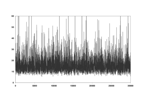
Figure 1: Markov chain paths for parameter $\nu_{1}^{(0)}$ of model $M_{0}$.

MCMC convergence. Figure 1 shows the first 30,000 samples, taken after the burn-in period, of the dof component $\nu^{(0)}_{1}$ for model $M_{0}$ (i.e. the case of the generalized $t$-copula). Since $M_{0}$ has the highest parameter dimensions among all the candidate models, in general it requires the longest length of chains to converge to a stationary distribution. This figure shows that after the burn-in period the samples are mixing well over the support of the posterior distribution.

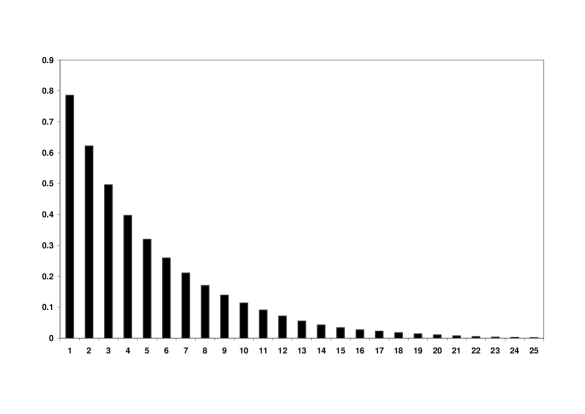
Figure 2: Autocorrelation of Markov chain samples for dof parameter $\nu_{1}^{(0)}$ of model $M_{0}$.

In addition to inspecting the sample paths, we also monitor the autocorrelation of the samples. Figure 2 shows the autocorrelations over multiple lags computed from the posterior samples for component $\nu^{(0)}_{1}$ of model $M_{0}$. A useful value to compute from these autocorrelations for each component is the autocorrelation time defined as

$$\tau_{k}=1+2\sum\limits_{g=1}^{\infty}{\rho_{k}(g)},$$ (26)

where $\rho_{k}(g)$ is the autocorrelation at lag $g$ for component $\theta_{k}$. This autocorrelation is sometimes used to compute an “effective sample size” by dividing the number of samples by $\tau_{k}$. The standard errors for the parameters can then be based on the effective sample size to compensate for the autocorrelation (see Ripley 1987, Neal 1993). In practice it is necessary to cut off the sum in (26) at $g=g_{k}^{\max}$ where the autocorrelations seem to have fallen to near zero, because including higher lags adds too much noise (for some interesting discussion on this issue, see Kass et al. 1998). As shown in Figure 2, in those well mixed MCMC samples the autocorrelation falls to near zero quickly and stays near zero at larger lags. For this study we have chosen a $g_{k}^{\max}$ for each component such that the autocorrelation at lag $g_{k}^{\max}$ has reduced to less than 0.01. That is, the autocorrelation time $\tau_{k}$ is estimated by

$$\hat{\tau}_{k}\approx 1+2\sum\limits_{g=1}^{g_{k}^{\max}}{\rho_{k}(g)},\quad g_{k}^{\max}=\min\{g:\rho_{k}(g)<0.01\}.$$ (27)

The $\hat{\tau}_{k}$ values estimated from MCMC output for model $M_{0}$ are shown in Table 2, along with the cut-off lag number $g_{k}^{\max}$. MCMC convergence characteristics for other components and for other models are very similar to those shown here for model $M_{0}$.

4.1 Bayesian estimates of parameters

This section presents results for posterior mean (MMSE), mode (MAP) and numerical error due to finite number of MCMC iterations.

4.1.1 Posterior mean and its numerical error

Table 3 shows values for the estimated mean from MCMC posterior samples for all 33 models. The standard errors (numerical error due to finite number of MCMC iterations) are shown in parentheses and the log-likelihoods corresponding to the estimated means are in the last column. Since the samples from MCMC are typically serially correlated, the usual formula for estimating the standard error of a sample mean (i.e. standard deviation divided by $\sqrt{N}$) will introduce significant under-estimation. Here, we use batch sampling for the standard error estimate of the MCMC posterior mean; see Gilks et al. (1996).

Consider a MCMC posterior sample $y_{1},y_{2},...,y_{N}$ with length $N=Q\times L$, where $L$ is sufficiently large, so that the batch means

$$\bar{y}_{q}=\frac{1}{L}\quad\sum\limits_{t=(q-1)L+1}^{q\times L}{\quad y^{(t)}\quad,\quad q=1,\dots,Q}$$ (28)

are considered approximately independent. Then $\bar{y}=(\bar{y}_{1}+\dots+\bar{y}_{Q})/Q$ and the standard error of the posterior sample mean $\bar{y}$ can be approximated by

$$\sqrt{\mathrm{Var}(\bar{y})}\approx\frac{1}{\sqrt{Q}}\sqrt{\frac{1}{Q-1}\quad\sum\limits_{q=1}^{Q}{(\bar{y}_{q}-\bar{y})^{2}}},$$ (29)

Note that $Q$ is the number of quasi-independent batches and $L=N/Q$ is the size of each batch.

4.1.2 Posterior mode and likelihood ratio tests

Values of the posterior mode taken from the MCMC samples for all the 33 models are shown in Table 4, along with the corresponding log-likelihood values. Using results of the maximum likelihood corresponding the posterior mode in Table 4, a classical likelihood ratio test can be performed to compare model likelihoods.

Consider the null hypothesis that the observed FX daily return data are from distribution described by the grouped $t$-copula model $M_{1}$, and the alternative hypothesis that the data are distributed according to the generalized $t$-copula model $M_{0}$. The likelihood ratio for the two models is simply $\Lambda=L_{1}/L_{0}$, where $L_{1}$ and $L_{0}$ are the maximum likelihood values (i.e. the likelihood value at the mode) for $M_{1}$ and $M_{0}$ respectively. The test statistic $-2\log(\Lambda)$ will be asymptotically $\chi^{2}$ distributed with degrees of freedom equal to the difference in the number of dof parameters in $M_{0}$ and $M_{1}$, which is 4 in this case.

We can perform likelihood ratio tests on all other grouped $t$-copula models ($\mbox{M}_{h},\;h=2,\dots,31$) against the same alternative hypothesis of model $M_{0}$, the generalized $t$-copula. For the standard $t$-copula the difference in the number of parameters is 5. The test statistic and the associated p-value ($\chi^{2}$ significance) are given in Table 4. Clearly, according to the p-value, all the null hypotheses should be rejected and the alternative hypothesis, the generalized $t$-copula model $M_{0}$, is statistically justified.

Excluding model $M_{0}$, among the other 32 $t$-copula models ($M_{h},\;h=1,\dots,32$), the one achieving the highest likelihood is $M_{27}$, which is one of the six (1,5) two-group configurations. The p-value of this best grouped $t$-copula model against $M_{0}$ is 0.0045 which is still very small, suggesting a rather strong rejection of the grouped $t$-copula (including the standard $t$-copula) in favour of the $\tilde{t}_{\rm{\bf\nu}}$-copula model $M_{0}$. Achieving the highest likelihood from the fifteen (2,4) configurations is model $M_{4}$. It is interesting to notice that both $M_{27}$ and $M_{4}$ have three European currencies (CHF, EUR, GBP) in one group (see Table 1), perhaps reflecting a natural geopolitical and economic grouping.

4.2 Bayesian model choice

While the likelihood ratio test relies on a single point estimate, the Bayesian model choice makes decisions based on the entire posterior distribution. As discussed in Section 3.3, three Bayesian inference criteria were used to choose among the 33 $t$-copula models: RISE given by (21); DIC given by (23); and the posterior model probabilities (24).

The RISE calculation involves fitting the MCMC posterior samples to a multivariate normal or $t$-distribution and taking expectation of the reciprocal likelihood. The DIC calculation requires taking expectation of the likelihood and the parameters. Column 2 in Table 5 shows the RISE factor $B_{0h}=R_{0}/R_{h},\;h=1,\dots,32$, where $R_{h}$ is the RISE value for model $M_{h}$. That is, $B_{0h}$ ($1\leq h\leq 32)$ is a measure of strength in the argument that the generalized $t$-copula (model $M_{0}$) is the Bayesian choice. The very large Bayes factors ($B_{0h}>e^{11}>5.9\times 10^{4})$ shown in Table 5 overwhelmingly support the generalized $t$-copula, confirming the likelihood ratio tests discussed previously. Excluding model $M_{0}$, these Bayes factors also point to $M_{27}$ as the most favoured model among the grouped $t$-copulas ($M_{h}$, $1\leq h\leq 32$) confirming the likelihood ratio tests. The larger the Bayes factor $B_{0h}$, the stronger the case against model $M_{h}$ ($1\leq h\leq 32)$.

The DIC values for 33 models are shown in column 3 of Table 5. Since only relative DIC value matters, the common constant in (22) was set in such a way that the DIC value for model $M_{0}$ is zero. As shown in Table 5, the DIC value for all the other models is significantly positive, relative to that of $M_{0}$. Thus under the DIC criterion the model of choice is clearly $M_{0}$, i.e. the generalized $t$-copula. In addition, similar to the RISE based Bayes factors and the likelihood tests, the DIC values also pick $M_{27}$ as the most likely grouped $t$-copula model after $M_{0}$, the same as the RISE factor and the likelihood ratio test. The larger the DIC value, the stronger the case against the model. It is interesting to observe that the magnitude of the DIC value is close to that of the logarithm of the Bayes factor based on the reciprocal importance sampling estimator, when both are evaluated relative to the same model $M_{0}$.

As shown by column 4 in Table 5, the results for posterior model probabilities (24) also agree with the RISE and DIC results, i.e. model $M_{0}$ has a very high probability of $88\%$, and model $M_{27}$ has the second highest probability. If we exclude model $M_{0}$, then model $M_{27}$ has a high probability of $68\%$. In summary, all three Bayesian choice criteria point to the same model $M_{0}$ as the best choice followed by model $M_{27}$, and these choices are in agreement with the classical likelihood ratio tests, as shown in Table 4.

5 Conditional Value-at-Risk

Consider a portfolio of six major currencies. Denote the exchange rates (USD per currency unit) for these currencies at time $t$ by $S_{i}^{(t)},\;i=1,\dots,6$. Assume we hold $\lambda_{i}$ units for the $i^{th}$ currency. The portfolio value at time $t$ is then $V^{(t)}=\sum\nolimits_{i=1}^{6}{\lambda_{i}S_{i}^{(t)}}$. The log-return for the $i^{th}$ currency at time $t+1$ is given by $x_{i}^{(t+1)}=\ln S_{i}^{(t+1)}-\ln S_{i}^{(t)}$. The portfolio loss for one time step is then

$$-\delta V^{(t+1)}=V^{(t)}-V^{(t+1)} = \sum\limits_{i=1}^{6}{\lambda_{i}S_{i}^{(t)}\left({1-\exp\left({x_{i}^{(t+1)}}\right)}\right)}$$ (30)

$$= V^{(t)}\sum\limits_{i=1}^{6}{w_{i}\left({1-\exp\left({x_{i}^{(t+1)}}\right)}\right)},$$

where $w_{i}=\lambda_{i}S_{i}^{(t)}/V^{(t)}$ is the proportion of the portfolio value in currency $i$ at time $t$, that is, it is the dollar weight of the $i^{th}$ currency. Now we wish to simulate the distribution of portfolio return

$$Z=-\delta V^{(t+1)}/V^{(t)}=\sum\limits_{i=1}^{6}{w_{i}\left({1-\exp\left({x_{i}^{(t+1)}}\right)}\right)}\approx\sum\limits_{i=1}^{6}{-w_{i}x_{i}^{(t+1)}}.$$

In the present study we model the dependence of the log-returns $x_{i}^{(t+1)}$ by one of the $t$-copula models as described in the previous sections. Recall that the dof parameters and their posterior distributions are already obtained by Bayesian MCMC. To focus on the impact of copula models, we use the standard normal distribution for all the six marginals. We take the CVaR as our risk measure. Assume that a random variable $Z$ has continuous density $f(\cdot)$ and distribution $F(\cdot)$. Given a threshold quantile level $\alpha$, the CVaR above $F^{-1}(\alpha)$ is defined as

$$CVaR_{\alpha}[Z]=E[Z|Z\geq F^{-1}(\alpha)]=\frac{1}{1-\alpha}{\kern 1.0pt}\,\int\limits_{F^{-1}(\alpha)}^{\infty}{xf(x)dx}{\kern 1.0pt},$$ (31)

which is the average of the losses exceeding $F^{-1}(\alpha)$. To demonstrate model impact on risk quantification, we compare CVaR of the two most likely models, $M_{0}$ and $M_{27}$, the best and the second best models of all 33 candidates. CVaR is calculated numerically using $10^{7}$ Monte Carlo simulations with $t$-copula model parameters given in Table (4).

Table 6 shows $CVaR_{0.99}^{(M_{0})}$ and $CVaR_{0.99}^{(M_{27})}$ predicted by models $M_{0}$ and $M_{27}$ for two portfolios (defined by weights in Table 6). Note in both portfolios we have negative weights (selling the currency) and the weights in each portfolio add to 1.0. As shown in Table 6, model $M_{27}$ underestimates the 0.99 CVaR by 16% for the first portfolio, and this underestimate reverses to a slight overestimate for the second portfolio, assuming the correct estimates are from model $M_{0}$. The second portfolio is only slightly different from the first – swapping the position of EUR and CHF (long/short position) in the first portfolio yields the second portfolio. The two portfolios are deliberately chosen to demonstrate that the model impact on risk quantification can be in either direction – it may be overestimation or it may be underestimation, depending on the portfolio. Thus it is important to choose the most suitable model statistically, such as by means of Bayesian model inference. Table 7 compares 0.99 CVaR prediction of model $M_{0}$ with that of model $M_{4}$, the most likely model from the (3,3) configuration, for the same two portfolios as those in Table 6. Here again the 0.99 CVaR for the first portfolio is underestimated by the incorrect model, and for the second portfolio it is overestimated.

6 Conclusion

This paper describes a Bayesian model choice methodology for $t$-copula models. As an illustration, altogether 33 $t$-copula models of six dimensions were considered: the generalized $t$-copula; the standard $t$-copula; and 31 grouped $t$-copula models from the complete subset of (3,3), (2,4) and (1,5) configurations. MCMC simulations under a Bayesian inference framework were performed to obtain the posterior distribution of dof parameters for all 33 $t$-copula models. Using historical data of foreign exchange rates as a case study, we found that Bayesian model choice based on the RISE, the DIC and the posterior model probabilities overwhelmingly favors the generalized $t$-copula model $M_{0}$. In addition, all three Bayesian choice criteria point to the same second most likely model $M_{27}$. These Bayesian choices are also in agreement with classical likelihood ratio tests.

The impact of model choice on the CVaR for two portfolios of six FX majors was observed to be significant.

For a comprehensive modeling of multivariate dependence in finance or insurance, there are other issues in data analysis that should be addressed carefully, such as time-dependent correlation parameters and validation. These are not considered in the present study.

7 Acknowledgement

We would like to thank Gareth Peters and John Donnelly for helpful discussions and comments on the manuscript.

Table 1: Group configurations and parameters for the 33 t-copula models.

Model	Group Configuration	Parameters
$\mbox{M}_{0}$	(AUD), (CAD), (CHF), (EUR), (GBP), (JPY)	$\nu_{1}^{(0)},\;\nu_{2}^{(0)},\;\nu_{3}^{(0)},\;\nu_{4}^{(0)},\;\nu_{5}^{(0)},\nu_{6}^{(0)}$
$\mbox{M}_{1}$	(AUD, CAD, CHF), (EUR, GBP, JPY)	$\nu_{1}^{(1)},\quad\nu_{2}^{(1)}$
$\mbox{M}_{2}$	(AUD, CAD, EUR), (CHF, GBP, JPY)	$\nu_{1}^{(2)},\quad\nu_{2}^{(2)}$
$\mbox{M}_{3}$	(AUD, CAD, GBP), (CHF, EUR, JPY)	$\nu_{1}^{(3)},\quad\nu_{2}^{(3)}$
$\mbox{M}_{4}$	(AUD, CAD, JPY), (CHF, EUR, GBP)	$\nu_{1}^{(4)},\quad\nu_{2}^{(4)}$
$\mbox{M}_{5}$	(AUD, CHF, EUR), (CAD, GBP, JPY)	$\nu_{1}^{(5)},\quad\nu_{2}^{(5)}$
$\mbox{M}_{6}$	(AUD, CHF, GBP), (CAD, EUR, JPY)	$\nu_{1}^{(6)},\quad\nu_{2}^{(6)}$
$\mbox{M}_{7}$	(AUD, CHF, JPY), (CAD, EUR, GBP)	$\nu_{1}^{(7)},\quad\nu_{2}^{(7)}$
$\mbox{M}_{8}$	(AUD, EUR, GBP), (CAD, CHF, JPY)	$\nu_{1}^{(8)},\quad\nu_{2}^{(8)}$
$\mbox{M}_{9}$	(AUD, EUR, JPY), (CAD, CHF, GBP)	$\nu_{1}^{(9)},\quad\nu_{2}^{(9)}$
$\mbox{M}_{10}$	(AUD, GBP, JPY), (CAD, CHF, EUR)	$\nu_{1}^{(10)},\quad\nu_{2}^{(10)}$
$\mbox{M}_{11}$	(GBP, JPY), (AUD, CAD, CHF, EUR)	$\nu_{1}^{(11)},\quad\nu_{2}^{(11)}$
$\mbox{M}_{12}$	(AUD, CAD), (CHF, EUR, GBP, JPY)	$\nu_{1}^{(12)},\quad\nu_{2}^{(12)}$
$\mbox{M}_{13}$	(AUD, CHF), (CAD, EUR, GBP, JPY)	$\nu_{1}^{(13)},\quad\nu_{2}^{(13)}$
$\mbox{M}_{14}$	(AUD, EUR), (CAD, CHF, GBP, JPY)	$\nu_{1}^{(14)},\quad\nu_{2}^{(14)}$
$\mbox{M}_{15}$	(AUD, GBP), (CAD, CHF, EUR, JPY)	$\nu_{1}^{(15)},\quad\nu_{2}^{(15)}$
$\mbox{M}_{16}$	(AUD, JPY), (CAD, CHF, EUR, GBP)	$\nu_{1}^{(16)},\quad\nu_{2}^{(16)}$
$\mbox{M}_{17}$	(CAD, CHF), (AUD, EUR, GBP, JPY)	$\nu_{1}^{(17)},\quad\nu_{2}^{(17)}$
$\mbox{M}_{18}$	(CAD, EUR), (AUD, CHF, GBP, JPY)	$\nu_{1}^{(18)},\quad\nu_{2}^{(18)}$
$\mbox{M}_{19}$	(CAD, GBP), (AUD, CHF, EUR, JPY)	$\nu_{1}^{(19)},\quad\nu_{2}^{(19)}$
$\mbox{M}_{20}$	(CAD, JPY), (AUD, CHF, EUR, GBP)	$\nu_{1}^{(20)},\quad\nu_{2}^{(20)}$
$\mbox{M}_{21}$	(CHF, EUR), (AUD, CAD, GBP, JPY)	$\nu_{1}^{(21)},\quad\nu_{2}^{(21)}$
$\mbox{M}_{22}$	(CHF, GBP), (AUD, CAD, EUR, JPY)	$\nu_{1}^{(22)},\quad\nu_{2}^{(22)}$
$\mbox{M}_{23}$	(CHF, JPY), (AUD, CAD, GBP, EUR)	$\nu_{1}^{(23)},\quad\nu_{2}^{(23)}$
$\mbox{M}_{24}$	(EUR, GBP), (AUD, CAD, CHF, JPY)	$\nu_{1}^{(24)},\quad\nu_{2}^{(24)}$
$\mbox{M}_{25}$	(EUR, JPY), (AUD, CAD, GBP, CHF)	$\nu_{1}^{(25)},\quad\nu_{2}^{(25)}$
$\mbox{M}_{26}$	(AUD), (CAD, CHF, EUR, GBP, JPY)	$\nu_{1}^{(26)},\quad\nu_{2}^{(26)}$
$\mbox{M}_{27}$	(CAD), (AUD, CHF, EUR, GBP, JPY)	$\nu_{1}^{(27)},\quad\nu_{2}^{(27)}$
$\mbox{M}_{28}$	(CHF), (CAD, AUD, EUR, GBP, JPY)	$\nu_{1}^{(28)},\quad\nu_{2}^{(28)}$
$\mbox{M}_{29}$	(EUR), (CAD, CHF, AUD, GBP, JPY)	$\nu_{1}^{(29)},\quad\nu_{2}^{(29)}$
$\mbox{M}_{30}$	(GBP), (CAD, CHF, EUR, AUD, JPY)	$\nu_{1}^{(30)},\quad\nu_{2}^{(30)}$
$\mbox{M}_{31}$	(JPY), (CAD, CHF, EUR, GBP, AUD)	$\nu_{1}^{(31)},\quad\nu_{2}^{(31)}$
$\mbox{M}_{32}$	(AUD, CAD, CHF, EUR, GBP, JPY)	$\nu_{1}^{(32)}$

Table 2: Autocorrelation estimates and corresponding cut-off lag number.

Parameter	$\nu_{1}^{(0)}$	$\nu_{2}^{(0)}$	$\nu_{3}^{(0)}$	$\nu_{4}^{(0)}$	$\nu_{5}^{(0)}$	$\nu_{6}^{(0)}$
$\hat{\tau}_{k}$	8.79	2.23	23.5	23.1	8.41	8.69
$g_{k}^{\max}$	23	14	65	57	30	34

Table 3: MCMC output values of posterior mean, standard error and log-likelihood.

Model	Posterior Mean (Standard Error)	Log-likelihood
$M_{0}$	$\nu_{1}^{(0)}=15.4(0.79)$,  $\nu_{2}^{(0)}=67.3(1.3)$,  $\nu_{3}^{(0)}=8.76(0.34)$,	2353.1
	$\nu_{4}^{(0)}=6.38(0.20)$,  $\nu_{5}^{(0)}=11.6(0.46)$, $\nu_{6}^{(0)}=18.3(1.1)$
$M_{1}$	$\nu_{1}^{(1)}=15.1\;(0.29),\quad\nu_{2}^{(1)}=9.37\;(0.14)$	2342.8
$M_{2}$	$\nu_{1}^{(2)}=10.2\;(0.15),\quad\nu_{2}^{(2)}=13.4\;(0.21)$	2338.6
$M_{3}$	$\nu_{1}^{(3)}=18.2\;(0.28),\quad\nu_{2}^{(3)}=8.56\;(0.09)$	2341.9
$M_{4}$	$\nu_{1}^{(4)}=24.4\;(0.82),\quad\nu_{2}^{(4)}=7.78\;(0.16)$	2343.8
$M_{5}$	$\nu_{1}^{(5)}=8.51\;(0.13),\quad\nu_{2}^{(5)}=18.7\;(0.49)$	2341.9
$M_{6}$	$\nu_{1}^{(6)}=13.4\;(0.26),\quad\nu_{2}^{(6)}=10.2\;(0.16)$	2338.6
$M_{7}$	$\nu_{1}^{(7)}=13.6\;(0.27),\quad\nu_{2}^{(7)}=10.3\;(0.17)$	2338.6
$M_{8}$	$\nu_{1}^{(8)}=9.24(0.13),\quad\nu_{2}^{(8)}=15.7\;(0.35)$	2343.2
$M_{9}$	$\nu_{1}^{(9)}=8.76(0.13),\quad\nu_{2}^{(9)}=14.0\;(0.32)$	2343.2
$M_{10}$	$\nu_{1}^{(10)}=12.6(0.23),\quad\nu_{2}^{(10)}=11.1\;(0.17)$	2336.7
$M_{11}$	$\nu_{1}^{(11)}=27.9(4.87),\quad\nu_{2}^{(11)}=8.6\;(0.09)$	2336.7
$M_{12}$	$\nu_{1}^{(12)}=14.1(0.44),\quad\nu_{2}^{(12)}=10.6\;(0.14)$	2336.7
$M_{13}$	$\nu_{1}^{(13)}=8.56(0.11),\quad\nu_{2}^{(13)}=13.8\;(0.25)$	2343.6
$M_{14}$	$\nu_{1}^{(14)}=13.2(0.74),\quad\nu_{2}^{(14)}=11.1\;(0.14)$	2336.7
$M_{15}$	$\nu_{1}^{(15)}=13.3(0.94),\quad\nu_{2}^{(15)}=11.2\;(0.17)$	2336.6
$M_{16}$	$\nu_{1}^{(16)}=17.4(0.85),\quad\nu_{2}^{(16)}=9.78\;(0.13)$	2343.0
$M_{17}$	$\nu_{1}^{(17)}=9.78(0.14),\quad\nu_{2}^{(17)}=12.9\;(0.2)$	2338.9
$M_{18}$	$\nu_{1}^{(18)}=24.9(4.4),\quad\nu_{2}^{(18)}=8.96\;(0.09)$	2342.5
$M_{19}$	$\nu_{1}^{(19)}=32.5(7.99),\quad\nu_{2}^{(19)}=8.76\;(0.08)$	2343.4
$M_{20}$	$\nu_{1}^{(20)}=7.46(0.11),\quad\nu_{2}^{(20)}=16.8\;(0.59)$	2343.0
$M_{21}$	$\nu_{1}^{(21)}=14.2(0.43),\quad\nu_{2}^{(21)}=10.5\;(0.14)$	2338.6
$M_{22}$	$\nu_{1}^{(22)}=14.3(0.49),\quad\nu_{2}^{(22)}=10.5\;(0.15)$	2338.4
$M_{23}$	$\nu_{1}^{(23)}=8.64(0.11),\quad\nu_{2}^{(23)}=14.2\;(0.32)$	2343.7
$M_{24}$	$\nu_{1}^{(24)}=8.66(0.09),\quad\nu_{2}^{(24)}=13.6\;(0.23)$	2343.4
$M_{25}$	$\nu_{1}^{(25)}=12.8(0.50),\quad\nu_{2}^{(25)}=11.2\;(0.13)$	2336.7
$M_{26}$	$\nu_{1}^{(26)}=15.2(1.63),\quad\nu_{2}^{(26)}=11.3\;(0.31)$	2336.4
$M_{27}$	$\nu_{1}^{(27)}=64.7(3.01),\quad\nu_{2}^{(27)}=9.26\;(0.24)$	2346.7
$M_{28}$	$\nu_{1}^{(28)}=16.0(1.15),\quad\nu_{2}^{(28)}=11.0\;(0.38)$	2338.4
$M_{29}$	$\nu_{1}^{(29)}=7.94(0.32),\quad\nu_{2}^{(29)}=12.9\;(0.48)$	2344.4
$M_{30}$	$\nu_{1}^{(30)}=15.1(1.53),\quad\nu_{2}^{(30)}=11.3\;(0.32)$	2336.5
$M_{31}$	$\nu_{1}^{(31)}=11.4(0.32),\quad\nu_{2}^{(31)}=1.81\;(0.17)$	2336.4
$M_{32}$	$\nu_{1}^{(32)}=11.4\;(0.14)$	2336.8

Table 4: MCMC output values of posterior mode, corresponding log-likelihood, likelihood ratio $\Lambda$ and p-value comparing $M_{h}$ with $M_{0}$.

Model	MCMC posterior mode	Log-likelihood	$-2\log(\Lambda)$	p-value
$M_{0}$	${\bm{\nu}}^{(0)}=(11.5,82.4,7.92,5.81,10.3,14.3)$	2354.3	0	N/A
$M_{1}$	${\bm{\nu}}^{(1)}=(14.0,\quad 8.96)$	2342.9	22.8	0.00014
$M_{2}$	${\bm{\nu}}^{(2)}=(9.75,\quad 12.6)$	2338.7	31.2	$<$0.00001
$M_{3}$	${\bm{\nu}}^{(3)}=(16.6,\quad 8.22)$	2342.1	24.4	$<$0.0001
$M_{4}$	${\bm{\nu}}^{(4)}=(21.0,\quad 7.49)$	2344.1	20.4	0.00042
$M_{5}$	${\bm{\nu}}^{(5)}=(8.17,\quad 16.9)$	2342.1	24.4	$<$0.0001
$M_{6}$	${\bm{\nu}}^{(6)}=(12.6,\quad 9.73)$	2338.8	31.0	$<$0.00001
$M_{7}$	${\bm{\nu}}^{(7)}=(12.8,\quad 9.79)$	2338.7	31.2	$<$0.00001
$M_{8}$	${\bm{\nu}}^{(8)}=(8.84,\quad 14.4)$	2343.4	21.8	0.00022
$M_{9}$	${\bm{\nu}}^{(9)}=(8.76,\quad 14.0)$	2343.3	22.0	0.00020
$M_{10}$	${\bm{\nu}}^{(10)}=(11.8,\quad 10.5)$	2336.9	34.8	$<$0.000001
$M_{11}$	${\bm{\nu}}^{(11)}=(22.6,\quad 8.68)$	2343.0	22.6	0.00015
$M_{12}$	${\bm{\nu}}^{(12)}=(13.1,\quad 10.2)$	2338.6	31.5	$<$0.00001
$M_{13}$	${\bm{\nu}}^{(13)}=(8.23,\quad 13.1)$	2343.7	21.3	0.00028
$M_{14}$	${\bm{\nu}}^{(14)}=(11.9,\quad 10.7)$	2336.9	34.8	$<$0.000001
$M_{15}$	${\bm{\nu}}^{(15)}=(11.7,\quad 10.8)$	2336.8	34.9	$<$0.000001
$M_{16}$	${\bm{\nu}}^{(16)}=(15.7,\quad 9.39)$	2343.2	22.2	0.00018
$M_{17}$	${\bm{\nu}}^{(17)}=(9.31,\quad 12.7)$	2339.0	30.6	$<$0.00001
$M_{18}$	${\bm{\nu}}^{(18)}=(20.9,\quad 8.66)$	2342.7	23.1	0.00012
$M_{19}$	${\bm{\nu}}^{(19)}=(25.2,\quad 8.48)$	2343.8	21.1	0.00030
$M_{20}$	${\bm{\nu}}^{(20)}=(7.14,\quad 15.7)$	2343.1	22.3	0.00017
$M_{21}$	${\bm{\nu}}^{(21)}=(13.2,\quad 10.1)$	2338.5	31.5	$<$0.00001
$M_{22}$	${\bm{\nu}}^{(22)}=(13.3,\quad 10.1)$	2338.5	31.5	$<$0.00001
$M_{23}$	${\bm{\nu}}^{(23)}=(8.27,\quad 13.4)$	2343.8	21.0	0.00031
$M_{24}$	${\bm{\nu}}^{(24)}=(8.31,\quad 12.9)$	2343.5	21.7	0.00023
$M_{25}$	${\bm{\nu}}^{(25)}=(11.7,\quad 10.8)$	2336.8	34.9	$<$0.000001
$M_{26}$	${\bm{\nu}}^{(26)}=(11.8,\quad 10.9)$	2336.8	34.9	$<$0.000001
$M_{27}$	${\bm{\nu}}^{(27)}=(68.3,\quad 9.03)$	2346.8	15.1	0.0045
$M_{28}$	${\bm{\nu}}^{(28)}=(14.0,\quad 10.5)$	2338.6	31.4	$<$0.00001
$M_{29}$	${\bm{\nu}}^{(29)}=(7.55,\quad 12.2)$	2344.5	19.6	0.00060
$M_{30}$	${\bm{\nu}}^{(30)}=(12.0,\quad 10.9)$	2336.8	34.9	$<$0.000001
$M_{31}$	${\bm{\nu}}^{(31)}=(11.4,\quad 11.0)$	2336.8	35.0	$<$0.000001
$M_{32}$	${\bm{\nu}}^{(32)}=(11.1)$	2336.9	34.9	$<$0.00001

Table 5: Bayes factors $B_{0i}$, DIC and model probabilities of all candidates.

Model	Log($B_{0h}$)	DIC	Model prob. $(\%)$	Model prob. $(\%)$ excl. $M_{0}$
$M_{0}$	0	0	88.5	N/A
$M_{1}$	16.7	15.8	0.15	1.28
$M_{2}$	20.1	24.0	$<0.1$	$<0.1$
$M_{3}$	16.6	17.5	$<0.1$	0.54
$M_{4}$	16.4	13.0	0.45	3.89
$M_{5}$	18.7	17.4	$<0.1$	0.55
$M_{6}$	19.3	24.1	$<0.1$	$<0.1$
$M_{7}$	21.5	24.3	$<0.1$	$<0.1$
$M_{8}$	14.5	15.0	0.12	1.07
$M_{9}$	18.9	15.1	0.22	1.89
$M_{10}$	21.9	27.8	$<0.1$	$<0.1$
$M_{11}$	18.0	15.6	0.15	1.26
$M_{12}$	24.9	24.7	$<0.1$	$<0.1$
$M_{13}$	14.9	14.3	0.31	2.68
$M_{14}$	23.2	27.9	$<0.1$	$<0.1$
$M_{15}$	25.5	28.0	$<0.1$	$<0.1$
$M_{16}$	14.2	15.3	0.20	1.73
$M_{17}$	21.7	23.7	$<0.1$	$<0.1$
$M_{18}$	15.3	16.1	0.12	1.03
$M_{19}$	15.1	14.1	0.29	2.52
$M_{20}$	15.1	15.3	0.19	1.64
$M_{21}$	21.5	24.3	$<0.1$	$<0.1$
$M_{22}$	20.6	24.6	$<0.1$	$<0.1$
$M_{23}$	17.1	14.1	0.36	3.10
$M_{24}$	15.4	14.7	0.25	2.22
$M_{25}$	22.6	27.9	$<0.1$	$<0.1$
$M_{26}$	22.2	28.0	$<0.1$	$<0.1$
$M_{27}$	11.0	6.73	7.8	68.3
$M_{28}$	21.0	24.6	$<0.1$	$<0.1$
$M_{29}$	16.3	12.7	0.7	6.18
$M_{30}$	28.0	28.0	$<0.1$	$<0.1$
$M_{31}$	22.8	28.1	$<0.1$	$<0.1$
$M_{32}$	22.3	28.1	$<0.1$	$<0.1$

Table 6: The 0.99 conditional Value-at-Risk ($CVaR_{0.99}$) predicted by model $M_{0}$ and $M_{27}$, for two portfolios of six major currencies. $\delta=(CVaR_{0.99}^{M_{27}}-CVaR_{0.99}^{M_{0}})/CVaR_{0.99}^{M_{0}}$ is the relative difference of CVaR between $M_{27}$ and $M_{0}$. Standard errors are in parentheses.

Portfolio asset weights $w_{i}$	$CVaR_{0.99}^{(M_{0})}$	$CVaR_{0.99}^{(M_{27})}$	$\delta$
(AUD, CAD, CHF, EUR, GBP, JPY)
(0.25, 0.25, 0.8, -0.8, 0.25, 0.25)	1.707 (0.004)	1.425 (0.003)	-16.5%
(0.25, 0.25, -0.8, 0.8, 0.25, 0.25)	1.737 (0.003)	1.782 (0.003)	2.6%

Table 7: The 0.99 conditional Value-at-Risk ($CVaR_{0.99}$) predicted by model $M_{0}$ and $M_{4}$, for two portfolios of six major currencies. $\delta=(CVaR_{0.99}^{M_{4}}-CVaR_{0.99}^{M_{0}})/CVaR_{0.99}^{M_{0}}$ is the relative difference of CVaR between $M_{4}$ and $M_{0}$. Standard errors are in parentheses.

Portfolio asset weights $w_{i}$	$CVaR_{0.99}^{(M_{0})}$	$CVaR_{0.99}^{(M_{4})}$	$\delta$
(AUD, CAD, CHF, EUR, GBP, JPY)
(0.25, 0.25, 0.8, -0.8, 0.25, 0.25)	1.571 (0.004)	1.366 (0.003)	-13.0%
(0.25, 0.25, -0.8, 0.8, 0.25, 0.25)	1.608 (0.003)	1.732 (0.003)	7.7%

References

- [1] Berger, J. O. (1985) Statistical Decision Theory and Bayesian Analysis. Springer-Verlag, New York.
- [2] Breymann, W., Dias, A. and Embrechts, P. (2003) Dependence structures for multivariate high-frequency data in finance. Quantitative Finance 3, 1–14.
- [3] Cairns, A. (2000) A discussion of of parameter and model uncertainty in insurance. Insurance: Mathematics and Economics 27, 313–330.
- [4] Chib, S. (1995) Marginal likelihood from the Gibbs output. Journal of the American Statistical Association 90(432), 1313–1321.
- [5] Congdon, P. (2006) Bayesian Statistical Modelling. John Wiley & Sons, Ltd, 2nd edn.
- [6] Daul, S., De Giorgi, E., Lindskog, F. and McNeil, A. (2003) The grouped t-copula with an application to credit risk. Risk 16, 73–76.
- [7] Demarta, S. and McNeil, A. (2005) The t copula and related copulas. International Statistical Review 73(1), 111–129.
- [8] Embrechts, P., McNeil, A. and Straumann, D. (2001) Correlation and dependence in risk management: properties and pitfalls. Dempster, M. and Moffatt, H. (Eds.), Risk Management: Value at Risk and Beyond, pp. 176–223, Cambridge University Press.
- [9] Fang, H., Fang, K. and Kotz, S. (2002) The meta-elliptical distributions with given marginals. Journal of Multivariate Analysis 82, 1–16.
- [10] Fruhwirth-Schnatter, S. (1995) Bayesian model discrimination and bayes factor for linear Gaussian state space models. Journal of the Royal Statistical Society, series B 57, 237–246.
- [11] Fruhwirth-Schnatter, S. (2004) Estimating marginal likelihoods for mixture and markov switching models using bridge sampling techniques. The Econometrics Journal 7, 143–167.
- [12] Gelfand, A. and Dey, D. (1994) Bayesian model choice: Asymptotic and exact calculations. Journal of the Royal Statistical Society, series B 56, 501–514.
- [13] Gelfand, A. and Smith, A. (1990) Sampling-based approaches to calculating marginal densities. Journal of the American Statistical Association 85, 398–409.
- [14] Gelman, A., Gilks, W. R. and Roberts, G. O. (1997) Weak convergence and optimal scaling of random walk Metropolis algorithm. Annals of Applied Probability 7, 110–120.
- [15] Gilks, W. R., Richardson, S. and Spiegelhalter, D. J. (1996) Markov Chain Monte Carlo in practice. Chapman & Hall, London.
- [16] Green, P. (1995) Reversible jump MCMC computation and Bayesian model determination. Biometrika 82, 711–732.
- [17] Hastings, W. (1970) Monte Carlo sampling methods using Markov chains and their applications. Biometrika 57, 97–109.
- [18] Jeffreys, H. (1961) Theory of Probability. Oxford University Press, Oxford, 3 edn.
- [19] Joe, H. (1997) Multivariate Models and Dependence Concepts. Chapman & Hall, London.
- [20] Kass, R. and Raftery, A. (1995) Bayes factor. Journal of the American Statistical Association 90, 773–792.
- [21] Kass, R. E., Carlin, B. P., Gelman, A. and Neal, R. M. (1998) Markov chain Monte Carlo in practice: a roundtable discussion. The American Statistician 52(2), 93–100.
- [22] Lavine, M. and Schervish, M. J. (1999) Bayes factors: what they are and what they are not. The American Statistician 53(2), 119–122.
- [23] Luo, X. and Shevchenko, P. V. (2010) The t copula with multiple parameters of degrees of freedom: bivariate characteristics and application to risk management. Quantitative Finance 10(9), 1039–1054.
- [24] Luo, X. and Shevchenko, P. V. (2010) LGD credit risk model: estimation of capital with parameter uncertainty using MCMC. Preprint arXiv:1011.2827v3 available from http://arxiv.org.
- [25] Mashal, R., Naldi, M. and Zeevi, A. (2003) On the dependence of equity and asset returns. Risk 16, 83–87.
- [26] McNeil, A. J., Frey, R. and Embrechts, P. (2005) Quantitative Risk Management: Concepts, Techniques and Tools. Princeton University Press, Princeton.
- [27] Meng, X. and Wong, W. (1996) Simulating ratios of normalizing constants via a simple identity. Statistical Sinica 6, 831–860.
- [28] Metropolis, N., Rosenbluth, A. W., Rosenbluth, M. N., Teller, A. H. and Teller, E. (1953) Equations of state calculations by fast computing machines. Journal of Chemical physics 21, 1087–1091.
- [29] Miazhynskaia, T. and Dorffner, G. (2006) A comparison of Bayesian model selection based on MCMC with an application to GARCH-type models. Statistical Papers 47, 525–549.
- [30] Neal, R. M. (1993) Porbabilistic inference using Markov chain samplers. Technical report, Department of Computer Science, University of Toronto.
- [31] Newton, M. and Raftery, A. (1994) Approximate Bayesian inference by the weighted likelihood bootstrap. Journal of the Royal Statistical Society, series B 56, 1–48.
- [32] Peters, G. W., Shevchenko, P. V. and Wüthrich, M. V. (2009) Model uncertainty in claims reserving within Tweedie’s compound poisson models. ASTIN Bulletin 39(1), 1–33.
- [33] Peters, G. W., Wüthrich, M. V. and Shevchenko, P. V. (2010) Chain ladder method: Bayesian bootstrap versus classical bootstrap. Insurance Mathematics and Economics 47(1), 36–51.
- [34] Piessens, R., De Doncker-Kapenga, E., Überhuber, C. W. and Kahaner, D. K. (1983) QUADPACK – a Subroutine Package for Automatic Integration. Springer-Verlag.
- [35] Ripley, B. D. (1987) Stochastic Simulation. Wiley, New York.
- [36] Robert, C. P. (2001) The Bayesian Choice. Springer Verlag, New York.
- [37] Roberts, G. O. and Rosenthal, J. S. (2001) Optimal scaling for various Metropolis-Hastings algorithms. Statistical Science 16, 351–367.
- [38] Schwarz, G. (1978) Estimation the dimension of a model. Annals of Statistics 6, 461–464.
- [39] Shevchenko, P. V. (2010) Implementing loss distribution approach for operational risk. Applied Stochastic Models in Business and Industry 26(3), 277–307.
- [40] Sklar, A. (1959) Fonctions de r partition n dimensions et leurs marges. Publ. Inst. Statist. Univ. Paris 8, 229–231.
- [41] Spiegelhalter, D. J., Best, N. G., Carlin, B. P. and Van Der Linde, A. (2002) Bayesian measures of model complexity and fit. Journal of the Royal Statistical Society: Series B 64(4), 583–639.
- [42] Tanner, M. A. and Wong, W. H. (1987) The calculation of posterior distributions by data augmentation. Journal of American Statistical Association 82(398), 528–540.
- [43] Venter, G., Barnett, J., Kreps, R. and Major, J. (2007) Multivariate copulas for financial modeling. Variance 1(1), 103–119.
- [44] Wasserman, L. (1997) Bayesian model selection and model averaging. Technical report, Statistics Department, Carnegie Mellon University.