A multistep algorithm for ODEs

Abstract

The objective of this paper is to prove the convergence of a linear implicit multi-step numerical method for ordinary differential equations. The algorithm is obtained via Taylor approximations. The convergence is proved following the Dahlquist theory. As an additional topic, the time stability is established too. Comparative tests between some of the most known numerical methods and this method are presented.

Keywords Taylor approximation, multi-step method, stability, consistency, time regions stability.

AMS (MOS) subject classification: 65L06, 65P99.

1 Introduction

We present a linear implicit m-step method LIL (Local Iterative Linearization) and prove its convergence applied for the following initial value problem

$$\overset{.}{x}=f\,(t,x),\quad x(t_{0})=x_{0},$$ (1)

where  $f\,:\,[t_{0},T]\times\mathbb{R}^{n}\rightarrow\mathbb{R}^{n}$, $T>0,\,t_{0}\in\mathbb{R}_{+},$ is a $C^{\,m}$ smooth Lipschitz function.

Although the classical linear multi-step algorithms are very known and utilized, the LIL characteristics (convergence properties, time stability and applications results) show that this numerical method could be considered as an interesting alternative to the widely used formulas.

The backward approximation of derivatives implies null coefficients of the odd order derivatives which represent a major advantage for the propagation of errors.

As a comparative test two simple ODEs with known analytical solutions and a chaotic continuous-time dynamical system, first studied by Fabrikant and Rabinovich [6] and recent numerically re-examined by Danca and Chen [3], was integrated using the LIL algorithm and some of the most known algorithms. The complex dynamic of this special model represented a real challenge for almost all of these methods as shown in Sect.5.

Being an implicit method, an extrapolation is used as the predictor phase. Like all the $m$-step algorithms, the previous  $m$  points (beside the first  $m$  start points) should be estimated every step.

To study the convergence we use the unified approach of stability and consistency developed by Germund Dahlquist in 1956 [2] (see also [7-8]). Thus, the LIL method applied to the initial value problem (1) is considered convergent if and only if it is stable and consistent.

The content of this paper is as follows: In Sect. 2 the LIL method is deduced. The convergence is proved in Sect. 3. In Sect. 4 is presented the time stability with the corresponding time stability domains. In Sect. 5 three examples are presented. All computer tests were realized using a Turbo Pascal code written by the author. In the Appendix, the coefficients of LIL method are presented.

2 Deduction of the LIL method

Let us consider the uniform grid

$$\Delta=(t_{0}<t_{1}<...<t_{n}=T\,),\quad n\in\mathbb{N}^{\ast},$$

with the step-size

$$h=\frac{T-t_{0}}{n}=2\,\delta t\,,$$

where  $\delta t$  stands for the ray of the neighborhood  $V_{k}=\left(t_{k}-\delta t\,,\,t_{k}+\delta t\right)\,,$  $k=1,2,...,n-1.$

We assume that all infinite Taylor series converge, but this is not necessarily since one truncate at a sufficiently large but finite number of terms.

One introduce the following notations

$$x_{k-j} : =x(t_{k-j})=x\left[t_{0}+\left(k-j)h\right)\right],$$

$$x_{k}^{(i)} : =x^{(i)}(t_{k}),\quad x_{k}^{(0)}:=x(t_{k}),\quad\qquad j=1,2,...,m.$$

In the following  $k$  is supposed to take the values  $k=1,2,...,n-1.$

If we consider  $x_{k-j}$  as a function of variable $h$  defined in  $V_{k}$ , then the first  $m$  terms of Taylor approximation of  $x_{k-j}$  is

$$x_{k-j}\thickapprox x_{k}-\frac{j\,h}{1!}x_{k}^{{}^{\prime}}+\frac{\left(j\,h\right)^{2}}{2!}x_{k}^{{}^{\prime\prime}}-...+\left(-1\right)^{m}\frac{\left(j\,h\right)^{m}}{m!}x_{k}^{\left(m\right)},$$ (2)

where  $j=1,2,...m.$  The relations  (2) represent a Cramer system with the unknown  $x_{k}^{\left(i\right)},\ i=1,2,...,m$

$$\begin{array}[t]{l}x_{k-1}-x_{k}\thickapprox\frac{h}{1!}x_{k}^{{}^{\prime}}+\frac{\,h^{2}}{2!}x_{k}^{{}^{\prime\prime}}-...+\left(-1\right)^{m}\frac{\,h^{m}}{m!}x_{k}^{\left(m\right)},\\ x_{k-2}-x_{k}\thickapprox\frac{2\,h}{1!}x_{k}^{{}^{\prime}}+\frac{\left(2\,h\right)^{2}}{2!}x_{k}^{{}^{\prime\prime}}-...+\left(-1\right)^{m}\frac{\left(2\,h\right)^{m}}{m!}x_{k}^{\left(m\right)},\\ ...\\ x_{k-m}-x_{k}\thickapprox\frac{m\,h}{1!}x_{k}^{{}^{\prime}}+\frac{\left(m\,h\right)^{2}}{2!}x_{k}^{{}^{\prime\prime}}-...+\left(-1\right)^{m}\frac{\left(m\,h\right)^{m}}{m!}x_{k}^{\left(m\right)}.\end{array}$$ (3)

The determinant of the system (3) is

$$\Delta=\frac{h^{{}^{m\left(m+1\right)/2}}}{1!2!...m!}\left|\begin{array}[]{lllll}1&1&1&...&1\\ 2&2^{2}&2^{3}&...&2^{m}\\ ...&...&...&...&...\\ m&m^{2}&m^{3}&...&m^{m}\end{array}\right|=h^{{}^{{}^{m\left(m+1\right)/2}}}1!2!...\left(m-2\right)!\,.$$

Because for  $m\geq 2$  we have $\,\Delta\neq 0$,  there exists a unique solution

$$x_{k}^{\left(i\right)} = \frac{1}{h^{i}}\sum_{j=0}^{m}\delta_{i\,j}x_{k-j},\quad i=2,...,m\quad\text{for \ \ }m\geq i>1,$$

$$x_{k}^{{}^{\prime}} = \frac{x_{k}-x_{k-1}}{h}\quad\text{for \ }m=i=1,$$

the coefficients  $\delta_{i\,j}$  being drawn in Table 7/Appendix.

Thus we obtained a backward approximation of derivatives, which represents the key of LIL method. The Taylor approximation of the solution  $x$, considered now as function of  $t$  in the neighborhood  $V_{k},$  is

$$x(t)\thickapprox x(t_{k})+\frac{t-t_{k}}{1!}x^{{}^{\prime}}(t_{k})+\frac{\left(t-t_{k}\right)^{2}}{2!}x^{{}^{\prime\prime}}(t_{k})+...+\frac{\left(t-t_{k}\right)^{m}}{m!}x^{\left(m\right)}(t_{k}).$$ (4)

Next, integrating (4) in $\ V_{k}$  we get

$$\begin{array}[]{l}\int\limits_{t_{k}-\delta\,t}^{t_{k}+\delta\,t}x(t)\,dt=\int\limits_{-\,\delta\,t}^{\delta\,t}x(t+t_{k})\,dt\thickapprox\int\limits_{-\,\delta\,t}^{\delta\,t}\left(\sum\limits_{i\,=0}^{m}x_{k}^{\left(i\right)}t^{i}\right)dt=\\ =\sum\limits_{\begin{subarray}{c}i\,=0,2,4,...\\ i\leq\,m\end{subarray}}^{m}\frac{1}{2^{i}\left(i+1\right)!}h^{i+1}x_{k}^{\left(i\right)}=h\,x_{k}+h^{3}\frac{1}{24}x_{k}^{{}^{\prime\prime}}+h^{5}\frac{1}{1920}x_{k}^{\left(4\right)}+...\end{array}$$ (5)

Remark 1

The zero coefficients of the derivatives  $x_{k}^{\left(2i+1\right)}$  for $\,i=0,1,2,...$ in (5) represent a major advantage for the propagation of errors and computation time.

If we use in (5) the derivatives expression (2.3) we have

$$\int\limits_{t_{k}-\delta\,t}^{t_{k}+\delta\,t}x(t)\,dt\thickapprox h\sum_{i=0}^{m}\sigma_{0\,i}x_{k-i}\,$$ (6)

the coefficients  $\sigma_{0\,i}$  being given in Table 8(a)/Appendix. Using the same way one can approximate  $x^{\prime}$  on  $V_{k}$

$$\int\limits_{t_{k}-\delta\,t}^{t_{k}+\delta\,t}x^{\prime}(t)\,dt\thickapprox\sum_{i=0}^{m}\sigma_{1\,i}x_{k-i}\,,$$ (7)

the coefficients  $\sigma_{1i}$  being drawn in Table 8(b)/Appendix.

To overcome the difficulty of Taylor approximation of the composite function  $f$  we found, empirically, that the relations (6) could be considered as a simple way to approximate the integral of  $f$  without altering the method convergence. Thus

$$\int\limits_{t_{k}-\delta\,t}^{t_{k}+\delta\,t}f\,(t,x(t))\,dt\thickapprox h\sum_{i\,=\,0}^{m}\sigma_{0\,i}\,\,f_{k-i},$$ (8)

where  $f_{k-i}:=f\,(t_{k-i},x(t_{k-i}))$ .

Using (7) and (8) we can integrate (1) in  $V_{k}\,$

$$\sum_{i\,=\,0}^{m}\sigma_{1i}x_{k-i}=h\,\sum_{i\,=\,0}^{m}\sigma_{0\,i}\,\,f_{k-i}\,.$$

Because  $\sigma_{10}\neq 0$ ,  for every  $m\,\$(see Table 8/Appendix),  the approximation of the solution in  $V_{k}$  is

$$x_{k}=\frac{\,h}{\sigma_{10}}\sum\limits_{i\,=\,0}^{m}\sigma_{0\,i}\,\,f_{k-i}-\frac{1}{\sigma_{10}}\sum\limits_{i\,=\,1}^{m}\sigma_{1\,i}\,x_{k-i}.$$ (9)

If we denote

$$u_{k}:=\frac{\,1}{\sigma_{10}}\sum\limits_{i\,=\,0}^{m}\sigma_{0\,i}\,\,f_{k-i},\quad v_{k}:=-\,\frac{1}{\sigma_{10}}\sum\limits_{i\,=\,1}^{m}\sigma_{1\,i}\,x_{k-i},$$

the relations (9) become

$$x_{k}=v_{k}+h\,u_{k}\,,\quad k=1,2,...n-1\,.$$ (10)

Formula (10) represents the $m\,$th-order LIL method. In Table 1 the formulae for orders one through five ($m\in\{1,2,3,4,5\})$ are presented.

$m$
$1$	$x_{k}=x_{k-1}+h\,f_{k},$
$2$	$x_{k}=\frac{4}{3}x_{k-1}-\frac{1}{3}x_{k-2}+\frac{h}{36}\left(25\,f_{k}-2\,f_{k-1}+f_{k-2}\right),$
$3$	$x_{k}=\frac{5}{3}x_{k-1}-\frac{13}{15}x_{k-2}+\frac{1}{5}x_{k-3}+\frac{h}{45}\left(26\,f_{k}-5\,f_{k-1}+4\,f_{k-2}-f_{k-3}\right)$
$4$	$x_{k}=2x_{k-1}-\frac{8}{5}x_{k-2}+\frac{26}{35}x_{k-3}-\frac{1}{7}x_{k-4}+\frac{h}{12600}(6463\,f_{k}-2092f_{k-1}$
	$\,\,\,\,\,\,\,\,\,\,\,+2298f_{k-2}-1132f_{k-3}+223f_{k-4}),$
$5$	$x_{k}=\frac{7}{3}x_{k-1}-\frac{38}{15}x_{k-2}+\frac{62}{35}x_{k-3}-\frac{43}{63}x_{{k-4}}+\frac{1}{9}x_{k-5}+\frac{h}{14175}(6669\,f_{k}$
	$\,\,\,\,\,\,\,\,\,\,\,-3122\,f_{k-1}+4358\,f_{k-2}-3192\,\,f_{k-3}+1253\,\,f_{k-4}-206\,f_{k-5}).$

Table 1: LIL algorithms.

The study was achieved up to  $m=8,$  but in this paper for the sake of simplicity we considered only  $m\in\{1,2,3,4,5\}$. For  $m=1$ the LIL method is equivalent to the backward Euler method.

The LIL method is an implicit method due to the presence of the term $f_{k}$ in the right hand side which depends on $x_{k}$. Therefore additional computations are necessary in order to calculate $f_{k}$. In this purpose we approximate $x_{k-1}\in V_{k}$ (see (2))

$$x_{k-1}\thickapprox x_{k}-\frac{h}{1!}x_{k}^{\prime}+\frac{h^{2}}{2!}x_{k}^{\prime\prime}-...+\left(-1\right)^{m}\frac{h^{m}}{m!}x_{k}^{\left(m\right)}.$$

Using for derivatives the relations (2.3) one obtains

$$x_{k-1}\thickapprox x_{k}-\frac{1}{1!}\sum\limits_{i=0}^{m}\delta_{1\,i}x_{k-i}+\frac{1}{2!}\sum\limits_{i=0}^{m}\delta_{2\,i}x_{k-i}-...+\frac{\left(-1\right)^{m}}{m!}\sum\limits_{i=0}^{m}\delta_{m\,i}x_{k-i}\,,$$

wherefrom we have

$$x_{k}\thickapprox\sum\limits_{i=1}^{m}\varepsilon_{m\,i}x_{k-i},\quad i=1,2,...,m,\quad m>1.\,$$ (11)

The coefficients  $\varepsilon_{m\,i}$  are given in Table 9/Appendix.

Using (11),  $f_{k}$  becomes

$$f_{k}=f\,\left(t_{k},\sum\limits_{i=1}^{m}\varepsilon_{m\,i}x_{k-i}\right).$$

The relation (11) represents an extrapolation formula (predictor phase) for  $x_{k}$  and can be used to approximate the solution, but without an acceptable accuracy, while (10) is the corrector phase.

Because (10) is a multi-step relation, a starting method (for example the standard Runge-Kutta method) is necessary in order to calculate the  $m$  first start values:  $x_{-1},x_{-2},...,x_{-m}$.

3 The convergence

The convergence is analyzed using the Dahlquist theory which states that a numerical method is convergent if it is consistent and stable (see [2], [4] or [7-8]). In this purpose let us consider the LIL method (10) in the usual form

$$\sigma_{10}x_{k}+\sigma_{11}x_{k-1}+...+\sigma_{1m}x_{k-m}=\sigma_{00}\,f_{k}+\sigma_{01}\,f_{k-1}+...+\sigma_{0m}\,f_{k-m},$$ (12)

with the characteristic polynomials

$$\alpha_{m}(s)=\sum\limits_{i=0}^{m}\sigma_{1\,i}\,s^{m-i},\quad\beta_{m}\left(s\right)=\sum\limits_{i=0}^{m}\sigma_{0\,i}\,s^{m-i},\,\,m\in\{1,2,3,4,5\}.$$ (13)

3.1 Consistency and errors

Following the Dahlquist theory, the LIL method is consistent because its characteristic polynomials (13) satisfy  $\alpha_{m}(1)=0$  and  $\alpha_{m}^{\prime}(1)=-\beta_{m}\left(1\right)$  for  $m\in\{1,2,3,4,5\}.$  As it is known, the order of a linear multi-step method is $r$  if, and only if,  $r$   of the following coefficients

$$C_{j}=\sum\limits_{i=0}^{m}\sigma_{1\,i}\,\,i\,^{j}+j\sum\limits_{i=0}^{m}\sigma_{0\,i}i^{\,j-1},\quad j=1,2,...,r,$$

vanish.

Note that above the convention  $0^{0}=1$  was used. The values of  $C$  for LIL method are given in Table 2.

$m$	$C_{1}$	$C_{2}$	$C_{3}$	$C_{4}$	$C_{5}$	$C_{6}$	$C_{7}$	$\epsilon_{t}$
1	0	0	-0.5					$O(h^{2})$
2	0	0	0	-0.04				$O(h^{3})$
3	0	0	0	0	-0.313			$O(h^{4})$
4	0	0	0	0	0	-1.37		$O(h^{5})$
5	0	0	0	0	0	0	-177.184	$O(h^{6})$

Table 2: C coefficients.

From Table 2 one can deduce that the LIL order (the largest  $r$  for which  $C$ is null) is  $m+1.$ The local truncation error  $\epsilon_{t}$  is, for a given  $m,$  of order  $m+1\,$(see e.g. [7]).

Comparatively, the local truncation error for the standard (4th-order) Runge-Kutta algorithm is of order 4, and for the multi-step algorithms Adams-Moulton and Gear are of order  $m+1$, the same as for LIL algorithm.

The global truncation error (the accumulation of the local truncation errors) per unit time is  $\overline{\epsilon_{t}}=\epsilon_{t}/h$. Hence the global truncation error per unit time is of $\ m$  order.

3.2 Stability

LIL is stable if all solutions of the following difference equations

$$\alpha_{m}(s)=0,\,\,m\in\{1,2,3,4,5\},$$ (14)

are bounded. A necessary and sufficient condition for stability is that all zeros  $s_{k}$ $,k=1,2,...,m$  of  $\alpha_{m}$  satisfy  $\left|\,s_{k}\right|\leq 1$  and that zeros with  $\left|\,s_{k}\right|=1$  be simple.  It is easy to see that $\,\alpha_{1}(s)=s-1$  and for  $m\geq 2,$ $\,\,\alpha_{m}(s)=(s-1)\gamma_{m-1}(s)$  (Table 3) with the zeros, numerically found for  $m=3,4,5$, given in Table 4.

$m=2$	$\gamma_{1}(s)=(3\,s-1),$
$m=3$	$\gamma_{2}(s)=(15\,s^{2}-10\,s+3),$
$m=4$	$\gamma_{3}(s)=(35\,s^{3}-35\,s^{2}+21\,s-5),$
$m=5$	$\gamma_{4}(s)=(315\,s^{4}-420\,s^{3}+378\,s^{2}-180\,s+35).$

Table 3: The polynomials $\gamma_{m-1}$.

	$s_{1}$	$s_{2}$	$s_{3}$	$s_{4}$	$s_{5}$
$m=2$	$1$	$0.33$	-	-	-
$m=3$	$1$	$0.33+i\,0.30$	$0.33-i\,0.30$	-	-
$m=4$	$1$	$0.40$	$0.30+i\,0.52$	$0.30-i\,0.52$	-
$m=5$	$1$	$0.40+i\,0.17$	$0.40-i\,0.17$	$0.26+i\,0.72$	$0.26-i\,0.72$

Table 4: The zeros of the characteristic equation $(3.3).$

Hence the LIL method is stable and therefore we have the following result

Theorem 2

The LIL method for to the initial value problem (1) is convergent for all  $m\in\{1,2,3,4,5\}.$.

Proof. Because LIL is consistent and stable, following the Dahlquist theory, it is convergent.

4 The regions of time stability

An integration method may have low round-off error and low truncation error, but be totally worthless because it is time unstable. The standard method for testing the time (numerical) stability is to apply the integration method to the first-order linear test equation

$$\overset{.}{x}=\lambda x,\quad x(0)=x_{0},$$ (15)

where  $x,$ $x_{0},\lambda$  may be complex. A method is time (numerically) stable for specified values  $\left(\lambda,h\right)$ if it produces a bounded sequence  $\{x_{n}\}$  when applied to the test problem (15) [7]. The set of the complex values $\ z=\lambda h$  for which  $\{x_{n}\}$  is bounded is called the stability region of the method. When an integration method is applied to the system (15) the result is a linear, discrete-time system with a fixed point at the origin. This means that the stability regions contain the half plan  $Re(z)\leq 0.$ Therefore the stability of this fixed point determines the time stability of the integration method.

Although this stability criterion guarantees that a method is stable only when integrating a linear system, and not for nonlinear systems it is an usual way to compare numerical performances for different algorithms.

Following the theorem which states that a linear multi-step method is time stable for a particular  $z$  if and only if, the equation  $\alpha_{m}(\xi)=z\,\beta_{m}(\xi)$  has the following properties: all roots satisfy  $|\,\xi\,|\leq 1,$  and all roots with  $|\,\xi\,|=1$  are simple (see e.g. [8]), the proof of the time stability of LIL method follows from convergence study.

In order to draw the stability regions let us define

$$P_{m}(\xi):=\alpha_{m}(\xi)-z\,\beta_{m}(\xi),$$

Then, a linear multi-step method has the stability region  $S$ ,  the set of all points  $z\in\mathbb{C}$  such that all the roots of  $P_{m}(\xi)=0$  lie inside or on the unit circle and those on the unit circle are simple. Hence we obtain  the equation   

$$z=\frac{\alpha_{m}(\xi)}{\beta_{m}(\xi)},$$ (16)

which has to be solved for any given  $z\in\mathbb{C}$ .  But instead of solving (16) for given  $z$ , we can give $\xi=e^{i\,\theta}$  with  $\left|\,\xi\right|=1$ and plot

$$z=\frac{\alpha_{m}(e^{i\,\theta})}{\beta_{m}(e^{i\,\theta})},$$ (17)

for  $\theta\in\left[0,\,2\pi\right]$  The set thus mapped must contain  $\partial\,S$ . The stability region of a numerical stable algorithm has to contain the origin in his boundary.

In Figure 1 the stability regions for LIL algorithm for  $m\in\{1,2,3,4,5\}\,$ are drawn. One can observe that LIL algorithm has, for all  $m,$ large (even unlimited) regions of stability, including the entire left-half complex plane, typically for implicit algorithms.  The time stability of LIL method is more efficient than that of other known algorithms and is comparable with time stability of the Gear’s algorithm (see e.g. [5] where the stability regions were drawn for several known algorithms).

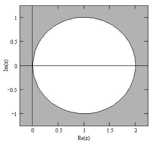
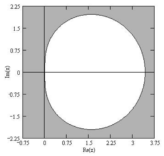
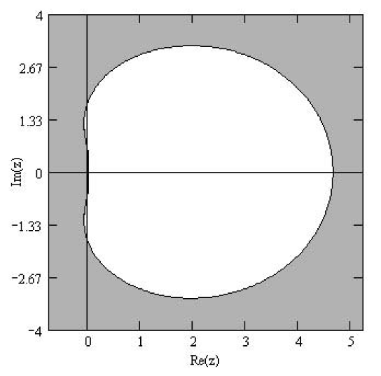
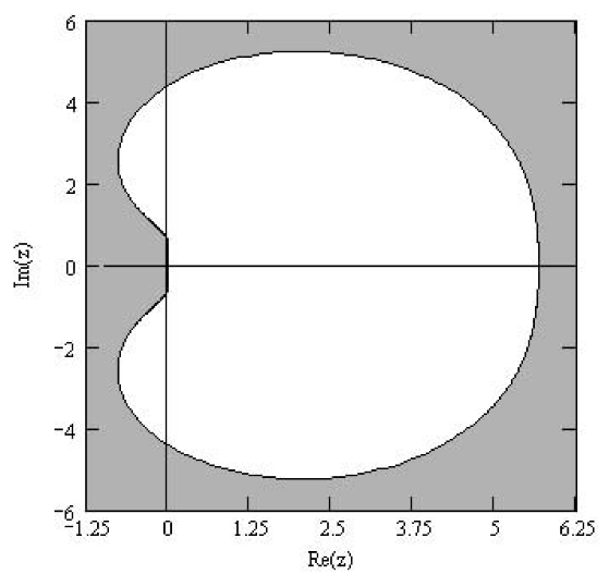
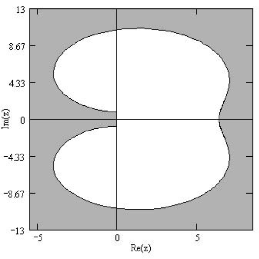
Figure 1: stability regions for $(m+1)$th LIL method: a) $m=1$; b) $m=2$; c) $m=3;$ d) $m=4$; e) $m=5$.

Taking account of the fact that higher order is not always higher accuracy, an acceptable compromise between the accuracy, time stability and computational time was proved to be  $m=3$.

5 Applications

5.1 LIL versus standard methods

The goal of this section is to compare the characteristics of few known standard algorithms (the 4th-order   methods: Runge-Kutta, Gear, Adams-Moulton, the 3th-order Adams-Bashforth method and the Milne method) and 4th-order LIL method. For this purpose we integrated two simple examples, with known analytical solutions: the Bernoulli equation

$$2\,t^{2}\overset{.}{x}(t)-4\,t\,x(t)-x^{2}(t)=0,\,$$

and

$$\overset{.}{x\,}(t)=\cos(t).\,$$

The following values were calculated:

- the relative error  $\varepsilon_{r}=\sum\left|x_{a}-x\right|/\sum x_{a}\,,\ \$where $x_{a}\,$ is the analytical solution. The sum is taken over the integration interval.

- the maximum absolute error: $\Delta=\underset{k}{\max}\left|x_{a,k}-x_{k}\right|,\,$ where $x_{a,k}$  is the exact solution in  $t_{k}.$

- the computation time $t$

The results are presented in Table 5 and 6.

(a)	R-K	Gear	A-M	A-B	Milne	LIL
$\varepsilon_{r}$	1.9$\cdot 10^{-4}$	1.9$\cdot 10^{-4}$	1.1$\cdot 10^{-7}$	1.1$\cdot 10^{-7}$	1.4$\cdot 10^{-7}$	1.4$\cdot 10^{-7}$
$\Delta$	1.9$\cdot 10^{-2}$	2.0$\cdot 10^{-2}$	1.2$\cdot 10^{-5}$	1.2$\cdot 10^{-5}$	1.8$\cdot 10^{-5}$	1.5$\cdot 10^{-5}$
t[s]	0.16	0.16	0.16	0.10	0.10	0.16

(b)	R-K	Gear	A-M	A-B	Milne	LIL
$\varepsilon_{r}$	3.8$\cdot 10^{-5}$	3.8$\cdot 10^{-5}$	2.3$\cdot 10^{-10}$	2.3$\cdot 10^{-10}$	2.8$\cdot 10^{-10}$	2.8$\cdot 10^{-10}$
$\Delta$	1.9$\cdot 10^{-3}$	2.0$\cdot 10^{-3}$	1.2$\cdot 10^{-8}$	1.8$\cdot 10^{-8}$	1.8$\cdot 10^{-8}$	1.5$\cdot 10^{-8}$
t[s]	0.82	0.71	0.82	0.43	0.71	0.87

Table 5: Bernoulli equation integrated with: a) $h=0.01,~{}$ $t\in[1,100]$; b) $h=0.001$,  $t\in[1,50].$

$(a)$	R-K	Gear	A-M	A-B	Milne	LIL
$\varepsilon_{r}$	2.4$\cdot 10^{-2}$	4.9$\cdot 10^{-2}$	7.7$\cdot 10^{-4}$	4.0$\cdot 10^{-3}$	5.0$\cdot 10^{-3}$	5.0$\cdot 10^{-3}$
$\Delta$	3.7$\cdot 10^{-2}$	5.3$\cdot 10^{-2}$	4.9$\cdot 10^{-4}$	2.6$\cdot 10^{-3}$	3.9$\cdot 10^{-3}$	3.3$\cdot 10^{-3}$
t[s]	$0.0$	0.0	0.0	0.0	0.0	0.0

$(b)$	R-K	Gear	A-M	A-B	Milne	LIL
$\varepsilon_{r}$	$4.9\cdot 10^{-4}$	$9.9\cdot 10^{-4}$	$3.9\cdot 10^{-7}$	1.5$\cdot 10^{-6}$	1.9$\cdot 10^{-6}$	$1.9\cdot 10^{-6}$
$\Delta$	$7.5\cdot 10^{-4}$	$1.0\cdot 10^{-3}$	$2.4\cdot 10^{-7}$	2.7$\cdot 10^{-7}$	1.5$\cdot 10^{-6}$	$1.2\cdot 10^{-6}$
t[s]	$0.16$	0.16	0.16	0.16	0.16	0.16

Table 6: $\dot{x}(t)=\cos(t)$, $t\in[0,2\pi]$ integrated with: a) $h=0.05$; b) $h=0.001$.

Comparing the results in Tables 5 and 6 one can deduce that LIL’s performances, for these two examples, are comparable to those of performant methods like Gear, Adams-Moulton and Adams-Bashforth.

5.2 Rabinovich-Fabrikant system

The hard test was the integration of the Rabinovich-Fabrikant system. Rabinovich and Fabrikant [6] studied the following dynamical system (named the R-F model hereafter)

$$\begin{array}[]{l}\overset{.}{x_{1}}=x_{2}(x_{3}-1+x_{1}^{2})+ax_{1},\\[3.0pt] \overset{.}{x_{2}}=x_{1}(3x_{3}+1-x_{1}^{2})+ax_{2},\\[3.0pt] \overset{.}{x_{3}}=-2x_{3}(b+x_{1}x_{2}),\end{array}\quad\qquad a,b\in\mathbb{R}.$$ (18)

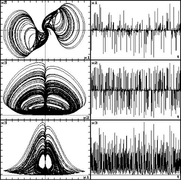
Figure 2: Two chaotic trajectories of R-F system: a) Three-dimensional phase portrait for $a=0.1$,  $b=0.2876$; b) Plane phase portraits and time series for $a=-1$,   $b=-0.1$.

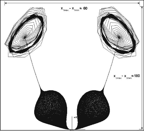
Figure 3: Two different sizes of the same attractor obtained with different step-sizes: a) for  $h=5\times 10^{-3},$  $x_{3\max}=35$  while b) for  $h=5\times 10^{-4},$  $x_{3\max}=350.$

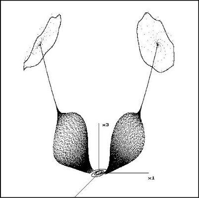
Figure 4: Two different attractors (plotted here by points), with the same initial conditions and parameters values ($a=0.12,$  $b=0.05)$, but with different step-size  a) $h=0.05$  and  b) $h=0.005.$

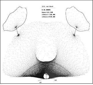
Figure 5: The case  $a=0.3$  and  $b=0.1$  integrated with: a) the 4th-order Adams-Moulton ; b) the 4th-order Gear algorithm; c) 3th Adams-Bashforth algorithm; d) 4th-LIL algorithm.

This system models the stochasticity arising from the modulation instability in a non-equilibrium dissipative medium. Some qualitative analysis and numerical dynamics have been reported in [6] and a carefully re-examination together with many new and rich complex dynamics of the model, that were mostly not reported before, are presented in [3]. The chaotic R-F model proved to be a great challenge to the classical numerical methods, most of them being not successful to study the complex dynamics of this special model.

All computer test results and graphical plots in Figures 2-5 were obtained with a special Turbo Pascal code which plots phase diagrams and time series  The code for LIL method may be obtained directly from the author.

For $a<b$, the system is characterized by the appearance of chaotic attractors in the phase space (see e.g. Figures 2).

It is well known that because of the sensitive dependence on initial data, a chaotic system tends to amplify, often exponentially, tiny initial errors. These kind of errors could be amplified to so large, that it is almost impossible to draw mathematically rigorous conclusions based on numerical simulations. A typical case can be seen from Figure 3, wherefrom one deduces that the attractor’s size along the $x_{3}$-axis increases significantly as the step-size decreases. This problem has been noticed for a long time, and has promoted a useful theory called “shadowing,” namely, the existence of a true orbit nearby a numerically computed approximate orbit [1]. We have also found that the strong dependence on the step-size for R-F system, for certain values of $\ b$ and with the same initial conditions, could produce totally different attractors (see Figures 4)

There are few special cases which proved to be a real challenge for the numerical methods. As example for the case $\ a=0.3$  and  $b=0.1$ (shown in Figure 3), the 4th-order Runge-Kutta and Milne methods failed while only the Gear and Adams-Moulton methods seem to give comparable results to those obtained with LIL method; the attractors obtained with the 3th-order Adams-Bashforth method are different to those obtained with Gear, Adams-Moulton and LIL methods (Figures 5).

6 Concluding remarks

In this paper we present a linear implicit multi-step method, LIL, for ODEs proving its convergence, too. The method could be considered as an acceptable alternative to the classical algorithms for ODEs and can be successfully used in practical applications. One of the advantages is that in (5) only the even order derivatives appear, this fact reducing the truncation error and the computational time.

The algorithm seems to be stiffly-stable since it can integrate efficiently and accurately enough dynamical systems like R-F which presents stiff characteristics.

The implementation of adaptive step-size represents a task for a future work. The basic approach would be applicable directly to variable step-size.

7 Acknowledgments

The author acknowledges Professor T. Coloşi, the promoter of this method, for his continuous encouragement and discussions on this work.

Appendix
$i=2$ $\delta_{20}$ $\delta_{21}$ $\delta_{22}$ $\delta_{23}$ $\delta_{24}$ $\delta_{25}$ $m=2$ 1 -2 1 $\cdots$ $\cdots$ $\cdots$ $m=3$ 2 -5 4 -1 $\cdots$ $\cdots$ $m=4$ 35/12 -26/3 19/2 -14/3 11/12 $\cdots$ $m=5$ 15/4 -77/6 107/6 -13 61/12 -5/6 $i=3$ $\delta_{30}$ $\delta_{31}$ $\delta_{32}$ $\delta_{33}$ $\delta_{34}$ $\delta_{35}$ $m=3$ 1 -3 3 -1 $\cdots$ $\cdots$ $m=4$ 5/2 -9 12 -7 3/2 $\cdots$ $m=5$ 17/4 -71/4 59/2 -49/2 41/4 -7/4 $i=4$ $\delta_{40}$ $\delta_{41}$ $\delta_{42}$ $\delta_{43}$ $\delta_{44}$ $\delta_{45}$ $m=4$ 1 -4 6 -4 1 $\cdots$ $m=5$ 3 -14 26 -24 11 -2

$i=5$	$\delta_{50}$	$\delta_{51}$	$\delta_{52}$	$\delta_{53}$	$\delta_{54}$	$\delta_{55}$
$m=5$	1	-5	10	-10	5	-1

Table 7: $\delta$ coefficients.

$(a)$	$m=1$	$m=$2	$m=$3	$m=$ 4	$m=5$
$\sigma_{00}$	1	25/24	13/12	6463/5760	741/640
$\sigma_{01}$	0	-1/12	-5/24	-523/1440	-1561/2880
$\sigma_{02}$	$\cdots$	1/24	1/6	383/960	2179/2880
$\sigma_{03}$	$\cdots$	$\cdots$	-1/24	-283/1440	-133/240
$\sigma_{04}$	$\cdots$	$\cdots$	$\cdots$	223/5760	1253/5760
$\sigma_{05}$	$\cdots$	$\cdots$	$\cdots$	$\cdots$	-103/2880

$(b)$	$m=1$	$m=$2	$m=$3	$m=$4	$m=$5
$\sigma_{10}$	1	3/2	15/8	35/16	315/128
$\sigma_{11}$	-1	-2	-25/8	-35/8	-735/128
$\sigma_{12}$	$\cdots$	1/2	13/8	7/2	399/64
$\sigma_{13}$	$\cdots$	$\cdots$	-3/8	-13/8	-279/64
$\sigma_{14}$	$\cdots$	$\cdots$	$\cdots$	5/16	215/128
$\sigma_{15}$	$\cdots$	$\cdots$	$\cdots$	$\cdots$	-35/128

Table 8: $\sigma$ coefficients.

$m$	$\varepsilon_{m1}$	$\varepsilon_{m2}$	$\varepsilon_{m3}$	$\varepsilon_{m4}$	$\varepsilon_{m5}$
$2$	2	-1	$\cdots$	$\cdots$	$\cdots$
$3$	3	-3	1	$\cdots$	$\cdots$
$4$	4	-6	4	-1	$\cdots$
$5$	5	-10	10	-5	1

Table 9: $\varepsilon$ coefficients.