High-Spatial-Resolution Monitoring of Strong Magnetic Field using Rb vapor Nanometric-Thin Cell

Abstract

We have implemented the so-called $\lambda$-Zeeman technique (LZT) to investigate individual hyperfine transitions between Zeeman sublevels of the Rb atoms in a strong external magnetic field $B$ in the range of $2500-5000$ G (recently it was established that LZT is very convenient for the range of $10-2500$ G). Atoms are confined in a nanometric thin cell (NTC) with the thickness $L=\lambda$, where $\lambda$ is the resonant wavelength 794 nm for Rb $D_{1}$ line. Narrow velocity selective optical pumping (VSOP) resonances in the transmission spectrum of the NTC are split into several components in a magnetic field with the frequency positions and transition probabilities depending on the $B$-field. Possible applications are described, such as magnetometers with nanometric local spatial resolution and tunable atomic frequency references.

1 Introduction

A number of optical and magneto-optical processes running at interaction of a narrow-band laser radiation with atomic vapors are employed in laser technology, metrology, designing of high-sensitivity magnetometers, problems of quantum communications, information storage etc [1, 2]. As known, the energy levels of atoms undergo frequency shifts and changes in their transition probabilities in an external magnetic field $B$. The related effects were studied for hyperfine (hf) atomic transitions in optical domain for the transmission spectra obtained with an ordinary cm-size cell containing Rb and Cs vapor in [3]. However, because of Doppler broadening (hundreds of MHz), it was possible to partially separate different hf transitions only for $B>1500$ G. Note that even for these large $B$ values the lines of the ⁸⁵Rb and the ⁸⁷Rb are strongly overlapped, and pure isotopes should be used to avoid complicated spectra. In order to eliminate the Doppler broadening, the well-known saturation absorption (SA) technique was implemented to study the Rb hf transitions [4, 5]. However, in this case the complexity of the Zeeman spectra in a magnetic field arises primarily from the presence of strong crossover resonances, which are also split into many components. That is why, the SA technique is applicable only for $B<100$ G. Another significant disadvantage is the fact that the SA is strongly nonlinear and, therefore, the peak amplitudes of the decreased absorption do not correspond to probabilities of atomic transitions at frequencies of which these peaks are formed. This additionally complicates the processing of the spectra. The crossover resonances can be eliminated with selective reflection spectroscopy [6], but to correctly determine the hf transition position, the spectra must undergo further non-trivial processing. It was demonstrated in [7, 8] that the use of resonance fluorescence spectra of a NTC filled with Rb atomic vapor and having a thickness of $L=0.5\lambda$ (where $\lambda=794$ nm is the wavelength of laser radiation whose frequency is resonant to the atomic transition of the $D_{1}$ line of Rb) allows one to separate and to study the atomic transitions between the levels of the hyperfine structure of the $D_{1}$ line of the ⁸⁷Rb atoms in magnetic fields with $B=10-200$ G. The achieved high sub-Doppler spectral resolution is caused by the effect of a strong narrowing of the fluorescence spectrum of a NTC with the atomic vapor column thickness $L=\lambda/2$. With the proper choice of the laser intensity and NTC temperature, it is possible to achieve an eightfold narrowing of the spectrum compared to that in ordinary $1-10$ cm-long cells (for which the Doppler width is about 500 MHz). The method was called ”half-lambda Zeeman technique” (HLZT). In [9, 10], the $D_{2}$ lines of Rb and Cs atoms were studied using HLZT in magnetic fields of about 50 G. Recently it has been shown that the use of the HLZT allows one to perform detailed quantitative measurements of both frequency characteristics and probabilities of large number of atomic transitions between levels of the hyperfine structure of the Rb $D_{1}$ line in magnetic fields ranging within 10 – 2500 G [11]. In [12, 13] it is described a technique based on the use of spectrally-narrow (close to natural line-width) velocity selective optical pumping (VSOP) resonances peaks appearing at laser intensities $\sim 10$ mW/cm² exactly at the positions of atomic transitions in the transmission spectrum of the NTC with the Rb vapor column thickness of $L=\lambda$ ($\lambda$ being the wavelength of laser radiation resonant with Rb $D_{1}$ or $D_{2}$ atomic lines, 794 or 780 nm). Each VSOP resonance is split in an external magnetic field into several Zeeman components, the number of which depends on the quantum numbers $F$ of the lower and upper levels. The amplitudes of these components and their frequency positions depend unambiguously on $B$-field. Hence, with the use of LZT it is also possible to study not only the frequency shift of any individual hf Zeeman transition, but also the modification in transition probability. The efficiency of LZT has been proved in the region of 1 - 2500 G [13]. Among the most interesting results obtained through HLZT and LZT implementation are vanishing of some of atomic transitions for specific $B$-field strength, and the appearance of $\Delta F=2$ transitions, which are forbidden for $B=0$ [13]. Moreover, the line intensity of a forbidden transition for some value of magnetic field can be higher than that for strong atomic transitions when $B=0$. It is important to note that LZT could have several advantages as compared with the HLZT: in particular, the spectral width of VSOP resonances used in LZT is at least 4 times narrower than that used in HLZT, resulting in much higher resolution; also the laser power required for LZT is $\sim 10$ times lower than that needed for HLZT; and finally, recording of resonant transmission spectra does not require sensitive detectors as in the case of fluorescence spectra. The aim of the work is to demonstrate that LZT can also be successfully used for even higher external magnetic fields up to 5000 G. Possible applications of LZT for diagnostics and mapping of large magnetic gradients and for making widely tunable compact frequency references are addressed too.

2 Experiment

2.1 Nanometric-thin cell

The first design of the NTC (called extremely thin cell) consisting of windows and a vertical side-arm (a metal reservoir), was presented in [14]. Later, this design was somewhat modified and a typical example of recent version is presented in [15]. The photograph of the NTC with smoothly variable thickness wedged in the vertical direction is shown in Fig. 2. The wedged gap in this case was formed using a platinum spacer strip of 2 $\mu$m thickness. The presented NTC has garnet windows of 0.8 mm thickness (the use of thin wafers in some cases is more convenient), and in order to increase the wafers thickness at the bottom to fit the side-arm ($\varnothing=$ 2 mm), two additional garnets plates are glued to the main wafers. The NTC is filled with a natural mixture of the ⁸⁵Rb ($72.2\%$) and ⁸⁷Rb ($27.8\%$). The region of $L\approx\lambda\approx 800$ nm is indicated. The temperature limit of the NTC operation is 400 ^∘C. The NTC operated with a specially designed oven with two ports for laser beam transmission. The source temperature of the atoms of the NTC was 120 ^∘C, corresponding to the vapor density $N=2\cdot 10^{13}$cm^-3, but the windows were maintained at a temperature that was 20 ^∘C higher.

2.2 Experimental setup

The sketch of the experimental setup is shown in Fig. 2. The circularly polarized beam of extended cavity diode laser (ECDL, $\lambda=794$ nm, $P_{L}=30$ mW, $\gamma_{L}<1$ MHz) resonant with the ⁸⁷Rb $D_{1}$ transition frequency, was directed onto the Rb NTC (2) with the vapor column thickness $L=\lambda=794$ nm at nearly normal incidence. The NTC was inserted in a special oven with two openings. The transmission signal was detected by a photodiode (4) and was recorded by Tektronix TDS 2014B digital four-channel storage oscilloscope (5). A Glan prism was used to purify initial linear radiation polarization of the laser radiation; to produce a circular polarization, a $\lambda/4$ plate (1) was utilized. Magnetic field was directed along the laser radiation propagation direction k ($\textbf{B}\|\textbf{k}$). About $50\%$ of the pump power was branched by a beam splitter to an auxiliary Rb NTC ($2^{\prime}$).

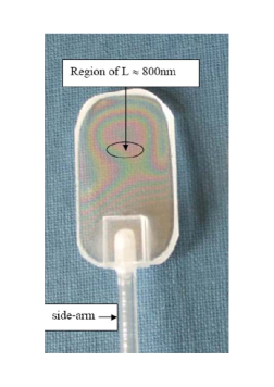
Figure 1: Photography of the NTC. Since NTC gap thickness is of order of visible light wavelength, interferometric pattern occurs. Region of $L=\lambda=800$ nm is indicated, NTC has a sapphire side-arm.

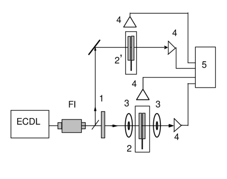
Figure 2: Sketch of the experimental setup. ECDL - diode laser, FI - Faraday isolator, $1$ - $\lambda/4$ plate, $2$ - NTC in the oven, $2^{\prime}$ - an auxiliary NTC and the oven, $3$ - ring magnets, $4$ - photodetectors, $5$ - digital storage oscilloscope.

The fluorescence spectrum of the latter at $L=\lambda/2$ was used as a frequency reference for $B=0$. Moderate longitudinal magnetic field ($B<250$ G) was applied to the NTC by a system of Helmholtz coils (not shown in Fig. 2). The $B$-field strength was measured by a calibrated Hall gauge. It is important to note that the use of the NTC allows one to apply very strong magnetic fields using widely available strong permanent ring magnets (PRM): in spite of strong inhomogeneity of magnetic field (in our case it can reach 150 G/mm), the variation of $B$-field inside atomic vapor column is $\sim 0.1$ G, i.e. by several orders less than the applied $B$ value, thanks to small thickness of the NTC ($L=794$ nm).

2.3 Experimental results and discussion

The allowed transitions between magnetic sublevels of hf states for the ⁸⁵Rb and ⁸⁷Rb, $D_{1}$ line in the case of $\sigma^{+}$ (left circular) polarized excitation and selection rules $\Delta m_{F}=+1$ are depicted in Fig. 3 (LZM works well also for $\sigma^{-}$ excitation). In [13] the maximum attainable strength of $B$-field was 2500 G. In order to increase the attainable strength of the external magnetic field applied to the atomic vapor contained in NTC, the permanent ring magnets embracing the cell should be as close to each other as possible. The main limitation for the distance between PRMs is imposed by the longitudinal dimension of the cell oven (see Fig. 2). Earlier, in [13] the longitudinal dimension of the oven was 4 cm resulting in the maximum attainable strength of 2500 G. A new oven was developed specially for high $B$-field applications, with the longitudinal dimension of $\approx 2$ cm. This allows us to produce the attainable strength of $B$-field $>2500$ G.

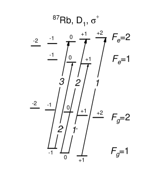
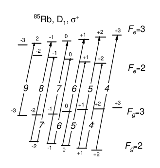
Figure 3: The hfs energy level diagram of $D_{1}$ line of ⁸⁷Rb (a) and ⁸⁵Rb (b) in magnetic field and possible atomic Zeeman transitions for $\sigma^{+}$ polarized exciting laser radiation.

As it was shown [13] LZT is based on the use of spectrally-narrow VSOP resonances appearing at laser intensities $\sim 10$ mW/cm² in the transmission spectrum of the NTC with the thickness $L=\lambda$. The VSOP peaks of reduced absorption are exactly at the atomic transitions, and these VSOPs are split into several new components, the number of which depends on the quantum numbers $F$ of the lower and upper levels, while the amplitudes of the components and their frequency positions depend on $B$-field. Fig. 4 shows the NTC transmission spectra for $L=\lambda$ for the allowed transitions between magnetic sublevels of hf states for the ⁸⁵Rb and ⁸⁷Rb, $D_{1}$ line in the case of $\sigma^{+}$ polarized excitation at $B=2910$ G (the upper curve) and $B=2430$ G (the middle curve). The labels $1-8$ denote the corresponding transitions between the magnetic sublevels shown in Fig. 3. As shown, all the individual Zeeman transitions are clearly detected. The lower grey curve presents the fluorescence spectrum of the NTC of $L=\lambda/2$, which is the reference spectrum for the case $B=0$. For convenience the spectra are shifted vertically.

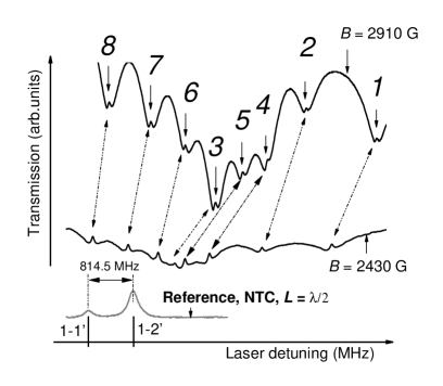
Figure 4: NTC transmission spectra for $L=\lambda$ for the transition between sublevels of hf states for the ⁸⁵Rb and ⁸⁷Rb $D_{1}$ line in the case of $\sigma^{+}$ excitation at $B=2910$ G (the upper curve) and $B=2430$ G (middle curve). The lower grey curve presents the reference spectrum, which is the fluorescence spectrum of the NTC of $L=\lambda/2$, for $B=0$. Oblique arrows indicate the positions of the VSOPs resonance frequencies with the labels $1-8$ for $B=2430$ G and $B=2910$ G.

The oblique arrows indicate the positions of the VSOP resonances with the labels $1-8$ for $B=2430$ and 2910 G. As seen from Fig. 4 for magnetic field measurement the most convenient is the VSOP peak number 1 (⁸⁷Rb, $F_{g}=1$, $m_{F}=+1\rightarrow F_{e}=2$, $m_{F}=+2$), since it has the largest peak amplitude among transitions 1, 2, 3 of the ⁸⁷Rb and it is not overlapped with any other transition, while having a strong detuning value of $\sim 1.8$ MHz/G versus magnetic field strength. It is important to note that LZT allows one to check whether the VSOP resonance (i.e. peak of reduced absorption) is a real one or has an artificial/noise nature. For this purpose one should simply increase the side-arm temperature by additional 20 – 30 degrees in order to provide larger absorption in the transmission spectrum. The real VSOP must be located exactly at the bottom of the absorption at the position of the corresponding atomic transition shifted in the magnetic field, as it is shown on the upper curve of Fig. 4 (the side-arm temperature is 140 ^∘C). As it is mentioned the strong magnetic field is produced by two PRMs ($\varnothing=$ 30 mm), with holes ($\varnothing=$ 3 mm) to allow radiation to pass, placed on opposite sides of the nanocell oven and separated by a distance varied between 20 mm and 35 mm (see Fig. 2). To control the magnetic field value, one of the magnets was mounted on a micrometric translation stage for longitudinal displacement.

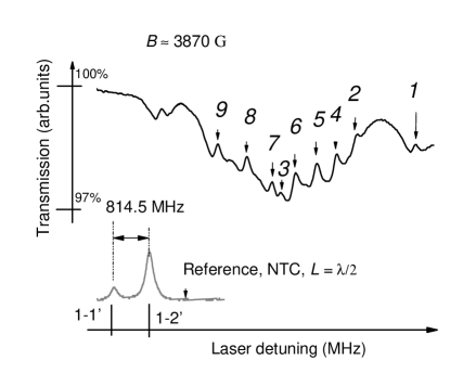
Figure 5: NTC transmission spectra for $L=\lambda$ for the transition between sublevels of hf states for the ⁸⁵Rb and ⁸⁷Rb $D_{1}$ line for the case of $\sigma^{+}$ excitation at 3870 G (the upper curve). The lower grey curve presents the reference spectrum, which is the fluorescence spectrum of the NTC of $L=\lambda/2$, for $B=0$.

The NTC transmission spectra for the thickness $L=\lambda$, for the ⁸⁵Rb and ⁸⁷Rb, $D_{1}$ line in the case of $\sigma^{+}$ excitation at $B=3870$ G (the upper curve) are presented in Fig. 5. The labels $1-9$ denote the corresponding transitions between the magnetic sublevels shown in Fig. 3. The lower grey curve presents the fluorescence spectrum of the NTC of $L=\lambda/2$, which is the reference spectrum for the case $B=0$. A new VSOP with label 9 is seen in the spectrum (the corresponding atomic transition is shown in Fig. 3), while it was absent for the case of smaller $B$-field shown in Fig. 4. As it is seen from Fig. 5 the most convenient is still the VSOP peak number 1 for magnetic field measurement. The following control experiment was carried out: one of PRMs was set on the table with the micrometer step. In the magnetic field $\sim 4000$ G, one PRM was shifted toward the other by the displacement of PRMs by 15 $\mu$m leading to the frequency shift of component 1 by 4 MHz to the high frequency region, which was detected by the comparison of the spectra relatively easy.

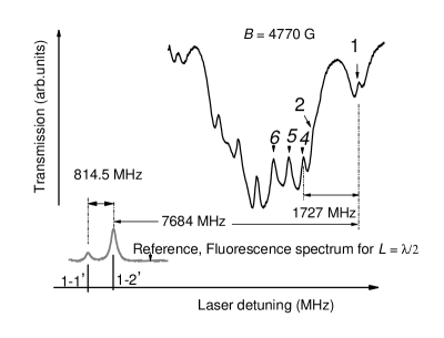
Figure 6: NTC transmission spectra for $L=\lambda$ for the ⁸⁵Rb and ⁸⁷Rb $D_{1}$ line in the case of $\sigma^{+}$ excitation at $B=4770$ G (the upper curve). The lower grey curve presents the reference spectrum, which is the fluorescence spectrum of the NTC of $L=\lambda/2$, for $B=0$.

The NTC transmission spectra for thickness $L=\lambda$, for the ⁸⁵Rb and ⁸⁷Rb, $D_{1}$ line in the case of $\sigma^{+}$ excitation at $B=4770$ G (the upper curve) is presented in Fig. 6. The labels $1-6$ denote the corresponding transitions between the magnetic sublevels shown in Fig. 3. The lower grey curve presents the fluorescence spectrum of the NTC of $L=\lambda/2$, which is the reference spectrum for the case $B=0$. As it is seen from Fig. 6 the VSOP peak number 1 is still the most convenient for magnetic field measurement. We note that transition 1 is strongly shifted by $\sim 7.7$ GHz from the $B=0$ position of the $F_{g}=1\rightarrow F_{e}=2$ transition. The latter allows allows of developing a frequency reference based on a nanocell and PRMs, widely tunable over a range of several gigahertz onto high-frequency wing of transition of ⁸⁷Rb atom by simple displacement of the magnet.

3 Theoretical model and discussions

In this work the main interest is to study the behavior of the ⁸⁷Rb, $F_{g}=1\rightarrow F_{e}=2$ transitions, $D_{1}$ line in the case of $\sigma^{+}$ excitation, since from the application point of view they are most interesting. Note, that for $\sigma^{-}$ excitation the probability of the atomic transitions rapidly decreases with magnetic field strength. Also, the probability of the atomic transitions ⁸⁷Rb, $F_{g}=1\rightarrow F_{e}=1$ in the case of $\sigma^{+}$ excitation rapidly decreases with magnetic field strength. Theoretical model describes how to provide the calculations of separated transition’s frequencies and amplitude modification undergo external magnetic field [3, 6, 7, 8, 9, 10, 16]. We adopt a matrix representation in the coupled basis, that is, the basis of the unperturbated atomic state vectors $\left|(n=3),L,J,F,m_{F}\right\rangle$ to evaluate the matrix elements of the Hamiltonian describing our system. In this basis, the diagonal matrix elements are given by

$$\left\langle F,m_{F}|H|F,m_{F}\right\rangle=E_{0}(F)+\mu_{B}g_{F}m_{F}B_{Z},$$ (1)

where $E_{0}(F)$ is the initial energy of the sublevel $\left|(n=3),L,J,F,m_{F}\right\rangle\equiv\left|F,m_{F}\right\rangle$ and $g_{F}$ is the effective Landé factor. The off-diagonal matrix elements are non-zero for levels verifying the selection rules $\Delta L=0,\Delta J=0,\Delta F=\pm 1,\Delta m_{F}=0$,

$$\begin{array}[]{r}\left\langle F-1,m_{F}|H|F,m_{F}\right\rangle=\left\langle F,m_{F}|H|F-1,m_{F}\right\rangle=-\frac{\mu_{B}B_{z}}{2}(g_{J}-g_{I})\\ \times\left(\frac{[(J+I+1)^{2}-F^{2}][F^{2}-(J-I)^{2}]}{F}\right)^{1/2}\left(\frac{F^{2}-m_{F}^{2}}{F(2F+1)(2F-1)}\right)^{1/2}.\end{array}$$ (2)

The diagonalization of the Hamiltonian matrix allows one to find the eigenvectors and the eigenvalues, that is to determine the eigenvalues corresponding to the energies of Zeeman sublevels and the new states vectors which can be expressed in terms of the initial unperturbed atomic state vectors,

$$\left|\Psi(F_{e}^{{}^{\prime}},m_{F_{e}})\right\rangle=\sum_{F_{e}=I-J_{e}}^{F_{e}=I+J_{e}}\alpha_{F_{e}^{{}^{\prime}}F_{e}}^{e}(B_{z},m_{F_{e}})|F_{e},m_{F_{e}}\rangle$$ (3)

and

$$\left|\Psi(F_{g}^{{}^{\prime}},m_{F_{g}})\right\rangle=\sum_{F_{g}=I-J_{g}}^{F_{g}=I+J_{g}}\alpha_{F_{g}^{{}^{\prime}}F_{g}}^{g}(B_{z},m_{F_{g}})|F_{g},m_{F_{g}}\rangle.$$ (4)

The state vectors $\left|F_{e},m_{e}\right\rangle$ and $\left|F_{g},m_{g}\right\rangle$ are the unperturbated state vectors, respectively, for the excited and the ground states. The coefficients $\alpha_{F_{e}^{{}^{\prime}}F_{e}}^{e}(B_{z},m_{F_{e}})$ and $\alpha_{F_{g}^{{}^{\prime}}F_{g}}^{g}(B_{z},m_{F_{g}})$ are mixing coefficients, respectively, for the excited and the ground states; they depend on the field strength and magnetic quantum numbers $m_{e}$ or $m_{g}$. Diagonalization of the Hamiltonian matrix for ⁸⁷Rb, $D_{1}$ line, in case of $\sigma^{+}$ polarization of exciting radiation, allows one to obtain the shift of position of energy levels in presence of external magnetic field.

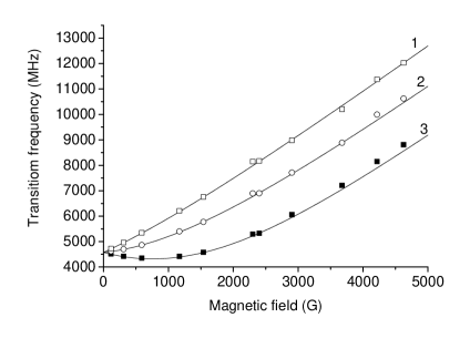
Figure 7: Transition’s frequency of components $1$, $2$ and $3$ relatively to the initial position at $B=0$, solid line is the theory.

Fig. 7 shows the frequency shift of components 1, 2 and 3 (see diagram in Fig. 3) relative to their initial position at $B=0$. The probability of a transition, induced by the interaction of the atomic electric dipole and the oscillating laser electric field is proportional to the spontaneous emission rate of the associated transition $A_{eg}$, that is, to the square of the transfer coefficients modified by the presence of the magnetic field

$$\frac{8\pi^{2}}{3\varepsilon_{0}\hbar\lambda_{eg}^{3}}\left|\left\langle e\left|D_{q}\right|g\right\rangle\right|^{2}=A_{eg}\propto a^{2}\left[\Psi(F_{e}^{{}^{\prime}},m_{F_{e}});\Psi(F_{g}^{{}^{\prime}},m_{F_{g}});q\right],$$ (5)

where $D_{q}$ denote the standard components of the electric dipole moment:

$$\vec{D}.\vec{e}=\sum_{q}D_{q}e_{q},$$ (6)

with $q=-1,0,1$. In Eq. (5), the transfer coefficients are expressed as

$$a\left[\Psi(F_{e}^{{}^{\prime}},m_{F_{e}});\Psi(F_{g}^{{}^{\prime}},m_{F_{g}});q\right]=\sum_{F_{e}F_{g}}\alpha_{F_{e}^{{}^{\prime}}F_{e}}^{e}(B_{z},m_{F_{e}})a\left(F_{e},m_{F_{e}};F_{g},m_{F_{g}};q\right)\alpha_{F_{g}^{{}^{\prime}}F_{g}}^{g}(B_{z},m_{F_{g}}),$$ (7)

where the unperturbated transfer coefficients have the following definition

$$\begin{array}[]{l}{a\left(F_{e},m_{F_{e}};F_{g},m_{F_{g}};q\right)=(-1)^{1+I+J_{e}+F_{e}+F_{g}-m_{F_{e}}}}\\ {\times\sqrt{2J_{e}+1}\sqrt{2F_{e}+1}\sqrt{2F_{g}+1}\left(\begin{array}[]{ccc}F_{e}&1&F_{g}\\ -m_{F_{e}}&q&m_{F_{g}}\end{array}\right)\left\{\begin{array}[]{ccc}F_{e}&1&F_{g}\\ J_{g}&I&J_{e}\end{array}\right\}}\end{array},$$ (8)

the parenthesis and curly brackets denote, respectively, the $3j$ and $6j$ symbols, $g$ and $e$ point respectively ground and excited states.

Figure 8: (a) The probability for the atomic transition $1,2,3$ in the case of $\sigma^{+}$ excitation versus magnetic field (theory), (b) curve 1 shows the ratio of the amplitudes $A(1)/A(3)$ and curve 2 shows the ratio of the amplitudes $A(1)/A(2)$ versus $B$.

Fig. 8 shows the probability for the atomic transitions 1, 2, 3 (i.e. the atomic line intensity) for the case of $\sigma^{+}$ excitation versus magnetic field for (theory) versus $B$. However, in the experiment it is more convenient to measure the ratio of the VSOPs amplitudes $A1$, $A2$ and $A3$ of transitions 1, 2 and 3 versus $B$ (shown in Fig. 8), since the absolute value of the VSOP amplitude depends on laser intensity, NTC temperature, etc. Note that for $B\approx 0$ the ratios $A1:A2:A3=6:3:1$ , while for large $B$, these ratios become $A1\approx A2\approx A3$. Also, as it is seen for $B$ up to 5000 G the VSOP amplitude $A1$ is increasing, which makes it convenient to use VSOP with label 1 for a magnetic field measurement. It is obvious that a NTC with an oven can also be fixed on a table with a micrometer step so that the displacements of this system allow one to map strongly inhomogeneous magnetic fields. For a more successful mapping, the dimensions of the NTC with oven could, in principle, be decreased further; i.e., a conducting and optically transparent deposited layer can replace the oven and the window thickness can be reduced to 100 $\mu$m with the reduction of the transverse dimensions of the NTC down a few millimeters. It should be noted that, with regard to sensitivity, the magnetometer based on LZT is far below magnetometers based on coherent processes [1, 2], but has advantages in the measurement of strong and gradient magnetic fields. Note also that the spectral resolution achieved by LZT may also be realized with the use of well-collimated atomic beams (by means of 3 - 4 m vacuum pipes where the beam will be formed) or plants for cooling of atoms. However, employment of the atomic-beam technology or atom cooling is very complicated and expensive problem, whereas LZT requires only available cheap diode lasers and a nanocell filled with alkali metal.

4 Conclusion

The ”$\lambda$-Zeeman technique” is shown to be a convenient and robust tool for the study of individual transitions between the Zeeman sublevels of hyperfine levels in an external magnetic field of 10 - 5000 G (taking into account previously obtained results of the LZT use for the range of 10 - 2500 G). LZT is based on NTC resonant transmission spectrum with thickness $L=\lambda$, where $\lambda$ is the resonant wavelength (794 nm) for $D_{1}$ line of the Rb. Narrow VSOP resonances (of $\sim 20-30$ MHz linewidth) in the transmission spectrum of the NTC are split into several components in a magnetic field; their frequency positions and transition probabilities depend on the $B$ field. Examination of the VSOP resonances formed in a nanometric-thin cell allows one to obtain, identify, and investigate the atomic transitions between the Zeeman sublevels in the transmission spectrum of the ⁸⁷Rb $D_{1}$ line in the range of magnetic fields 10 - 5000 G. Nanometric-thin column thicknesses ($\sim$ 794 nm) allow of the application of permanent magnets, which facilitates significantly the creation of strong magnetic fields. The results obtained show that a nano - magnetometer in the range of 10 - 5000 G with a local spatial resolution of $\sim$ 794 nm can be created based on a NTC and the atomic transition of the ⁸⁷Rb $D_{1}$, $F_{g}=1,m_{F}=+1\rightarrow F_{e}=2,m_{F}=+2$. This result is important for mapping strongly inhomogeneous magnetic fields. LZT can be successfully implemented also for the case of Cs, Na, K, Li atoms. Experimental results are in a good agreement with the theoretical values.

5 Acknowledgements

The authors are grateful to A. Sarkisyan for his valuable participation in fabrication of the NTC as well as to A. Papoyan and A. Sargsyan for useful discussions. Research conducted in the scope of the International Associated Laboratory IRMAS. Armenian team thanks for a research grant Opt 2428 from the Armenian National Science and Education Fund (ANSEF) based in New York, USA.

References

- [1] D. Budker, W. Gawlik, D. Kimball, S.R. Rochester, V.V. Yaschuk, A. Weis, Rev. Mod. Phys. 74, (2002) 1153.
- [2] D. Budker, D.F. Kimball, and D.P. DeMille, AtomicPhysics, Oxford Univ. Press, Oxford, 2004.
- [3] P. Tremblay, A. Michaud, M. Levesque, S. Theriault, M. Breton, J. Beaubien and N. Cyr, Phys. Rev. A 42, (1990) 2766 - 2773.
- [4] M. U. Momeen, G. Rangarajan and P.C. Deshmukh, J. Phys. B: At. Mol. Opt. Phys. 40 (2007) 3163 - 3172.
- [5] G. Skolnik, N. Vujicic, T. Ban, Opt. Commun. 282, (2009) 1326.
- [6] N. Papageorgiou, A. Weis, V. Sautenkov, D. Bloch and M. Ducloy, Appl. Phys. B 59, (1994) 123 - 126.
- [7] D. Sarkisyan, A. Papoyan, T. Varzhapetyan, K. Blush and M. Auzinsh, Opt. and Spectrosc. 96, (2004) 328 - 334.
- [8] D. Sarkisyan, A. Papoyan, T. Varzhapetyan, K. Blush and M. Auzinsh, J. Opt. Soc. Am. B 22, (2005) 88 - 95.
- [9] A. Papoyan, D. Sarkisyan, K. Blush, M. Auzinsh, D. Bloch and M. Ducloy, Laser Physics 13, 88 - 95 (2003) 88 - 95.
- [10] D. Sarkisyan, A. Papoyan, T. Varzhapetyan, J. Alnis, K. Blush and M. Auzinsh, J. Opt. A: Pure and Appl. Opt. 6, (2004) S142 - S150.
- [11] G. Hakhumyan, D. Sarkisyan, A. Sargsyan, A. Atvars, and M. Auzinsh, Optics and Spectroscopy, 108, 685 - 692 (2010).
- [12] T.S. Varzhapetyan, G.T. Hakhumyan, V.V. Babushkin, D.H. Sarkisyan, A. Atvars and M. Auzinsh, J. of Contemp. Phys. (Arm. Acad. of Sci.) 42, (2007) 223 - 229.
- [13] A. Sargsyan, G. Hakhumyan, A. Papoyan, D. Sarkisyan, A. Atvars and M. Auzinsh, Appl. Phys. Lett. 93, (2008) 021119.
- [14] D. Sarkisyan, D. Bloch, A. Papoyan and M. Ducloy, Opt. Commun. 200, (2001) 201 - 208.
- [15] D. Sarkisyan, A. Papoyan, Optical processes in micro- and nanometric thin cells containing atomic vapor, New Trends in Quantum Coherence and Nonlinear Optics (Horizons in World Physics, 263), Ed.: R. Drampyan, Nova Science Publishers, ISBN: 978-1-60741-025-6, Chapt. 3, 85, 2009.
- [16] M. Auzinsh, D. Budker, S. M. Rochester, ”Optically polarized atoms: understanding light-atom interactions”, Oxford University Press, ISBN-10: 0199565120; ISBN-13: 978-0199565122, 2010.