Magnetosphere-Ionosphere Coupling Through E-region Turbulence: Anomalous Conductivities and Frictional Heating

Abstract

Global magnetospheric MHD codes using ionospheric conductances based on laminar models systematically overestimate the cross-polar cap potential during storm time by up to a factor of two. At these times, strong DC electric fields penetrate to the E region and drive plasma instabilities that create turbulence. This plasma density turbulence induces non-linear currents, while associated electrostatic field fluctuations result in strong anomalous electron heating. These two effects will increase the global ionospheric conductance. Based on the theory of non-linear currents developed in the companion paper, this paper derives the correction factors describing turbulent conductivities and calculates turbulent frictional heating rates. Estimates show that during strong geomagnetic storms the inclusion of anomalous conductivity can double the total Pedersen conductance. This may help explain the overestimation of the cross-polar cap potentials by existing MHD codes. The turbulent conductivities and frictional heating presented in this paper should be included in global magnetospheric codes developed for predictive modeling of space weather.

DIMANT AND OPPENHEIM M-I COUPLING VIA TURBULENT CONDUCTANCE Y. S. Dimant, Center for Space Physics, Boston University, 725 Commonwealth Ave., Boston, MA 02215, USA. (dimant@bu.edu)

1 Introduction

In the companion paper (Dimant and Oppenheim, 2011), we have developed a theoretical description of magnetosphere-ionosphere (MI) coupling through electrostatic plasma turbulence in the lower ionosphere in the region where field-aligned magnetospheric currents close and dissipate energy. In global MHD computer codes intended for predictive modeling of space weather, the entire ionosphere plays the role of the inner boundary condition. The ionospheric conductances employed in these codes are usually based on simple laminar models of ionospheric plasma modified by the effects of precipitating particles. These global magnetospheric MHD codes with normal conductances often overestimate the cross-polar cap potential during magnetic (sub)storms up to a factor of two (e.g., Winglee et al., 1997; Raeder et al., 1998, 2001; Siscoe et al., 2002; Ober et al., 2003; Merkin et al., 2005a, b; Guild et al., 2008; Merkin et al., 2007; Wang et al., 2008). At the same time, strong DC electric field penetrates to the E region, roughly between 90 and 130 km of altitude, and drives plasma instabilities. The E-region instabilities create turbulence that consists of density perturbations coupled to electric field modulations. This turbulence causes anomalous conductivity which could account for the discrepancy.

Anomalous conductivity manifests itself in two ways. One is associated with average anomalous heating by turbulent electric fields, and the other is due to a net non-linear current (NC) formed by plasma density turbulence. While the former effect has been considered before in detail (see references below), the latter has only been discussed but never quantitatively investigated with application to ionospheric conductivity. This is the main objective of this paper. In the two following paragraphs, we outline each of these effects.

Small-scale fluctuations generated by the E-region instabilities can cause enormous anomalous electron heating (AEH) (Schlegel and St.-Maurice, 1981; Providakes et al., 1988; Stauning and Olesen, 1989; St.-Maurice et al., 1990; Williams et al., 1992; Foster and Erickson, 2000; Bahcivan, 2007), largely because the turbulent electrostatic field, $\delta\vec{E}=-\nabla\delta\Phi$, has a small component parallel to the geomagnetic field $\vec{B}_{0}$ (St.-Maurice and Laher, 1985; Providakes et al., 1988; Dimant and Milikh, 2003; Milikh and Dimant, 2003; Bahcivan et al., 2006). Anomalous electron heating directly affects the temperature-dependent electron-neutral collision frequency and, hence, the electron part of the Pedersen conductivity. This part, however, is usually small compared to the dominant electron Hall and ion Pedersen conductivities. At the same time, AEH causes a gradual elevation of the mean plasma density within the anomalously heated regions through the thermal reduction of the plasma recombination rate (Gurevich, 1978; St.-Maurice, 1990; Dimant and Milikh, 2003; Milikh et al., 2006). The AEH-induced plasma density elevations increase all conductivities in proportion by as much as a factor of two. This mechanism requires tens of seconds or even minutes because of the slow development of the ionization-recombination equilibrium. If $\vec{E}_{0}$ changes faster than the characteristic recombination timescale then its time-averaged effect on density will be smoothed over field variations.

Also, low-frequency turbulence in the compressible ionospheric plasma can directly modify local ionospheric conductivities via a wave-induced non-linear current (NC) associated with plasma density irregularities (Rogister and Jamin, 1975; Oppenheim, 1997; Buchert et al., 2006). The physical nature of NC has been explained in the companion paper (Dimant and Oppenheim, 2011). While the rms turbulent field $\langle\delta\vec{E}^{2}\rangle^{1/2}$ is comparable to $E_{0}$ (the angular brackets denote spatial and temporal averaging), the NC is proportional to the density perturbations that, in saturated FB turbulence, may reach tens percent at most. As a result, the total NC, considered as a plasma response to the external electric field $\vec{E}_{0}$, amounts to only a fraction of the regular electrojet Hall current. However, in most of the electrojet the NC is directed largely parallel to $\vec{E}_{0}$, so that it will increase significantly the smaller Pedersen conductivity. This is critically important because it is the Pedersen conductivity that allows the field-aligned currents to close and dissipate energy. The combined effect of the NC and AEH makes the ionosphere less resistive. These anomalous conductances may, at least partially, account for systematic overestimates of the total cross-polar cap potential in global MHD models that employ laminar conductivities.

In this paper, using expressions for the NC obtained in Dimant and Oppenheim (2011), we quantify a feedback of developed E-region turbulence on the global behavior of the magnetosphere by calculating the corresponding modifications of local conductivities. In Sect. 2, we do this in general terms of given spectra of density irregularities. In Sect. 3, invoking the appendix, we employ a heuristic model of non-linearly saturated turbulence (Dimant and Milikh, 2003) which allows us to easily estimate the turbulent conductivities. The anomalous heating-induced effect manifests itself via the mean density variations so that it contributes proportionally into both the laminar and turbulent conductivities. In Sect. 4, we calculate the turbulent frictional heating sources for possible inclusion into global ionosphere-thermosphere models. In Sect. 5, we demonstrate that all anomalous effects combined may nearly double the undisturbed Pedersen conductance and hence they should be taken into account when applying inner boundary conditions in global MHD codes employed for space weather modeling. In the appendix, using a novel and compact formalism, we derive the general fluid-model dispersion relation for waves in arbitrarily magnetized linearly unstable plasma.

2 Turbulent Ionospheric Conductivity: Quasilinear Approximation

In this section, we calculate the turbulent ionospheric conductivity associated with the E-region non-linear current, using the general quasilinear expressions for the NC obtained in the companion paper (Dimant and Oppenheim, 2011). This quasilinear approach is justified by the relatively small plasma density perturbations, even though electrostatic field modulations can be comparable to the driving electric field (Dimant and Milikh, 2003; Oppenheim et al., 2011).

The turbulent conductivity tensor can be constructed similar to the laminar conductivity tensor,

$$\overleftrightarrow{\sigma^{\mathrm{L}}}\equiv\left[\begin{array}[c]{ccc}\sigma_{\mathrm{P}}^{\mathrm{L}}&\sigma_{\mathrm{H}}^{\mathrm{L}}&0\\ -\sigma_{\mathrm{H}}^{\mathrm{L}}&\sigma_{\mathrm{P}}^{\mathrm{L}}&0\\ 0&0&\sigma_{\parallel}^{0}\end{array}\right],$$ (1)

where the general parallel, Pedersen, and Hall conductivities in a Cartesian system $x_{1,2,3}$ with the axis $\hat{x}_{3}$ directed along $\vec{B}$ are given by (e.g., Kelley, 2009)

$$\sigma_{\parallel}^{\mathrm{L}} \equiv\frac{\vec{j}_{L\parallel}\cdot\vec{E}_{0\parallel}}{E_{0\parallel}^{2}}=\frac{(\kappa_{e}+\kappa_{i})ne}{B},$$ (2a)

$$\sigma_{\mathrm{P}}^{\mathrm{L}} \equiv\frac{\vec{j}_{L\perp}\cdot\vec{E}_{0\perp}}{E_{\perp}^{2}}=\frac{(\kappa_{e}+\kappa_{i})(1+\kappa_{i}\kappa_{e})ne}{(1+\kappa_{e}^{2})(1+\kappa_{i}^{2})B},$$ (2b)

$$\sigma_{\mathrm{H}}^{\mathrm{L}} \equiv\frac{\vec{j}_{L\perp}\cdot(\vec{E}_{0}\times\hat{b})}{E_{0\perp}^{2}}=-\ \frac{\left(\kappa_{e}^{2}-\kappa_{i}^{2}\right)ne}{(1+\kappa_{e}^{2})(1+\kappa_{i}^{2})B},$$ (2c)

respectively. Here $n$ is the density of the quasi-neutral plasma; $\vec{j}_{L\perp,\parallel}$ are the perpendicular and parallel to $\vec{B}_{0}$ components of the laminar current density $\vec{j}_{L}$; $\kappa_{s}\equiv\Omega_{s}/\nu_{s}$ are the magnetization parameters for particles of the $s$-kind ($s=e,i$) with $\Omega_{s}=eB/m_{s}$ and $\nu_{sn}$ being the corresponding gyro-frequency and mean collision frequency with neutrals; $e$ is the (positive) elementary charge; $m_{s}$ are the particle-$s$ masses. These conductivities neglect Coulomb collisions, as compared to electron and ion collisions with neutrals, so that they are largely applicable to altitudes below the F-region ionosphere.

Similarly to Eq. (1), the turbulent conductivity tensor determined by the non-linear current, $\vec{j}^{\mathrm{NC}}\equiv\overleftrightarrow{\sigma^{\mathrm{NC}}}\cdot\vec{E}_{0}$, can be expressed as

$$\overleftrightarrow{\sigma^{\mathrm{NC}}}\equiv\left[\begin{array}[c]{ccc}\sigma_{\mathrm{P}}^{\mathrm{NC}}&\sigma_{\mathrm{H}}^{\mathrm{NC}}&0\\ -\sigma_{\mathrm{H}}^{\mathrm{NC}}&\sigma_{\mathrm{P}}^{\mathrm{NC}}&0\\ 0&0&\sigma_{\parallel}^{\mathrm{NC}}\end{array}\right]\!.$$ (3)

We can find $\overleftrightarrow{\sigma^{\mathrm{NC}}}$ using quasilinear Eq. (42) from Dimant and Oppenheim (2011) obtained for arbitrarily magnetized particles,

$$\vec{j}^{\mathrm{NC}}=\frac{en_{0}}{\kappa_{i}\kappa_{e}}\sum_{\vec{k},\omega\neq 0}(\vec{k}\cdot\vec{U}_{0})\left|\frac{\delta n_{\vec{k},\omega}}{n_{0}}\right|^{2}$$

$$\times\frac{(1+\kappa_{e}^{2})\left(1+\kappa_{i}^{2}\right)\vec{k}_{\parallel}+\left(1+\kappa_{i}\kappa_{e}\right)\vec{k}_{\perp}-\left(\kappa_{e}-\kappa_{i}\right)(\vec{k}\times\hat{b})}{(1+\psi_{\vec{k}})k_{\perp}^{2}}.$$ (4)

This yields

$$\sigma_{\parallel}^{\mathrm{NC}} =\vec{j}_{\parallel}^{\mathrm{NC}}\cdot\vec{E}_{0\parallel}/E_{0\parallel}^{2}=\frac{en_{0}(1+\kappa_{e}^{2})\left(1+\kappa_{i}^{2}\right)}{\kappa_{i}\kappa_{e}}$$

$$\times\sum_{\vec{k},\omega\neq 0}\frac{(\vec{k}_{\parallel}\cdot\vec{E}_{0\parallel})(\vec{k}\cdot\vec{U}_{0})}{(1+\psi_{\vec{k}})k_{\perp}^{2}E_{0\parallel}^{2}}\left|\frac{\delta n_{\vec{k},\omega}}{n_{0}}\right|^{2},$$ (5a)

$$\sigma_{\mathrm{P}}^{\mathrm{NC}} =\vec{j}_{\perp}^{\mathrm{NC}}\cdot\vec{E}_{0\perp}/E_{0\perp}^{2}=\frac{en_{0}}{\kappa_{i}\kappa_{e}}\sum_{\vec{k},\omega\neq 0}(\vec{k}\cdot\vec{U}_{0})\left|\frac{\delta n_{\vec{k},\omega}}{n_{0}}\right|^{2}$$

$$\times\frac{\left(\kappa_{e}-\kappa_{i}\right)\vec{k}\cdot(\vec{E}_{0}\times\hat{b})+\left(1+\kappa_{i}\kappa_{e}\right)\vec{k}_{\perp}\cdot\vec{E}_{0}}{(1+\psi_{\vec{k}})k_{\perp}^{2}E_{0\perp}^{2}},$$ (5b)

$$\sigma_{\mathrm{H}}^{\mathrm{NC}} =\vec{j}_{\perp}^{\mathrm{NC}}\cdot\left(\vec{E}_{0}\times\hat{b}\right)/E_{0\perp}^{2}=\frac{en_{0}}{\kappa_{i}\kappa_{e}}\sum_{\vec{k},\omega\neq 0}(\vec{k}\cdot\vec{U}_{0})\left|\frac{\delta n_{\vec{k},\omega}}{n_{0}}\right|^{2}$$

$$\times\frac{\left(1+\kappa_{i}\kappa_{e}\right)\vec{k}\cdot(\vec{E}_{0}\times\hat{b})-\left(\kappa_{e}-\kappa_{i}\right)\vec{k}_{\perp}\cdot\vec{E}_{0}}{(1+\psi_{\vec{k}})k_{\perp}^{2}E_{0\perp}^{2}},$$ (5c)

where, according to Eq. (24) from Dimant and Oppenheim (2011),

$$\vec{U}_{0\parallel} =-\ \frac{\left(\kappa_{e}+\kappa_{i}\right)\vec{E}_{0\parallel}}{B},$$

$$\vec{U}_{0\perp} =\frac{\left(\kappa_{e}+\kappa_{i}\right)[\left(\kappa_{e}-\kappa_{i}\right)(\vec{E}_{0}\times\hat{b})-\left(1+\kappa_{i}\kappa_{e}\right)\vec{E}_{0\perp}]}{\left(1+\kappa_{e}^{2}\right)\left(1+\kappa_{i}^{2}\right)B}$$ (6)

are the parallel and perpendicular to $\vec{B}_{0}$ components of the laminar relative velocity between the undisturbed electron and ion streams; $\vec{U}_{0}\equiv\vec{V}_{e0}-\vec{V}_{i0}$. In the quasilinear approach, the total conductivity, $\overleftrightarrow{\sigma^{\mathrm{tot}}}$, is determined by merely adding the laminar and turbulent conductivities,

$$\overleftrightarrow{\sigma^{\mathrm{tot}}}=\overleftrightarrow{\sigma^{\mathrm{L}}}+\overleftrightarrow{\sigma^{\mathrm{NC}}},$$ (7)

where each of them is proportional to the same plasma density $n_{0}$. Density increases caused by the AEH-induced reduction of the recombination rate are automatically included if one allows for the corresponding temperature modifications of $n_{0}(T_{e})$.

Global MHD codes employed for magnetosphere modeling assume equipotential magnetic field lines, $\vec{E}_{0\parallel}=0$, across the ionosphere due to high electron mobility along $\vec{B}_{0}$. In the E/D regions, this approximation is valid above the $80$ km altitude where $\kappa_{e}\gg 1,\kappa_{i}$, i.e., almost in the entire electrojet. Hence, only conductivities perpendicular to $\vec{B}_{0}$ matter, while the parallel currents can be determined using the continuity of the total current density, $\nabla_{\parallel}\cdot\vec{j}_{\parallel}=-\nabla_{\perp}\cdot\vec{j}_{\perp}$. In this approach, the high parallel electron conductivity is not invoked unless one needs to estimate the tiny parallel field, $E_{0\|}$.

Integration of the quasi-neutral current conservation equation, $\nabla\cdot\vec{j}^{\mathrm{tot}}\equiv-\nabla\cdot(\overleftrightarrow{\sigma^{\mathrm{tot}}}\cdot\nabla\Phi_{0})=0$, along nearly vertical equipotential magnetic field lines yields a 2-D second-order differential relation for the potential, $\nabla_{\perp}\left(\overleftrightarrow{\Sigma^{\mathrm{tot}}}\nabla_{\perp}\Phi_{0}\right)=j_{\|}$, where $\overleftrightarrow{\Sigma^{\mathrm{tot}}}=\overleftrightarrow{\Sigma^{\mathrm{L}}}+\overleftrightarrow{\Sigma^{\mathrm{NC}}}$ is the total height-integrated ionospheric conductance tensor and $j_{\|}$ is the parallel current density on top of the conducting ionosphere. This height-integrated Ohm’s law serves as an approximate inner boundary condition for the global MHD codes (e.g., Merkin et al., 2005a).

With neglect of $\vec{E}_{0\parallel}$, $\vec{E}_{0\perp}\approx\vec{E}_{0}=-\nabla\Phi_{0}$, while assuming $\kappa_{e}\gg 1\gtrsim\kappa_{i}$, the normal conductivity tensor given by Eq. (2) reduces to

$$\sigma_{\mathrm{P}}^{\mathrm{L}} \approx\frac{(1+\kappa_{i}\kappa_{e})ne}{\kappa_{e}(1+\kappa_{i}^{2})B}=\frac{\kappa_{i}(1+\psi_{\perp})ne}{(1+\kappa_{i}^{2})B},$$ (8a)

$$\sigma_{\mathrm{H}}^{\mathrm{L}} \approx-\ \frac{ne}{(1+\kappa_{i}^{2})B}.$$ (8b)

Under the same conditions, while additionally presuming field-aligned irregularities, $k_{\parallel}\ll k_{\perp}\approx k$, Eqs. (5) and (6) simplify to

$$\sigma_{\mathrm{P}}^{\mathrm{NC}} \approx-\ \frac{en_{0}}{\kappa_{i}\kappa_{e}}\sum_{\vec{k},\omega\neq 0}(\vec{k}\cdot\vec{U}_{0})\left|\frac{\delta n_{\vec{k},\omega}}{n_{0}}\right|^{2}$$

$$\times\frac{\kappa_{e}\vec{k}\cdot(\vec{E}_{0}\times\hat{b})+\left(1+\kappa_{i}\kappa_{e}\right)\vec{k}\cdot\vec{E}_{0}}{(1+\psi_{\vec{k}})k^{2}E_{0}^{2}},$$ (9a)

$$\sigma_{\mathrm{H}}^{\mathrm{NC}} \approx-\ \frac{en_{0}}{\kappa_{i}\kappa_{e}}\sum_{\vec{k},\omega\neq 0}(\vec{k}\cdot\vec{U}_{0})\left|\frac{\delta n_{\vec{k},\omega}}{n_{0}}\right|^{2}$$

$$\times\frac{\left(1+\kappa_{i}\kappa_{e}\right)\vec{k}\cdot(\vec{E}_{0}\times\hat{b})-\kappa_{e}(\vec{k}\cdot\vec{E}_{0})}{(1+\psi_{\vec{k}})k^{2}E_{0}^{2}},$$ (9b)

$$\vec{U}_{0}=\vec{U}_{0\perp}\approx\frac{\kappa_{e}(\vec{E}_{0}\times\hat{b})-\left(1+\kappa_{i}\kappa_{e}\right)\vec{E}_{0}]}{\kappa_{e}\left(1+\kappa_{i}^{2}\right)B}\simeq\frac{\vec{E}_{0}\times\hat{b}-\kappa_{i}\vec{E}_{0}}{\left(1+\kappa_{i}^{2}\right)B},$$ (10)

where the last approximation of Eq. (10) represents the simplest interpolation between lower E/D-region altitudes with $\kappa_{i}\ll 1$, $\kappa_{e}\gg 1\gtrsim\kappa_{i}\kappa_{e}$ and higher E-region altitudes with $\kappa_{i}\sim 1$, $\kappa_{i}\kappa_{e}\gg 1$. Quasilinear Eq. (9) applies to arbitrary spectra of E-region turbulence, provided the density perturbations are reasonably small (see the discussion below related to Fig. 1). In the next section, we employ a specific model of non-linearly saturated turbulence to calculate $\sigma_{\mathrm{P,H}}^{\mathrm{NC}}$.

3 Turbulent Ionospheric Conductivity: Heuristic Model of Turbulence

The current state of E-region instability theory does not give us accurate spectra of density irregularities $\delta n_{\vec{k},\omega}$ as functions of the external electric field and ionospheric parameters. In order to estimate the turbulent conductivities we are forced to use simplified models of non-linearly saturated turbulence. Here we employ a heuristic model of turbulence (HMT) developed previously for qualitative explanation of AEH by Dimant and Milikh (2003). The HMT provides approximate rms values of the coupled turbulent electric field and density irregularities. This analytical model based on simple physical reasoning has been successfully tested by quantitative comparisons with AEH observations (Milikh and Dimant, 2003; Milikh et al., 2006) and our recent 3-D PIC simulations (Oppenheim et al., 2011). A significant advantage of employing the HMT is that this model enables one to estimate the turbulent conductivities in terms of the rms density irregularities, without any knowledge of their detailed $\vec{k},\omega$-spectrum.

The HMT consists of two major heuristic assumptions of developed turbulence during the non-linearly saturated stage of the FB instability (Dimant and Milikh, 2003). First, the model assumes the effective values of the major perpendicular component of the turbulent electric field, $\delta\vec{E}_{\vec{k}\perp}\perp\vec{B}$. Second, it assumes the effective aspect angles determined by effective $k_{\parallel}/k_{\perp}$. Both these assumptions refer to a modified FB-instability threshold field within the developed turbulence, where the combined linear growth/damping rate $\gamma_{\vec{k}}$ equals zero. This modified threshold field, hereinafter referred to as merely the threshold field, is determined by the same expression as the actual threshold of instability excitation where the plasma temperatures are replaced by the elevated temperatures due to anomalous heating. We determine this threshold field using general expressions for the Farley-Buneman linear growth rate obtained in the appendix.

To calculate the threshold electric field necessary to maintain turbulence, $E_{\mathrm{Thr}}^{\min}$, we can write $\gamma_{\vec{k}}$ in the limit of $\kappa_{e}\gg 1\gtrsim\kappa_{i}$ as

$$\gamma_{\vec{k}}\approx\frac{\psi_{\vec{k}}k_{\perp}^{2}}{(1+\psi_{\vec{k}})\nu_{i}}\left[\frac{\left(1-\kappa_{i}^{2}\right)U_{0}^{2}\cos^{2}\chi_{\vec{k}}}{(1+\psi_{\vec{k}})^{2}}-C_{s}^{2}\right],$$ (11)

where $\chi_{\vec{k}}$ is the angle between $\vec{k}$ and $\vec{U}_{0}$ (Dimant and Oppenheim, 2004), $C_{s}=(T_{e}+T_{i})^{1/2}/m_{i}$ is the isothermal ion-acoustic speed, $U_{0}\equiv|\vec{U}_{0}|$,

$$\psi_{\vec{k}} \equiv\psi_{\perp}\left[1+(1+\kappa_{e}^{2})(1+\kappa_{i}^{2})\frac{k_{\parallel}^{2}}{k_{\perp}^{2}}\right],$$ (12a)

$$\psi_{\perp} \equiv\frac{1}{\kappa_{i}\kappa_{e}}=\frac{\nu_{e}\nu_{i}}{\Omega_{e}\Omega_{i}},$$ (12b)

and we presume a strict inequality of $\kappa_{i}<1$. Using the relation

$$U_{0}\simeq\frac{E_{0}}{(1+\kappa_{i}^{2})^{1/2}B},$$ (13)

following from Eq. (10), we can rewrite Eq. (11) as

$$\gamma_{\vec{k}}=\frac{\psi_{\vec{k}}(1-\kappa_{i}^{2})k_{\perp}^{2}}{(1+\psi_{\vec{k}})(1+\kappa_{i}^{2})B^{2}\nu_{i}}\left[\frac{E_{0}^{2}\cos^{2}\chi_{\vec{k}}}{(1+\psi_{\vec{k}})^{2}}-\frac{(E_{\mathrm{Thr}}^{\min})^{2}}{(1+\psi_{\perp})^{2}}\right],$$ (14)

where $E_{\mathrm{Thr}}^{\min}$ is the minimum FB-instability threshold electric field at a given altitude for optimally directed waves with $\vec{k}_{\perp}\parallel\vec{U}_{0}$ and $k_{\parallel}=0$ (i.e., for $\chi_{\vec{k}}=0$ and $\psi_{\vec{k}}=\psi_{\perp}$),

$$E_{\mathrm{Thr}}^{\min}=(1+\psi_{\perp})\left(\frac{1+\kappa_{i}^{2}}{1-\kappa_{i}^{2}}\right)^{1/2}E_{\mathrm{Thr}}^{(0)}.$$ (15)

Here

$$E_{\mathrm{Thr}}^{(0)}=C_{s}B\approx 20\left(\frac{T_{e}+T_{i}}{600\mathrm{K}}\right)^{1/2}\left(\frac{B}{5\times 10^{4}\mathrm{nT}}\right)\mathrm{mV/m}$$ (16)

is the absolute threshold-field minimum which can only be reached at optimum altitudes for the FB instability excitation where the conditions of $\kappa_{i}^{2}\ll 1$ and $\psi_{\perp}=\Theta_{0}^{2}/\kappa_{i}^{2}\ll 1$ overlap (at high latitudes, this occurs at 100–105 km altitude (Dimant and Oppenheim, 2004, Fig. 2); $\Theta_{0}^{2}\equiv m_{e}\nu_{e}/(m_{i}\nu_{i})\simeq 1.8\times 10^{-4}$). Be advised that notations in this paper slightly differ from those in Dimant and Milikh (2003, Eqs. (14), (15) and others). Namely, $E_{0}$ in this paper corresponds to $E_{C}$ in Dimant and Milikh (2003), while our $E_{\mathrm{Thr}}^{(0)}$ corresponds to $E_{0}$ and $E_{\mathrm{Thr}}^{\min}$ corresponds to $E_{\mathrm{Thr}}$ in that paper.

The first heuristic assumption specifies the rms perpendicular turbulent electric field,

$$\langle\delta E_{\perp}^{2}\rangle\simeq\alpha_{1}(E_{0}-E_{\mathrm{Thr}}^{\min})^{2},$$ (17)

where $\alpha_{1}$ is a dimensionless factor of order unity (Dimant and Milikh, 2003, Eq. (25)). The logic behind Eq. (17) is that in the non-linearly saturated state the major electron non-linearity $\propto(\delta\vec{E}_{\perp}\times\delta n)$ balances, on average, the linear instability growth for optimally directed waves. For $E_{0}\gg E_{\mathrm{Thr}}^{\min}$, the rms turbulent field, $\langle\delta E_{\perp}^{2}\rangle^{1/2}$, is similar in magnitude to $E_{0}$, while near the minimum FB instability threshold, $E_{0}\approx E_{\mathrm{Thr}}^{\min}$, it reduces linearly with $(E_{0}-E_{\mathrm{Thr}}^{\min})$. This heuristic assumption makes no distinction between the 2-D and 3-D cases, implying that the rms perpendicular turbulent fields in both cases are approximately the same. This has been confirmed by our recent fully kinetic simulations (Oppenheim et al., 2011).

The other heuristic assumption distinguishes the 3-D case from the purely 2-D one by quantifying the effective magnitude of $k_{\parallel}$. In E-region turbulence, $k_{\parallel}$ is always much less than $k_{\perp}\approx k$, but even small $k_{\parallel}$ matter because for highly mobile electrons with $\kappa_{e}\gg 1$ they significantly modify the parameter $\psi_{\vec{k}}$ defined by Eq. (12a) and, hence, the linear instability threshold. Also, it is the parallel turbulent field, $\delta E_{\|}\propto k_{\|}$, that largely cause AEH. The idea of the second HMT assumption is that the effective values of $k_{\parallel}$ in developed turbulence, on average, settle the system on the margin of linear stability where $\gamma_{\vec{k}}=0$. Given the optimum value of the flow angle for the pure FB instability, the marginal linear stability yields

$$\psi_{\vec{k}}\simeq\psi_{\vec{k}}^{\mathrm{m}}\equiv\frac{E_{0}}{E_{\mathrm{Thr}}^{\min}}(1+\psi_{\perp})-1$$ (18)

(cf. Dimant and Milikh (2003, Eq. (26)) with our $\psi_{\vec{k}}^{\mathrm{m}}$ corresponding to $(1+\kappa_{i}^{2})\psi_{\max}$ in Dimant and Milikh (2003) (the conditions in the two papers look formally different, but they are essentially the same because of the negligible difference $\sim\psi_{\perp}\kappa_{i}^{2}=\Theta_{0}^{2}\simeq 1.8\times 10^{-4}$). Equations (27)–(29) from Dimant and Milikh (2003) yield specific values for the effective rms values of the parallel turbulent field in terms of a second unknown constant of order unity, $\alpha_{2}$. That was important for determining the average heating source responsible for AEH but is not required for our current purposes. Equations (17) and (18) is all we need from HMT to quantify the rms density perturbations and hence the corresponding non-linear current.

In the quasilinear approximation, the turbulent electric field spectrum, $\delta\vec{E}_{\vec{k},\omega}=-i\vec{k}\delta\Phi_{\vec{k},\omega}$, is proportional to the density irregularity spectrum $\delta n_{\vec{k},\omega}$. In our current limit of $\kappa_{e}\gg 1>\kappa_{i}$, Eq. (28) from Dimant and Oppenheim (2011) yields

$$\delta\vec{E}_{\vec{k},\omega}=\frac{(1+\kappa_{i}^{2})BU_{0}\cos{\chi_{\vec{k}}}}{\kappa_{i}(1+\psi_{\vec{k}})}\left(\frac{\delta n_{\vec{k},\omega}}{n_{0}}\right),$$ (19)

where the proportionality coefficient between $\delta\vec{E}_{\vec{k},\omega}$ and $\delta n_{\vec{k},\omega}$ depends on the wavevector direction via $\cos{\chi_{\vec{k}}}=\vec{k}\cdot\vec{U}_{0}/(kU_{0})$ and $\psi_{\vec{k}}$, but is independent of its absolute value, $k$. This fact allows us to directly relate the rms value of the entire turbulent field, $\langle\delta E_{\perp}^{2}\rangle^{1/2}\equiv(\sum_{\vec{k},\omega\neq 0}|\delta\vec{E}_{\vec{k},\omega}|^{2})^{1/2}$, to the rms of the total density fluctuations, $\langle\delta n^{2}\rangle^{1/2}\equiv(\sum_{\vec{k},\omega\neq 0}|\delta n_{\vec{k},\omega}|^{2})^{1/2}$. Indeed, if we assume in accord with simulations (e.g., Oppenheim and Dimant, 2004; Oppenheim et al., 2008, 2011) that most of the $\vec{k}_{\perp}$-spectrum is concentrated within a narrow angular sector around a preferred wavevector direction

$$\left(\frac{\vec{k}}{k}\right)^{\mathrm{pr}}\simeq\frac{\vec{U}_{0}\cos\chi_{\vec{k}}^{\mathrm{pr}}+\vec{U}_{0}\times\vec{b}\ \sin\chi_{\vec{k}}^{\mathrm{pr}}}{U_{0}},$$ (20)

where the flow angle $\chi_{\vec{k}}^{\mathrm{pr}}$ with the positive sign of $\sin\chi_{\vec{k}}^{\mathrm{pr}}$ corresponds to the tilt in the $(-\vec{E}_{0})$-direction (Dimant and Oppenheim, 2004), then, setting for the entire spectrum $\vec{k}/k\simeq(\vec{k}/k)^{\mathrm{pr}}$, $\psi_{\vec{k}}\simeq\psi_{\vec{k}}^{\mathrm{m}}$ and using Eq. (13), we obtain from Eq. (19) an approximate relation

$$\frac{\langle\delta n^{2}\rangle^{1/2}}{n_{0}} \simeq\frac{\kappa_{i}(1+\psi_{\vec{k}}^{\mathrm{m}})\langle\delta E_{\perp}^{2}\rangle^{1/2}\cos\chi_{\vec{k}}^{\mathrm{pr}}}{(1+\kappa_{i}^{2})BU_{0}}$$

$$\simeq\frac{\kappa_{i}\alpha_{1}^{1/2}(1+\psi_{\perp})\cos\chi_{\vec{k}}^{\mathrm{pr}}}{(1+\kappa_{i}^{2})^{1/2}}\left(\frac{E_{0}}{E_{\mathrm{Thr}}^{\min}}-1\right).$$ (21)

According to Eq. (15), we have

$$\frac{E_{0}}{E_{\mathrm{Thr}}^{\min}}=\frac{E_{0}}{(1+\psi_{\perp})E_{\mathrm{Thr}}^{(0)}}\left(\frac{1-\kappa_{i}^{2}}{1+\kappa_{i}^{2}}\right)^{1/2}$$ (22)

where $E_{\mathrm{Thr}}^{(0)}$ is defined by Eq. (16).

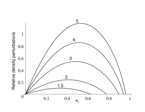
Figure 1: Relative density perturbations, $\langle\delta n^{2}\rangle^{1/2}/n_{0}$, vs. the ion magnetization parameter $\kappa_{i}\equiv\Omega_{i}/\nu_{i}$ for different values of $E_{0}/E_{\mathrm{Thr}}^{\min}$ (shown near the curves).

Figure 1 based on Eqs. (21) and (22) with $\alpha_{1}=1$ and $\chi_{\vec{k}}^{\mathrm{pr}}=0$ (Dimant and Milikh, 2003) shows that if $E_{0}/E_{\mathrm{Thr}}^{(0)}$ is large enough then relative rms density perturbations may even exceed unity. Such non-physical occasions break the validity of our quasilinear approximation. We should bear in mind, however, that large values of $E_{0}$ automatically lead to strong electron and ion temperature elevations due to combined regular and anomalous heating. This raises $E_{\mathrm{Thr}}^{(0)}\propto(T_{e}+T_{i})^{1/2}$ and prevents $E_{0}/E_{\mathrm{Thr}}^{(0)}$ from reaching too large values (we discuss this issue in more detail in the next section). For example, in the extreme case of $E_{0}=160\,$mV/m, the electron temperature reaches above $4000$ K (Bahcivan, 2007) at an altitude around 110 km corresponding to $\kappa_{i}\simeq 0.3$ (Dimant and Oppenheim, 2004, Fig. 2), not counting the simultaneously increasing ion temperature. According to Eq. (16), this raises $E_{\mathrm{Thr}}^{(0)}$ above $50\,$mV/m, making $E_{0}/E_{\mathrm{Thr}}^{(0)}<3$. We believe that this extreme value of $E_{0}/E_{\mathrm{Thr}}^{(0)}$ imposes the top restriction on possible density perturbations, keeping them below $50\%$. Less extreme but more typical density perturbations are expected to be largely within the reliable limits of the quasilinear approach.

Applying $\vec{k}/\vec{k}\simeq(\vec{k}/\vec{k})^{\mathrm{pr}}$, while replacing $(1+\psi_{\vec{k}}^{\mathrm{m}})$ according to Eq. (18) and $\langle\delta n^{2}\rangle^{1/2}$ according to Eq. (21), we use Eqs. (9) and (10) to express the turbulent conductivities in terms of the corresponding laminar conductivities given by Eq. (8) as

$$\sigma_{\mathrm{P}}^{\mathrm{NC}} \simeq\frac{\alpha_{1}\left[\left(1-\kappa_{i}^{2}\right)\cos\chi_{\vec{k}}-2\kappa_{i}\sin\chi_{\vec{k}}\right]\cos^{3}\chi_{\vec{k}}}{1+\kappa_{i}^{2}}$$

$$\times\left(\frac{E_{0}}{E_{\mathrm{Thr}}^{\min}}-1\right)\left(1-\frac{E_{\mathrm{Thr}}^{\min}}{E_{0}}\right)\sigma_{\mathrm{P}}^{\mathrm{L}},$$ (23a)

$$\sigma_{\mathrm{H}}^{\mathrm{NC}} \simeq-\ \frac{\alpha_{1}\left[2\kappa_{i}\cos\chi_{\vec{k}}+\left(1-\kappa_{i}^{2}\right)\sin\chi_{\vec{k}}\right](1+\psi_{\perp})\cos^{3}\chi_{\vec{k}}}{1+\kappa_{i}^{2}}$$

$$\times\left(\frac{E_{0}}{E_{\mathrm{Thr}}^{\min}}-1\right)\left(1-\frac{E_{\mathrm{Thr}}^{\min}}{E_{0}}\right)\sigma_{\mathrm{H}}^{\mathrm{L}}.$$ (23b)

These relations are only applicable for $E_{0}\geq E_{\mathrm{Thr}}^{\min}$ and $\kappa_{i}\leq 1$, otherwise $\sigma_{\mathrm{P,H}}^{\mathrm{NC}}=0$. Furthermore, according to Eqs. (15) and (16), the threshold field $E_{\mathrm{Thr}}^{\min}\propto E_{\mathrm{Thr}}^{(0)}\propto(T_{e}+T_{i})^{1/2}$ depends strongly on the electron and ion temperatures. This means that the self-consistent inclusion of the turbulent conductivity in the total conductivity tensor requires simultaneously including AEH (Dimant and Milikh, 2003; Milikh and Dimant, 2003), otherwise the effect of NC-induced turbulent conductivity will be exaggerated dramatically.

The AEH-induced increase in the plasma density due to the temperature reduction of the recombination rate (Dimant and Milikh, 2003; Milikh et al., 2006) will raise all values in the conductivity tensor in proportion to the increased plasma density. This slowly-developing effect, however, can slightly decrease if the strong external electric field $\vec{E}_{0}$ varies too fast (Codrescu et al., 1995, 2000; Matsuo and Richmond, 2008; Cosgrove et al., 2009; Cosgrove and Codrescu, 2009).

4 Turbulent Frictional Heating in Global Modeling

An accurate description of strong electric-field perturbations, such as storms, substorms, and sub-auroral polar streams, requires including macroscopic effects of E-region turbulence into global computer models, like the Coupled Magnetosphere Ionosphere Thermosphere (CMIT) model (Wiltberger et al., 2004; Wang et al., 2004). This model has been created by combining the magnetosphere MHD solver LFM (Lyon et al., 2004) and ionosphere-thermosphere NCAR solver TIEGCM (Roble and Ridley, 1994; Wang et al., 1999). The ring-current model RCM (Toffoletto et al., 2003) has been added recently, as well as TIEGCM has been extended to cover the mesosphere (TIMEGCM). Currently, the CMIT-RCM model includes ionospheric processes associated only with laminar conductivities. The turbulence-induced non-linear current (NC) can be incorporated by adding turbulent conductivities given by Eq (23). Self-consistency requires including also anomalous plasma heating caused by turbulent fields. The AEH increases (through the reduced recombination rate) the plasma density and, hence, all conductivities in proportion. However, the anomalous temperature elevations exert a negative feedback on the saturated level of the plasma turbulence, reducing the NC and its non-linear Pedersen conductivity.

Effects of E-region turbulence can be included directly in TIMEGCM and other codes that that model high-latitude neutral and plasma dynamics and chemical reactions. Given accurate heating sources, TIMEGCM includes all ionization/recombination and collisional cooling processes automatically. To account for temperature inputs caused by both laminar and turbulent fields, the energy balance equation for each species should include the corresponding source of frictional heating. Currently, TIMEGCM includes the laminar ion and neutral frictional heating but neglects the electron one. This is a reasonable approximation for altitudes above 100 km under quiet ionospheric conditions. However, during strong electric-field events, the E-region turbulence via AEH dramatically raises the electron temperature, meaning that the total electron frictional heating should also be included. For the convection field well above the instability threshold field given by Eqs. (23), ion turbulent heating can also be appreciable (for $E_{0}\gg E_{\mathrm{Thr}}^{\min}$, it is comparable to the ion laminar heating). Accuracy of the entire global model requires including the corresponding neutral frictional heating as well. Note that highly anisotropic E-region turbulence also causes average momentum changes in the plasma. Plasma-neutral collisions in turn can transfer these changes to neutral particles. For the weakly ionized E region, however, relative momentum changes are much less important than relative energy changes, so that we will ignore the former and focus entirely on the latter.

In the multi-component E-region ionosphere where electron-neutral (e-n) and ion-neutral (i-n) collisions dominate, we can calculate the total laminar and turbulent frictional heating of electrons, $H_{e}^{\mathrm{tot}}$, ions, $H_{i}^{\mathrm{tot}}$, and neutrals, $H_{n}^{\mathrm{tot}}$, using a quasilinear approximation to quadratic accuracy. In terms of the average turbulent perturbations, these are given by

$$H_{e}^{\mathrm{tot}} =m_{e}\nu_{e}\left[n_{0}\left(V_{e0}^{2}+\left\langle\delta V_{e}^{2}\right\rangle\right)+2(\vec{V}_{e0}\cdot\langle\delta n\delta\vec{V}_{e}\rangle)\right],$$

$$H_{i}^{\mathrm{tot}} =\sum_{n}\frac{m_{i}m_{n}\nu_{in}}{m_{i}+m_{n}}$$

$$\times\left[n_{i0}\left(V_{i0}^{2}+\left\langle\delta V_{i}^{2}\right\rangle\right)+2(\vec{V}_{i0}\cdot\langle\delta n_{i}\delta\vec{V}_{i}\rangle)\right],$$ (24)

$$H_{n}^{\mathrm{tot}} =\sum_{i}\frac{m_{i}^{2}\nu_{in}}{m_{i}+m_{n}}$$

$$\times\left[n_{i0}\left(V_{i0}^{2}+\left\langle\delta V_{i}^{2}\right\rangle\right)+2(\vec{V}_{i0}\cdot\langle\delta n_{i}\delta\vec{V}_{i}\rangle)\right],$$

with the summations taken over all possible collisions between ions and neutrals, where indices $i$ and $n$ refer to separate groups of ions or neutrals; $\sum_{i}n_{i0}=n_{0}$. The physical meaning of various terms in the square brackets is explained in Dimant and Oppenheim (2011). The expressions for $H_{i,n}^{\mathrm{tot}}$ explicitly take into account the fact that only $m_{n}/(m_{i}+m_{n})$ of the partial i-n electric field heating, $m_{i}\nu_{in}V_{i}^{2}$, goes to ions ($H_{i}^{\mathrm{tot}}$), while the remaining fraction goes directly to the colliding neutrals ($H_{n}^{\mathrm{tot}}$). The total electron collision frequency $\nu_{e}$ includes all electron-neutral (e-n) collisions, $\nu_{e}=\sum_{n}\nu_{en}$; but because $m_{e}\ll m_{n}$, the contributions to $H_{n}^{\mathrm{tot}}$ from the e-n collisions are negligible. Equation (24) is written in the neutral frame of reference, presuming that all thermosphere components move with a common neutral-wind velocity.

In a multi-fluid plasma, the laminar and turbulent velocities, $\vec{V}_{s0}$ and $\delta\vec{V}_{s}$, can be expressed in terms of the convection field $\vec{E}_{0}$ and spectral harmonics of the wave potential $\delta\Phi_{\vec{k},\omega}$ similarly to the two-fluid plasma (Dimant and Oppenheim, 2011). However, the first-order linear relations between the harmonics of the ion spectral densities, $\delta n_{i\vec{k},\omega}$, and potential, $\delta\Phi_{\vec{k},\omega}$, which are crucial for obtaining equations like Eq. (19), (43), can be rather complicated or cannot even be expressed in any closed analytical form. The reason is that the algebraic order of the underlying linear dispersion relation for the first-order wave frequency, $\omega_{\vec{k}}$, in the general case equals the number of separate ion species. Even for the two dominant E-region ion species, NO⁺ and O${}_{2}^{+}$, when the dispersion relation reduces to a quadratic equation, the first-order relations become cumbersome. These relations, however, simplify dramatically if all ion species have a common magnetization parameter, $\kappa_{i}=\Omega_{i}/\nu_{i}$ ($\nu_{i}\equiv\sum_{n}\nu_{in}$), so that all ion species respond to the fields equally. As a result, the multi-fluid relation between $\delta\Phi_{\vec{k},\omega}$ and $\delta n_{\vec{k},\omega}$ and various terms in $n_{s0}\left(V_{s0}^{2}+\left\langle\delta V_{s}^{2}\right\rangle\right)+2(\vec{V}_{s0}\cdot\langle\delta n_{s}\delta\vec{V}_{s}\rangle)$ ($s=e,i$) reduce to two-fluid Eqs. (49) and (51) from Dimant and Oppenheim (2011). For $\kappa_{e}\gg 1\gtrsim\kappa_{i}$, these become

$$\nu_{e}n_{0}V_{e0}^{2}\approx\frac{\nu_{e}n_{0}E_{0}^{2}}{B^{2}},\qquad\nu_{i}n_{i0}V_{i0}^{2}=\frac{\nu_{i}n_{i0}\kappa_{i}^{2}E_{0}^{2}}{\left(1+\kappa_{i}^{2}\right)B^{2}},$$ (25)

$$\nu_{e}n_{0}\left\langle\delta V_{e}^{2}\right\rangle \approx\frac{m_{i}\nu_{i}n_{0}(1+\kappa_{i}^{2})}{m_{e}}\sum_{\vec{k},\omega\neq 0}\frac{\psi_{\vec{k}}(\vec{k}\cdot\vec{U}_{0})^{2}}{(1+\psi_{\vec{k}})^{2}k_{\perp}^{2}}\left|\frac{\delta n_{\vec{k},\omega}}{n_{0}}\right|^{2},$$ (26a)

$$\nu_{i}n_{i0}\left\langle\delta V_{i}^{2}\right\rangle \approx\nu_{i}n_{i0}(1+\kappa_{i}^{2})\sum_{\vec{k},\omega\neq 0}\frac{(\vec{k}\cdot\vec{U}_{0})^{2}}{(1+\psi_{\vec{k}})^{2}k_{\perp}^{2}}\left|\frac{\delta n_{\vec{k},\omega}}{n_{0}}\right|^{2},$$ (26b)

$$2\nu_{e}(\vec{V}_{e0}\cdot\langle\delta n\delta\vec{V}_{e}\rangle) \approx\frac{2en_{0}(1+\kappa_{i}^{2})}{m_{e}\kappa_{i}\kappa_{e}}$$

$$\sum_{\vec{k},\omega\neq 0}\frac{(\vec{k}\cdot\vec{E}_{0})(\vec{k}\cdot\vec{U}_{0})}{(1+\psi_{\vec{k}})k_{\perp}^{2}}\left|\frac{\delta n_{\vec{k},\omega}}{n_{0}}\right|^{2},$$ (27a)

$$2\nu_{i}(\vec{V}_{i0}\cdot\langle\delta n_{i}\delta\vec{V}_{i}\rangle) \approx\frac{2en_{i0}}{m_{i}}\sum_{\vec{k},\omega\neq 0}\frac{(\vec{k}\cdot\vec{E}_{0})(\vec{k}\cdot\vec{U}_{0})}{(1+\psi_{\vec{k}})k_{\perp}^{2}}\left|\frac{\delta n_{\vec{k},\omega}}{n_{0}}\right|^{2}.$$ (27b)

where $$\delta n_{\vec{k},\omega}=\sum_{i}\delta n_{i\vec{k},\omega} \psi_{\vec{k}} \vec{U}_{0} (1+\kappa_{i}^{2})(1+\kappa_{e}^{2}k_{\parallel}^{2}/k_{\perp}^{2}) \psi_{\vec{k}}/\psi_{\perp}=\kappa_{e}\kappa_{i}\psi_{\vec{k}}$$ is the electron density, and are given by Eqs. (12) and (13), and emerging in the derivation of Eq. (26a) was approximated by (Dimant and Oppenheim, 2011, see Eq. (34b) and text below it).

To calculate heating rates in terms of E-region parameters, we need estimates of the turbulent density perturbations. Using the heuristic model of saturated turbulence, along with the approach that lead us from Eq. (9) via Eqs. (17), (18), and (21) to Eq. (23), we obtain

$$\sum_{\vec{k},\omega\neq 0}\frac{\psi_{\vec{k}}(\vec{k}\cdot\vec{U}_{0})^{2}}{(1+\psi_{\vec{k}})^{2}k_{\perp}^{2}}\left|\frac{\delta n_{\vec{k},\omega}}{n_{0}}\right|^{2}\simeq\frac{\alpha_{1}\kappa_{i}^{2}(E_{0}-E_{\mathrm{Thr}}^{\min})^{2}\cos^{4}\chi_{\vec{k}}^{\mathrm{pr}}}{(1+\kappa_{i}^{2})^{3}B^{2}}$$

$$\times\left[\frac{E_{0}}{E_{\mathrm{Thr}}^{\min}}\left(1+\psi_{\perp}\right)-1\right],$$

$$\sum_{\vec{k},\omega\neq 0}\frac{(\vec{k}\cdot\vec{U}_{0})^{2}}{(1+\psi_{\vec{k}})^{2}k_{\perp}^{2}}\left|\frac{\delta n_{\vec{k},\omega}}{n_{0}}\right|^{2}\simeq\frac{\alpha_{1}\kappa_{i}^{2}(E_{0}-E_{\mathrm{Thr}}^{\min})^{2}\cos^{4}\chi_{\vec{k}}^{\mathrm{pr}}}{(1+\kappa_{i}^{2})^{3}B^{2}},$$

$$\sum_{\vec{k},\omega\neq 0}\frac{(\vec{k}\cdot\vec{E}_{0})(\vec{k}\cdot\vec{U}_{0})}{(1+\psi_{\vec{k}})k_{\perp}^{2}}\left|\frac{\delta n_{\vec{k},\omega}}{n_{0}}\right|^{2}$$

$$\simeq\frac{\alpha_{1}\kappa_{i}^{2}(E_{\mathrm{Thr}}^{\min}-E_{0})^{2}\cos^{3}\chi_{\vec{k}}^{\mathrm{pr}}\sin\chi_{\vec{k}}^{\mathrm{pr}}}{(1+\kappa_{i}^{2})^{5/2}B}.$$ (28)

Equations (24)–(28) provide frictional heating terms for the potential inclusion into the corresponding energy-balance equations of TIMEGCM or similar ionosphere-thermosphere models. Equations (23)–(24) provide a reasonable estimate of turbulent conductivity and heating and should greatly improve modeling of the geospace environment during disturbed conditions.

5 Discussion

Figures 2–5 illustrate anomalous heating and give examples of the anomalously modified Pedersen conductivity for two cases: an extreme field of $150$ mV/m and a still large but more modest case of $80$ mV/m. These figures are based on typical high-latitude ionospheric parameters and the same values of the major HMT parameter, $\alpha_{1}=1$, as in Milikh and Dimant (2003). Figure 2 shows the effect of AEH and normal ion heating. The combined temperature, $T_{e}+T_{i}$, shows kinks at altitudes where AEH sharply disappears, while ion heating continues its steep rising. These altitudes are slightly below the ion magnetization boundary ($\kappa_{i}=1$) located at $h_{1}\simeq 122$ km. These kinks translate to those in the threshold electric field, $E_{\mathrm{Thr}}^{\min}\propto\ (T_{e}+T_{i})^{1/2}$, as seen in Fig. 3. Figure 3 (a) shows that above 100 km of altitude the threshold field increases dramatically due to plasma heating, keeping $E_{0}/E_{\mathrm{Thr}}^{\min}$ at a modest level of 2–3. The much weaker field of $E_{0}=80$ mV/m (b) gives a slightly lower ratio because the plasma heating in this case is also much lower. According to Fig. 1, such moderate ratio of $E_{0}/E_{\mathrm{Thr}}^{\min}$, even for the extreme case of $E_{0}=150$ mV/m, keeps the total density fluctuation level below 50%, i.e., roughly within the framework of the quasilinear approach (see above). This also reduces the entire effect of NC on the conductivity, as seen from Fig. 4.

Figure 4 shows a typical altitudinal profile of the undisturbed conductivity (curve 0) along with two curves including the anomalous conductivity. The NC effect alone (curve 1) nearly doubles the conductivity in a broad altitude range between 90 km and the ion magnetization boundary located at an altitude $h_{1}\simeq 122$ km, fairly close to the maximum of the normal Pedersen conductivity. The AEH-induced ionization-recombination effect doubles the total conductivity once again (curve 2), but this occurs in a slightly narrower range restricted from above by the AEH upper boundary, $h_{0}\simeq 119.5$ km. Presuming that the lower altitudes located below the undisturbed conductivity maximum near $h_{1}$ include about a half of the entire height-integrated conductance, we see that the NC-induced anomalous conductivity alone (curve 1) can contribute up to a half of the undisturbed conductance, while both anomalous effects combined (curve 2) can nearly double the entire conductance. We should bear in mind, however, the caveats associated with slow evolution of ionization-recombination processes superposed on rapidly varying electric field (see the discussion above).

Largely the same situation takes place for the smaller field of $E_{0}=80$ mV/m (Fig. 5). Since in this case the particle-temperature elevation is more modest than that for $E_{0}=150$ mV/m, the instability threshold field shown in Figure 3 (b) remains noticeably lower than that in Fig. 3 (a). As a result, the ratio $E_{0}/E_{\mathrm{Thr}}^{\min}$ changes much less dramatically compared to $E_{0}=150$ mV/m. That is why in Fig. 5 the NC-induced effect for $E_{0}=80$ mV/m turns out to be nearly as strong as that in Fig. 4 for $E_{0}=150$ mV/m, while the more fragile AEH-induced recombination effect is much less pronounced because of lower electron heating.

Above we presumed a rather conservative value for the major HMT parameter, $\alpha_{1}=1$, the same as in Dimant and Milikh (2003); Milikh and Dimant (2003); Merkin et al. (2005b); Milikh et al. (2006). Recent 2D and 3D PIC simulations (Oppenheim et al., 2011) suggest that $\alpha_{1}$ can actually be closer to $1.5$. This would make $\sigma_{\mathrm{P}}^{\mathrm{NC}}/\sigma_{\mathrm{P}}^{\mathrm{L}}$ roughly 50% larger, although due to larger $\langle\delta n^{2}\rangle^{1/2}/n_{0}$ one may have stronger restrictions on the quasilinear approach. We should also note that our current heuristic model of developed turbulence does not include the ion thermal driving mechanism (ITM) (Dimant and Oppenheim, 2004; Oppenheim and Dimant, 2004).

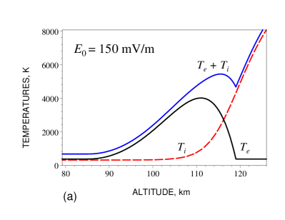
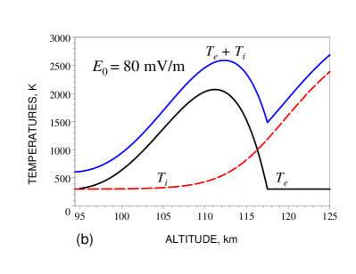
Figure 2: Altitude dependence of the electron and ion temperatures, $T_{e}$ and $T_{i}$, for two different values of $E_{0}$ (shown in figures). The electron temperature includes self-consistent AEH according to Milikh and Dimant (2003). The kinks in $T_{e}$ and $T_{e}+T_{i}$ near the 119.5 km altitude (a) and 117.5 km (b) are caused by sharp disappearance of instability and, hence, AEH.

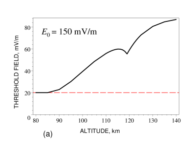
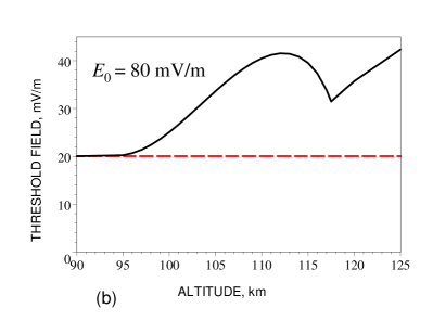
Figure 3: Altitude dependence of the FB-instability threshold electric field, $E_{\mathrm{Thr}}^{\min}$, Eqs. (15) and (16), elevated due to particle heating for the same values $E_{0}$ as in Fig. 2. The kinks in $E_{\mathrm{Thr}}^{\min}\propto(T_{e}+T_{i})^{1/2}$ correspond to those in Fig. 2.

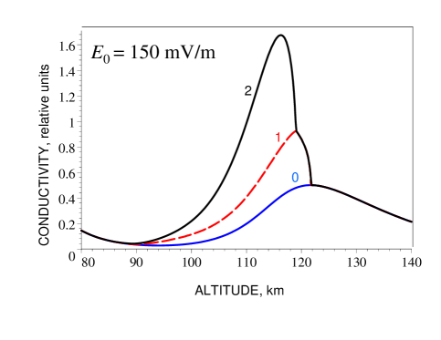
Figure 4: Altitude dependence of the total – normal and anomalous – Pedersen conductivity for $E_{0}=150$ mV/m (in relative units). Curve 0 shows the undisturbed conductivity. Curve 1 includes additionally the NC-induced anomalous conductivity calculated according to Eq. (23a) with $\alpha_{1}=0$ and $\chi_{\vec{k}}=0$. Curve 2 shows the total Pedersen conductivity with the AEH-affected plasma density elevated according to the steady-state ionization recombination model by Milikh et al. (2006). The NC-induced anomalous conductivity disappears above the ion magnetization boundary $\simeq 122$ km; the AEH-recombination effect vanishes above the top boundary of anomalous heating $\simeq 119.5$ km (see the corresponding kinks in Figs. 2 and 3).

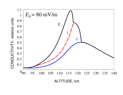
Figure 5: The same as Fig. 4, but for $E_{0}=80$ mV/m.

That is why all our anomalous effects occur strictly below the ion magnetization boundary, $\kappa_{i}=1$. Possible inclusion of the ITM would play a two-fold role. On the one hand, this would expand the altitudinal range of anomalous conductivity to at least a few kilometers higher (Dimant and Oppenheim, 2004) and increase the total ionospheric conductance accordingly. A modest reduction in $\kappa_{i}$ due to anomalously heated ions might also help. On the other hand, near the ion magnetization boundary the preferred values of the modified flow angle $\chi_{\vec{k}}$ deviate from $\chi_{\vec{k}}=0$, also due to the ITM as explained in Dimant and Oppenheim (2004). This deviation of $\chi_{\vec{k}}$ would slightly reduce the $\chi_{\vec{k}},\kappa_{i}$-dependent factor in the RHS of Eq. (23a) and hence lead to a smaller Pedersen conductivity compared to that for $\chi_{\vec{k}}=0$. An accurate inclusion of the ITM to the heuristic model of saturated turbulence, however, would complicate the entire model. We plan to improve the treatment of the top electrojet altitudes in future by using both analytical theory and PIC simulations. At this moment, a better accuracy is of less importance than the mere fact that the instability-induced conductivity occupies roughly the entire lower half of the Pedersen conductive layer and can nearly double the whole conductance. Note also that polarized sporadic-E clouds (Dimant and Oppenheim, 2010), or even ubiquitous meteor trails (Dimant et al., 2009), can also make additional contributions to anomalous conductances. All these effects combined can, at least partially, explain why global MHD codes developed for predictive modeling of space weather which use normal conductances often overestimate the cross-polar cap potentials by close to a factor of two.

6 Summary and Conclusions

Plasma turbulence generated by E-region instabilities significantly modifies the ionospheric Pedersen conductance by exciting a net non-linear current, $\vec{j}^{\mathrm{NC}}=\overleftrightarrow{\sigma_{\mathrm{P}}^{\mathrm{NC}}}\cdot\vec{E}_{0}$. The magnitude of $\vec{j}^{\mathrm{NC}}$ can only be a fraction of the undisturbed Hall current, but can be comparable in magnitude to the Pedersen current and pointing in that direction. This creates an additional turbulent conductivity. Also, anomalous electron heating, via reduced plasma recombination, increases the mean plasma density $n_{0}$ and all, laminar and turbulent, conductances in proportion with $n_{0}$. Estimates based on a quasilinear theory and heuristic model of non-linearly saturated plasma turbulence show that the anomalous effects combined can nearly double the Pedersen conductance, as predicted by Eqs. (9) and (23) and illustrated by Figs. 4 and 5. Such ionospheric response to the magnetospheric field $\vec{E}_{0}$ may efficiently reduce the high-latitude ionospheric resistance and decrease the cross-polar cap potential. This effect might explain, at least partially, why routine MHD simulations with the normal ionospheric conductances systematically overestimate this potential by a factor of two. The anomalous effects on the conductances, as well as turbulent frictional heating, should be included in global MHD codes developed for space weather prediction.

Appendix: General FB/GD Dispersion Relation for Arbitrarily Magnetized Plasmas

This appendix develops the two-fluid linear theory of the Farley-Buneman (FB) and gradient drift (GD) instabilities for arbitrary magnetization parameters, $\kappa_{e,i}\equiv\Omega_{e,i}/\nu_{e,i}$, that vary from small values at lower altitudes to large values at higher altitudes. This analysis has never been published but is relevant to the lower ionosphere and enables one to accurately estimate conventionally neglected terms that may matter in some cases.

The approach described below allows one to obtain the fluid-model dispersion relation in a reasonably compact and physically clear way. Compared to Sect. 3.1 of Dimant and Oppenheim (2011), here we additionally include the particle pressure, inertia, regular gradients in the background plasma density, and recombination. These factors are responsible for the FB and GD instability drivers, as well as for the stabilizing diffusion and ionization balance. For simplicity, we do not include non-isothermal processes responsible for driving of thermal instabilities (Dimant and Sudan, 1997; Kagan and Kelley, 2000; Dimant and Oppenheim, 2004) and ignore the stabilizing effect of a weak non-quasineutrality (Rosenberg and Chow, 1998; Kovalev et al., 2008). These factors can be added using essentially the same approach.

The quasineutral two-fluid continuity equations including ionization and recombination balance are

$$\partial_{t}n+\nabla\cdot(n\vec{V}_{e})=\partial_{t}n+\nabla\cdot(n\vec{V}_{i})=Q-\alpha n^{2},$$ (29)

where $Q$ is the total source of ionization and $\alpha$ is the recombination constant. Equation (29) includes the standard quasineutral relation $\nabla\cdot(n\vec{U})=0$, where $\vec{U}\equiv\vec{V}_{e}-\vec{V}_{i}$.

The continuity equations for a stationary ($\partial_{t}n_{0}=0$) but inhomogeneous background density, $n_{0}$, with the corresponding undisturbed fluid velocities, $\vec{V}_{e,i0}$, are

$$\nabla\cdot(n_{0}\vec{V}_{e0})=\nabla\cdot(n_{0}\vec{V}_{i0})=Q-\alpha_{0}n_{0}^{2}.$$ (30)

From the left equality, the divergence of the relative velocity, $\vec{U}_{0}\equiv\vec{V}_{e0}-\vec{V}_{i0}$, can be expressed in terms of the background density gradient as

$$\nabla\cdot\vec{U}_{0}=-\vec{U}_{0}\cdot\nabla n_{0}/n_{0}.$$ (31)

In what follows, we presume that both $\vec{U}_{0}$ and $n_{0}$ are known functions of spatial coordinates that satisfy Eq. (31). Then, to express the zero-order drift velocities of electrons and ions in terms of $\vec{U}_{0}$, we can use Eqs. (26) and (27) from Dimant and Oppenheim (2011) to obtain

$$\vec{V}_{e0\parallel}=\frac{\kappa_{e}\vec{U}_{0\parallel}}{\kappa_{e}+\kappa_{i}},\qquad\vec{V}_{i0\parallel}=-\ \frac{\kappa_{i}\vec{U}_{0\parallel}}{\kappa_{e}+\kappa_{i}},$$ (32)

$$\vec{V}_{e0\perp} =\frac{\kappa_{e}[\vec{U}_{0\perp}-\kappa_{i}(\vec{U}_{0}\times\hat{b})]}{\kappa_{e}+\kappa_{i}},$$ (33a)

$$\vec{V}_{i0\perp} =-\ \frac{\kappa_{i}[\vec{U}_{0\perp}+\kappa_{e}(\vec{U}_{0}\times\hat{b})]}{\kappa_{e}+\kappa_{i}}.$$ (33b)

Note that these expressions are only valid when neglecting for the background plasma pressure gradients and gravity, comparably small effects for almost all ionospheric conditions.

We will now consider Fourier harmonics of wave perturbations, $\delta n_{\vec{k}}$, $\delta\vec{E}_{\vec{k}}$, $\delta\vec{V}_{e,i\vec{k}}\propto\exp[i(\vec{k}\cdot\vec{r}-\omega_{\vec{k}}t)]$, where the wavevector $\vec{k}$ and the complex linear wave frequency, $\omega_{\vec{k}}=\omega_{\vec{k}}^{\prime}+i\gamma_{\vec{k}}$, are locally defined. Here $\omega_{\vec{k}}^{\prime}$ is the real wave frequency, while $\gamma_{\vec{k}}\equiv-i\operatorname{Im}\,\omega_{\vec{k}}$ is the wave total growth or damping rate.

Linearizing Eq. (30) with respect to $\delta n_{\vec{k}}$, $\delta\vec{V}_{e,i\vec{k}}$ and introducing two shifted complex wave frequencies,

$$\Omega_{\vec{k}}^{(e)} \equiv\omega_{\vec{k}}-\hat{K}\cdot\vec{V}_{e0}+2i\alpha n_{0},$$ (34a)

$$\Omega_{\vec{k}}^{(i)} \equiv\omega_{\vec{k}}-\hat{K}\cdot\vec{V}_{i0}+2i\alpha n_{0}=\Omega_{\vec{k}}^{(e)}+q,$$ (34b)

with

$$\hat{K}\equiv\vec{k}-i\nabla,\qquad q\equiv\hat{K}\cdot\vec{U}_{0},$$ (35)

we obtain

$$\Omega_{\vec{k}}^{(e)}\ \frac{\delta n_{\vec{k}}}{n_{0}}=\vec{p}\cdot\delta\vec{V}_{e\vec{k}},\qquad\Omega_{\vec{k}}^{(i)}\ \frac{\delta n_{\vec{k}}}{n_{0}}=\vec{p}\cdot\delta\vec{V}_{i\vec{k}},$$ (36)

where

$$\vec{p}\equiv\frac{\vec{K}n_{0}}{n_{0}}=\vec{k}-\frac{i\nabla n_{0}}{n_{0}}.$$ (37)

Now we express $\delta\vec{V}_{e,i\vec{k}}$ in terms of $\delta n_{\vec{k}}$ and $\delta\Phi_{\vec{k},\omega}$, $\delta\vec{E}_{\vec{k}}=-i\vec{k}\delta\Phi_{\vec{k},\omega}$, using the momentum equations for the individual electron and ion mean fluid velocities in the neutral frame,

$$m_{e}\ \frac{\mathrm{d}_{e}\vec{V}_{e}}{\mathrm{d}t} =-e(\vec{E}+\vec{V}_{e}\times\vec{B})-\frac{\nabla\left(nT_{e}\right)}{n}-m_{e}\nu_{e}\vec{V}_{e},$$ (38a)

$$m_{i}\ \frac{\mathrm{d}_{i}\vec{V}_{i}}{\mathrm{d}t} =e(\vec{E}+\vec{V}_{i}\times\vec{B})-\frac{\nabla\left(nT_{i}\right)}{n}-m_{i}\nu_{i}\vec{V}_{i},$$ (38b)

where $\mathrm{d}_{e,i}/\mathrm{d}t\equiv\partial_{t}+\vec{V}_{e,i}\cdot\nabla$ are the full derivatives for both electrons and ions. For low-frequency E/D-region plasma processes, the electron inertia described by the LHS of Eq. (38a), unlike the ion inertia in Eq. (38b), is usually neglected, but we will keep it for completeness and symmetry. Neglecting in Eq. (38) temperature perturbations, we express the velocity perturbations as

$$\delta\vec{V}_{e\vec{k}} =\vec{G}_{e}\left(\delta\Phi_{\vec{k},\omega}-\frac{T_{e}}{e}\ \frac{\delta n_{\vec{k}}}{n_{0}}\right),$$ (39a)

$$\delta\vec{V}_{i\vec{k}} =\vec{G}_{i}\left(\delta\Phi_{\vec{k},\omega}+\frac{T_{i}}{e}\ \frac{\delta n_{\vec{k}}}{n_{0}}\right),$$ (39b)

where the vector-functions $\vec{G}_{e,i}$,

$$\vec{G}_{e\parallel} \approx\frac{i\tilde{\kappa}_{e}\vec{k}_{\parallel}}{B},\qquad\vec{G}_{e\perp}\approx\frac{i\tilde{\kappa}_{e}(\vec{k}_{\perp}-\tilde{\kappa}_{e}\vec{k}\times\hat{b})}{\left(1+\tilde{\kappa}_{e}^{2}\right)B},$$ (40a)

$$\vec{G}_{i\parallel} \approx-\ \frac{i\tilde{\kappa}_{i}\vec{k}_{\parallel}}{B},\qquad\vec{G}_{i\perp}\approx-\ \frac{i\tilde{\kappa}_{i}(\vec{k}_{\perp}+\tilde{\kappa}_{i}\vec{k}\times\hat{b})}{\left(1+\tilde{\kappa}_{i}^{2}\right)B},$$ (40b)

describe anisotropic two-fluid responses to the harmonic perturbations of the potential and pressures combined. Here, in accord with Eq. (45b),

$$\tilde{\kappa}_{e} \equiv\frac{\Omega_{e}}{\nu_{e}-i\Omega_{\vec{k}}^{(e)}}\approx\kappa_{e}\left(1+\frac{i\Omega_{\vec{k}1}^{(e)}}{\nu_{e}}\right),$$ (41a)

$$\tilde{\kappa}_{i} \equiv\frac{\Omega_{i}}{\nu_{i}-i\Omega_{\vec{k}}^{(i)}}\approx\kappa_{i}\left(1+\frac{i\Omega_{\vec{k}1}^{(i)}}{\nu_{i}}\right)$$ (41b)

are modified magnetization ratios that include small contributions from the particle inertia; $\Omega_{\vec{k}1}^{(e,i)}=\operatorname{Re}\Omega_{\vec{k}}^{(e,i)}=\omega_{\vec{k}}-\vec{k}\cdot\vec{V}_{e,i0}$. The small ion inertia contribution described by $i\Omega_{\vec{k}1}^{(,i)}/\nu_{i}$ is crucial for excitation of the FB instability.

Now we substitute the expressions for $\delta\vec{V}_{e,i\vec{k}}$ from Eq. (39) to Eq. (36), expressing $\Omega_{\vec{k}}^{(e)}=\Omega_{\vec{k}}^{(i)}-q$ via $q=\vec{k}\cdot\vec{U}_{0}-i\nabla\cdot\vec{U}_{0}=\vec{U}_{0}\cdot(\vec{p})^{\ast}$, where we used Eq. (31) and (35). This yields two independent linear relations between $\delta n_{\vec{k}}$ and $\delta\Phi_{\vec{k},\omega}$:

$$\left[\Omega_{\vec{k}}^{(e)}+\frac{T_{e}}{e}(\vec{p}\cdot\vec{G}_{e})\right]\frac{\delta n_{\vec{k}}}{n_{0}} =(\vec{p}\cdot\vec{G}_{e})\delta\Phi_{\vec{k},\omega},$$

$$\left[\Omega_{\vec{k}}^{(e)}+q-\frac{T_{i}}{e}(\vec{p}\cdot\vec{G}_{i})\right]\frac{\delta n_{\vec{k}}}{n_{0}} =(\vec{p}\cdot\vec{G}_{i})\delta\Phi_{\vec{k},\omega}.$$

From these relations and Eq. (34b), we obtain two symmetric expressions for the coupled shifted frequencies,

$$\Omega_{\vec{k}}^{(e)} =-\ \frac{(\vec{p}\cdot\vec{G}_{e})[q-(\vec{p}\cdot\vec{G}_{i})\left(T_{e}+T_{i}\right)/e]}{\vec{p}\cdot(\vec{G}_{e}-\vec{G}_{i})},$$ (42a)

$$\Omega_{\vec{k}}^{(i)} =-\ \frac{(\vec{p}\cdot\vec{G}_{i})[q-(\vec{p}\cdot\vec{G}_{e})\left(T_{e}+T_{i}\right)/e]}{\vec{p}\cdot(\vec{G}_{e}-\vec{G}_{i})},$$ (42b)

and the general relation between harmonics $\delta\Phi_{\vec{k},\omega}$ and $\delta n_{\vec{k}}$,

$$\delta\Phi_{\vec{k},\omega}=-\ \frac{q-\vec{p}\cdot(\vec{G}_{e}T_{e}+\vec{G}_{i}T_{i})/e}{\vec{p}\cdot(\vec{G}_{e}-\vec{G}_{i})}\ \frac{\delta n_{\vec{k}}}{n_{0}}.$$ (43)

Using the definitions of $\Omega_{\vec{k}}^{(e)}$ or $\Omega_{\vec{k}}^{(i)}$ given by Eq. (34), we obtain the complex wave frequency in the neutral frame, $\omega_{\vec{k}}=\Omega_{\vec{k}}^{(e)}+\hat{K}\cdot\vec{V}_{e0}-2i\alpha n_{0}=\Omega_{\vec{k}}^{(i)}+\hat{K}\cdot\vec{V}_{i0}-2i\alpha n_{0}$,

$$\omega_{\vec{k}}\equiv\omega_{\vec{k}}^{\prime}+i\gamma_{\vec{k}}=\frac{(\vec{p}\cdot\vec{G}_{e})(\hat{K}\cdot\vec{V}_{i0})-(\vec{p}\cdot\vec{G}_{i})(\hat{K}\cdot\vec{V}_{e0})}{\vec{p}\cdot(\vec{G}_{e}-\vec{G}_{i})}$$

$$+\frac{(\vec{p}\cdot\vec{G}_{i})(\vec{p}\cdot\vec{G}_{e})(T_{e}+T_{i})}{\vec{p}\cdot(\vec{G}_{e}-\vec{G}_{i})e}-2i\alpha n_{0}.$$ (44)

Equations (42) to (44) give the general expressions for the complex wave frequencies. To find the combined linear growth of instabilities or wave dissipation, $\gamma_{\vec{k}}=-i\,\operatorname{Im}\omega_{\vec{k}}$, they should be further split into the real and imaginary parts.

The approximate two-fluid description of local quasi-harmonic waves is valid provided the characteristic wavevectors and frequencies satisfy

$$L_{\parallel,\perp}^{-1}\ll k_{\parallel,\perp}\ll l_{e,i}^{-1},\rho_{e,i}^{-1},$$ (45a)

$$T^{-1},|\gamma_{\vec{k}}|\ll|\omega_{\vec{k}}^{\prime}|\ll\nu_{e,i}.$$ (45b)

Here $l_{e,i}$ are the typical mean free paths of the corresponding particles with respect to ion-neutral and electron-neutral collisions, $\rho_{e,i}$ are the gyroradii (if the corresponding particles are magnetized), and $T$ and $L_{\parallel,\perp}$ are typical temporal and spatial (parallel and perpendicular to $\vec{B}_{0}$) scales of ionospheric density variation. Equation (45a) should be satisfied separately for the parallel and perpendicular directions. Assuming these conditions, we will treat the wave pressure gradients, local gradients in the background density, and particle inertia as second-order effects with respect to the small parameters defined by Eq. (45). In this treatment, the first-order factors discussed in Dimant and Oppenheim (2011) define the real wave frequency, $\omega_{\vec{k}}^{\prime}$, while all second-order factors combined define the total linear damping or growth rate, $\gamma_{\vec{k}}$.

Under conditions specified by Eq. (45), the dominant real part of the wave frequency, $\omega_{\vec{k}}^{\prime}$, is determined by the first-order accuracy, $\omega_{\vec{k}}^{\prime}\approx\omega_{\vec{k}1}$, when neglecting the pressure gradients, particle inertia, regular gradients of the background plasma density, and recombination. To this accuracy, we have $\hat{K}\approx\vec{p}\approx\vec{k}$, $q\approx\vec{k}\cdot\vec{U}_{0}$, $\tilde{\kappa}_{e,i}=\kappa_{e,i}$, and hence

$$\vec{G}_{e\parallel} \approx\vec{G}_{e1\parallel}=\frac{i\kappa_{e}\vec{k}_{\parallel}}{B},\ \ \ \ \vec{G}_{e\perp}\approx\vec{G}_{e1\perp}=\frac{i\kappa_{e}(\vec{k}_{\perp}-\kappa_{e}\vec{k}\times\hat{b})}{\left(1+\kappa_{e}^{2}\right)B},$$ (46a)

$$\vec{G}_{i\parallel} \approx\vec{G}_{i1\parallel}=-\ \frac{i\kappa_{i}\vec{k}_{\parallel}}{B},\ \,\vec{G}_{i\perp}\approx\vec{G}_{i1\perp}=-\ \frac{i\kappa_{i}(\vec{k}_{\perp}+\kappa_{i}\vec{k}\times\hat{b})}{\left(1+\kappa_{i}^{2}\right)B},$$ (46b)

$$\vec{p}\cdot\vec{G}_{e} \approx\vec{k}\cdot\vec{G}_{e1}=\frac{i\kappa_{e}k_{\perp}^{2}}{(1+\kappa_{e}^{2})B}\left[1+(1+\kappa_{e}^{2})\frac{k_{\parallel}^{2}}{k_{\perp}^{2}}\right],$$

$$\vec{p}\cdot\vec{G}_{i} \approx\vec{k}\cdot\vec{G}_{i1}=-\ \frac{i\kappa_{i}k_{\perp}^{2}}{(1+\kappa_{i}^{2})B}\left[1+(1+\kappa_{i}^{2})\frac{k_{\parallel}^{2}}{k_{\perp}^{2}}\right].$$ (47)

Using Eqs. (12), we obtain

$$\vec{p}\cdot(\vec{G}_{e}-\vec{G}_{i})\approx\vec{k}\cdot(\vec{G}_{e1}-\vec{G}_{i1})=\frac{i\kappa_{i}\kappa_{e}\left(\kappa_{e}+\kappa_{i}\right)\left(1+\psi_{\vec{k}}\right)k_{\perp}^{2}}{\left(1+\kappa_{e}^{2}\right)\left(1+\kappa_{i}^{2}\right)B},$$ (48)

After neglecting small terms proportional to $\left(T_{e}+T_{i}\right)$ and $\alpha n_{0}$, Eq. (44) yields

$$\omega_{\vec{k}}\approx\omega_{\vec{k}1}=\frac{(\vec{k}\cdot\vec{G}_{e1})(\vec{k}\cdot\vec{V}_{i0})-(\vec{k}\cdot\vec{G}_{i1})(\vec{k}\cdot\vec{V}_{e0})}{\vec{k}\cdot(\vec{G}_{e1}-\vec{G}_{i1})}$$

and reduces to Eq. (37) from Dimant and Oppenheim (2011) with the corresponding real shifted frequencies, $\Omega_{\vec{k}1}^{(e,i)}\equiv\operatorname{Re}\Omega_{\vec{k}}^{(e,i)}=\omega_{\vec{k}1}-\vec{k}\cdot\vec{V}_{e,i0}$,

$$\Omega_{\vec{k}1}^{(e)}=-\ \frac{(\vec{k}\cdot\vec{U}_{0})(\vec{k}\cdot\vec{G}_{e1})}{\vec{k}\cdot(\vec{G}_{e1}-\vec{G}_{i1})},\qquad\Omega_{\vec{k}1}^{(i)}=-\ \frac{(\vec{k}\cdot\vec{U}_{0})(\vec{k}\cdot\vec{G}_{i1})}{\vec{k}\cdot(\vec{G}_{e1}-\vec{G}_{i1})},$$ (49)

given explicitly by the companion paper Eqs. (36) and (39).

Now we will develop the dispersion relationships to the second-order accuracy by taking into account all previously neglected factors: the wave pressure gradients, particle inertia, gradients of the zero-order plasma parameters, and recombination. All second-order terms in Eq. (44), representing linear corrections to the first-order real frequency $\omega_{\vec{k}1}$, are purely imaginary, so that their linear combination determines the total linear growth/damping rate, $\gamma_{\vec{k}}$.

We start by discussing the two last terms in the RHS of Eq. (44). The second-order term proportional to $(T_{e}+T_{i})$ originates from perturbations of the particle fluid pressure. To the leading-order accuracy, the term

$$\frac{(\vec{p}\cdot\vec{G}_{i})(\vec{p}\cdot\vec{G}_{e})(T_{e}+T_{i})}{\vec{p}\cdot(\vec{G}_{e}-\vec{G}_{i})e}\approx\frac{(\vec{k}\cdot\vec{G}_{i1})(\vec{k}\cdot\vec{G}_{e1})(T_{e}+T_{i})}{\vec{k}\cdot(\vec{G}_{e1}-\vec{G}_{i1})e}$$

$$=-\ \frac{ik_{\perp}^{2}\left[1+(1+\kappa_{e}^{2})k_{\parallel}^{2}/k_{\perp}^{2}\right]\left[1+(1+\kappa_{i}^{2})k_{\parallel}^{2}/k_{\perp}^{2}\right](T_{e}+T_{i})}{(\kappa_{e}+\kappa_{i})(1+\psi_{\vec{k}})eB}$$ (50)

contributes directly to $\gamma_{\vec{k}}$. The combination of the last two terms describes the major linear wave dissipation due to particle diffusion and recombination. For fully magnetized electrons, $\kappa_{e}\equiv\Omega_{e}/\nu_{e}\gg 1$, and unmagnetized ions, $\kappa_{i}\equiv\Omega_{i}/\nu_{i}\ll 1$, Eq. (50) reduces to the conventional loss term,

$$\frac{(\vec{p}\cdot\vec{G}_{i})(\vec{p}\cdot\vec{G}_{e})(T_{e}+T_{i})}{\vec{p}\cdot(\vec{G}_{e}-\vec{G}_{i})e}\approx-\ \frac{i\psi_{\vec{k}}k_{\perp}^{2}C_{s}^{2}}{(1+\psi_{\vec{k}})\nu_{i}},$$

where in this limit $\psi_{\vec{k}}\approx(1+\kappa_{e}^{2}k_{\parallel}^{2}/k_{\perp}^{2})\nu_{e}\nu_{i}/(\Omega_{e}\Omega_{i})$.

The first term in the RHS of Eq. (44) includes the major instability drivers. Unlike the two last terms, to the leading accuracy it is a first-order term. To retrieve second-order corrections, we have to linearize it with respect to small perturbations $\propto i\Omega_{\vec{k}}^{(e,i)}/\nu_{e,i}$ and $i\nabla$. Denoting the corresponding linear corrections by $\delta(\cdots)$, we have

$$\delta\left[\frac{(\vec{p}\cdot\vec{G}_{e})(\hat{K}\cdot\vec{V}_{i0})-(\vec{p}\cdot\vec{G}_{i})(\hat{K}\cdot\vec{V}_{e0})}{\vec{p}\cdot(\vec{G}_{e}-\vec{G}_{i})}\right]$$

$$\approx(\vec{k}\cdot\vec{V}_{i0})\delta\left[\frac{\vec{p}\cdot\vec{G}_{e}}{\vec{p}\cdot(\vec{G}_{e}-\vec{G}_{i})}\right]-(\vec{k}\cdot\vec{V}_{e0})\delta\left[\frac{\vec{p}\cdot\vec{G}_{i}}{\vec{p}\cdot(\vec{G}_{e}-\vec{G}_{i})}\right]$$

$$+\frac{(\vec{k}\cdot\vec{G}_{e1})(\delta\hat{K}\cdot\vec{V}_{i0})-(\vec{k}\cdot\vec{G}_{e1})(\delta\hat{K}\cdot\vec{V}_{i0})}{\vec{k}\cdot(\vec{G}_{e1}-\vec{G}_{i1})}.$$ (51)

According to Eq. (35), in the last term of Eq. (51) we have $\delta\hat{K}=-i\nabla$. Presuming a uniform magnetic field, $\vec{B}=B\hat{b}$, expressing $\vec{V}_{e,i0}$ in terms of $\vec{U}_{0}$ according to Eqs. (32), (33), and using Eqs. (47), (48), we obtain

$$\frac{(\vec{k}\cdot\vec{G}_{e1})(\delta\hat{K}\cdot\vec{V}_{i0})-(\vec{k}\cdot\vec{G}_{e1})(\delta\hat{K}\cdot\vec{V}_{i0})}{\vec{k}\cdot(\vec{G}_{e1}-\vec{G}_{i1})}$$

$$=\frac{i}{\kappa_{e}+\kappa_{i}}\left[\frac{(\kappa_{i}-\kappa_{e})\nabla\cdot\vec{U}_{0}}{1+\psi_{k}}+\kappa_{e}\kappa_{i}\hat{b}\cdot(\nabla\times\vec{U}_{0})\right].$$ (52)

Recall that $\nabla\cdot\vec{U}_{0}$ can be expressed in terms of $\nabla n_{0}$ according to Eq. (31). In this sense, the term proportional to $\nabla\cdot\vec{U}_{0}$ can be considered as an additional small contributor to the GD instability driving. The last vortex term $\propto\nabla\times\vec{U}_{0}$ is unrelated to any density gradients, but it may also contribute to $\gamma_{\vec{k}}$.

Next we turn to the combination of the two first terms in the RHS of Eq. (51). The difference between the two fractions $\left.\vec{p}\cdot\vec{G}_{e}\right/\vec{p}\cdot(\vec{G}_{e}-\vec{G}_{i})$ and $\left.\vec{p}\cdot\vec{G}_{i}\right/\vec{p}\cdot(\vec{G}_{e}-\vec{G}_{i})$ equals a constant value of $1$, so that their linear perturbations are equal and we have

$$(\vec{k}\cdot\vec{V}_{i0})\ \delta\left[\frac{\vec{p}\cdot\vec{G}_{e}}{\vec{p}\cdot(\vec{G}_{e}-\vec{G}_{i})}\right]$$ (53a)

$$- (\vec{k}\cdot\vec{V}_{e0})\ \delta\left[\frac{\vec{p}\cdot\vec{G}_{i}}{\vec{p}\cdot(\vec{G}_{e}-\vec{G}_{i})}\right]=-\beta(\vec{k}\cdot\vec{U}_{0}),$$

where

$$\beta \equiv\delta\left[\frac{\vec{p}\cdot\vec{G}_{e}}{\vec{p}\cdot(\vec{G}_{e}-\vec{G}_{i})}\right]=\delta\left[\frac{\vec{p}\cdot\vec{G}_{i}}{\vec{p}\cdot(\vec{G}_{e}-\vec{G}_{i})}\right]=\beta_{\mathrm{FB}}+\beta_{\mathrm{GD}},$$ (54a)

$$\beta_{\mathrm{FB}} \approx\frac{(\vec{k}\cdot\vec{G}_{e1})(\vec{k}\cdot\delta\vec{G}_{i})-(\vec{k}\cdot\vec{G}_{i1})(\vec{k}\cdot\delta\vec{G}_{e})}{[\vec{k}\cdot(\vec{G}_{e1}-\vec{G}_{i1})]^{2}},$$ (54b)

$$\beta_{\mathrm{GD}} \approx\frac{(\vec{k}\cdot\vec{G}_{e1})(\vec{G}_{i1}\cdot\delta\vec{p})-(\vec{k}\cdot\vec{G}_{i1})(\vec{G}_{e1}\cdot\delta\vec{p})}{[\vec{k}\cdot(\vec{G}_{e1}-\vec{G}_{i1})]^{2}}.$$ (54c)

Here the coefficient $\beta_{\mathrm{FB}}$ includes particle-inertia contributions responsible for the FB instability, while $\beta_{\mathrm{GD}}$ includes the background density gradients responsible for the GD instability.

First, we calculate the FB-instability driving term, $-\beta_{\mathrm{FB}}(\vec{k}\cdot\vec{U}_{0})$. According to Eqs. (40) and Eq. (41), we obtain

$$\vec{k}\cdot\delta\vec{G}_{e} =-\ \frac{\kappa_{e}k_{\perp}^{2}}{B}\left[\frac{1-\kappa_{e}^{2}}{(1+\kappa_{e}^{2})^{2}}+\frac{k_{\parallel}^{2}}{k_{\perp}^{2}}\right]\frac{\Omega_{\vec{k}1}^{(e)}}{\nu_{e}},$$

$$\vec{k}\cdot\delta\vec{G}_{i} =\frac{\kappa_{i}k_{\perp}^{2}}{B}\left[\frac{1-\kappa_{i}^{2}}{(1+\kappa_{i}^{2})^{2}}+\frac{k_{\parallel}^{2}}{k_{\perp}^{2}}\right]\frac{\Omega_{\vec{k}1}^{(i)}}{\nu_{i}}.$$

Using Eq. (49), we have $\vec{k}\cdot\vec{G}_{e,i1}$,

$$\vec{k}\cdot\vec{G}_{e1} =-\ \frac{\vec{k}\cdot\left(\vec{G}_{e1}-\vec{G}_{i1}\right)\Omega_{\vec{k}1}^{(e)}}{\vec{k}\cdot\vec{U}_{0}},$$

$$\vec{k}\cdot\vec{G}_{i1} =-\ \frac{\vec{k}\cdot\left(\vec{G}_{e1}-\vec{G}_{i1}\right)\Omega_{\vec{k}1}^{(i)}}{\vec{k}\cdot\vec{U}_{0}},$$

where according to Eq. (48),

$$\vec{k}\cdot(\vec{G}_{e1}-\vec{G}_{i1})=\frac{i\kappa_{i}\kappa_{e}\left(\kappa_{e}+\kappa_{i}\right)\left(1+\psi_{\vec{k}}\right)k_{\perp}^{2}}{\left(1+\kappa_{e}^{2}\right)\left(1+\kappa_{i}^{2}\right)B}.$$

As a result, we obtain from Eq. (54b)

$$-\beta_{\mathrm{FB}}(\vec{k}\cdot\vec{U}_{0})$$

$$=\frac{i\Omega_{\vec{k}1}^{(e)}\Omega_{\vec{k}1}^{(i)}}{\left(\kappa_{e}+\kappa_{i}\right)\left(1+\psi_{\vec{k}}\right)}$$ (55)

$$\times\!\!\left[\frac{(1-\kappa_{i}^{2})(1+\kappa_{e}^{2})}{(1+\kappa_{i}^{2})\kappa_{e}\nu_{i}}+\frac{(1-\kappa_{e}^{2})(1+\kappa_{i}^{2})}{(1+\kappa_{e}^{2})\kappa_{i}\nu_{e}}+\left(\frac{\kappa_{e}}{\nu_{e}}+\frac{\kappa_{i}}{\nu_{i}}\right)\frac{k_{\parallel}^{2}}{k_{\perp}^{2}}\right]\!\!.$$

Here the first and second terms in the square bracket originate from the ion and electron inertia, respectively. These terms correspond to particle oscillation in the perpendicular to $\vec{B}_{0}$ plane. Notice that for $\kappa_{e}>1$, the electron inertia terms becomes negative, meaning that it opposes the FB instability. The physical nature of this electron-inertia stabilization is fully analogous to that for the ion inertia above the magnetization boundary, $\kappa_{i}>1$ (Dimant and Oppenheim, 2004). The last term in the square bracket of Eq. (55) includes the effects of the electron ($\kappa_{e}/\nu_{e}$) and ion ($\kappa_{i}/\nu_{i}$) inertia in the parallel to $\vec{B}_{0}$ direction. The second and third terms in the square bracket are usually neglected, but the conditions for such neglect have not being properly analyzed and justified. We do this below.

Similarly, we calculate the term $-\beta_{\mathrm{GD}}(\vec{k}\cdot\vec{U}_{0})$ that describes the local gradient drift instability or stabilization. According to Eq. (37), $\delta\vec{p}=-i\nabla n_{0}/n_{0}$, and we obtain from Eq. (54c),

$$-\beta_{\mathrm{GD}}(\vec{k}\cdot\vec{U}_{0})=\frac{i(1+\kappa_{e}^{2})(1+\kappa_{i}^{2})(\vec{k}\cdot\vec{U}_{0})}{\kappa_{e}\kappa_{i}(\kappa_{e}+\kappa_{i})(1+\psi_{k})^{2}k_{\perp}^{2}}$$

$$\times\left\{(\kappa_{e}-\kappa_{i})\left(\vec{k}_{\parallel}\cdot\frac{\nabla_{\parallel}n_{0}}{n_{0}}-\vec{k}_{\perp}\cdot\frac{\nabla_{\perp}n_{0}}{n_{0}}\ \frac{k_{\parallel}^{2}}{k_{\perp}^{2}}\right)\right.$$ (56)

$$-\left.\left[1+(1+\kappa_{i}\kappa_{e})\frac{k_{\parallel}^{2}}{k_{\perp}^{2}}\right](\vec{k}\times\hat{b})\cdot\frac{\nabla_{\perp}n_{0}}{n_{0}}\right\}.$$

To summarize, we obtain for the combined FB and GD linear growth rate the general expression

$$\gamma_{\vec{k}}=\gamma_{\mathrm{FB}}+\gamma_{\mathrm{GD}}-\gamma_{T}-2\alpha n_{0},$$ (57)

where

$$\gamma_{\mathrm{FB}} =-\ \frac{\Omega_{\vec{k}1}^{(e)}\Omega_{\vec{k}1}^{(i)}}{\kappa_{e}\left(1+\psi_{\vec{k}}\right)}\left[\frac{\left(1-\kappa_{i}^{2}\right)\left(1+\kappa_{e}^{2}\right)}{\left(1+\kappa_{i}^{2}\right)\kappa_{e}\nu_{i}}\right.$$

$$\left.+\frac{\left(1-\kappa_{e}^{2}\right)\left(1+\kappa_{i}^{2}\right)}{\left(1+\kappa_{e}^{2}\right)\kappa_{i}\nu_{e}}+\left(\frac{\kappa_{e}}{\nu_{e}}+\frac{\kappa_{i}}{\nu_{i}}\right)\frac{k_{\parallel}^{2}}{k_{\perp}^{2}}\right],$$ (58)

$$\gamma_{\mathrm{GD}}=\frac{(1+\kappa_{e}^{2})(1+\kappa_{i}^{2})(\vec{k}\cdot\vec{U}_{0})}{\kappa_{e}\kappa_{i}(\kappa_{e}+\kappa_{i})(1+\psi_{k})^{2}k_{\perp}^{2}}$$

$$\times\left\{(\kappa_{e}-\kappa_{i})\left(\vec{k}_{\parallel}\cdot\frac{\nabla_{\parallel}n_{0}}{n_{0}}-\vec{k}_{\perp}\cdot\frac{\nabla_{\perp}n_{0}}{n_{0}}\ \frac{k_{\parallel}^{2}}{k_{\perp}^{2}}\right)\right.$$

$$-\left.\left[1+(1+\kappa_{i}\kappa_{e})\frac{k_{\parallel}^{2}}{k_{\perp}^{2}}\right](\vec{k}\times\hat{b})\cdot\frac{\nabla_{\perp}n_{0}}{n_{0}}\right\},$$ (59)

$$\gamma_{T}=\frac{k_{\perp}^{2}\left[1+(1+\kappa_{e}^{2})k_{\parallel}^{2}/k_{\perp}^{2}\right]\left[1+(1+\kappa_{i}^{2})k_{\parallel}^{2}/k_{\perp}^{2}\right](T_{e}+T_{i})}{(\kappa_{e}+\kappa_{i})(1+\psi_{\vec{k}})eB},$$ (60)

and the first-order shifted frequencies $\Omega_{\vec{k}1}^{(e,i)}$ are given by Eqs. (36) and (39) from Dimant and Oppenheim (2011).

For magnetized electrons at a sufficiently high altitude where $\kappa_{e}\gg 1$ and $\psi_{\perp}\equiv(\kappa_{e}\kappa_{i})^{-1}\ll\nu_{e}/\nu_{i}\simeq 10$ hold together (see below), presuming $|k_{\parallel}|/k_{\perp}\lesssim\kappa_{e}^{-1}\lll\kappa_{i}^{-1}$, we obtain

$$\Omega_{\vec{k}1}^{(i)}\approx\frac{\vec{k}\cdot\vec{U}_{0}}{1+\psi_{\vec{k}}},\qquad\Omega_{\vec{k}1}^{(e)}\approx-\psi_{\vec{k}}(1+\kappa_{i}^{2})\Omega_{\vec{k}1}^{(i)}$$ (61)

so that

$$\gamma_{\mathrm{FB}}\approx\frac{\psi_{\vec{k}}\left(1-\kappa_{i}^{2}\right)(\Omega_{\vec{k}1}^{(i)})^{2}}{\left(1+\psi_{\vec{k}}\right)\nu_{i}},\qquad\gamma_{T}\approx\frac{\psi_{\vec{k}}k_{\perp}^{2}C_{s}^{2}}{(1+\psi_{\vec{k}})\nu_{i}},$$ (62)

$$\gamma_{\mathrm{GD}}=\frac{(1+\kappa_{i}^{2})\Omega_{\vec{k}1}^{(i)}}{\kappa_{i}(1+\psi_{\vec{k}})k_{\perp}^{2}}\left[\kappa_{e}\vec{k}_{\parallel}\cdot\frac{\nabla_{\parallel}n_{0}}{n_{0}}-(\vec{k}\times\hat{b})\cdot\frac{\nabla_{\perp}n_{0}}{n_{0}}\right],$$ (63)

where $C_{s}^{2}\equiv(T_{e}+T_{i})/m_{i}$. Equation (62) shows that for fluid particles ion inertia is a destabilizing factor ($\gamma_{\mathrm{FB}}>0$) for all altitudes below the magnetization boundary defined by $\kappa_{i}=1$. For higher altitudes with $\kappa_{i}>1$, ion inertia is a stabilizing factor, $\gamma_{\mathrm{FB}}\leq 0$. The physical nature of this peculiar feature has been discussed in Dimant and Oppenheim (2004). Note that the multipliers $\left(1+\psi_{\vec{k}}\right)$ in Eqs. (61) to (63) differ from the corresponding multipliers in the well-known expressions (Fejer et al., 1984) with the traditional definition of $\psi$ by a term $\psi_{\perp}\kappa_{i}^{2}=\kappa_{i}/\kappa_{e}\equiv\theta_{0}^{2}\simeq 1.8\times 10^{-4}$, that can be neglected.

Now we discuss some of the conventionally neglected terms in the linear dispersion relation. The second and third terms in the square bracket of Eq. (55) have never been taken into account. In the case under consideration, the ratio of the second term to the first one is $\nu_{i}/(\kappa_{i}\kappa_{e}\nu_{e})=\psi_{\perp}(\nu_{i}/\nu_{e})$. In the lower ionosphere, we have $\nu_{i}/\nu_{e}\simeq 0.1$, so that the electron inertia in the perpendicular to $\vec{B}_{0}$ plane can be neglected provided $\psi_{\perp}\ll 10$. This condition is fulfilled well above the 90 km altitude, i.e., in essentially within the entire altitude range of a possible FB instability development. At lower altitudes (the upper D region), the electron inertia can become an additional stabilizing factor for the electron thermal driven instability (Dimant and Sudan, 1997).

For the third term in the square brackets of Eq. (55), the ratio of its two sub-terms is $(\kappa_{e}/\nu_{e})/(\kappa_{i}/\nu_{i})=(m_{i}/m_{e})(\nu_{i}/\nu_{e})^{2}\simeq 550$, so that in the parallel to $\vec{B}_{0}$ direction it is the electron inertia term $\propto\kappa_{e}/\nu_{e}$ that largely dominates. Then the ratio of the third term to the first one becomes $(\nu_{e}/\nu_{i})k_{\parallel}^{2}/k_{\perp}^{2}$ $\simeq 10(k_{\parallel}/k_{\perp})$. It is of order unity or larger for the wave aspect angles, $\theta\equiv\arctan(k_{\parallel}/k_{\perp})\gtrsim 20^{\circ}$. Thus, particle inertia in the parallel to $\vec{B}_{0}$ direction, which is largely due to electrons, can only affect waves whose wavevectors lie well off the perpendicular plane, usually outside the angular domain of linear instabilities. Such waves are heavily damped and hardly play a role in any linear or non-linear processes. This means that for waves in the lower ionosphere the last term in the square bracket of Eq. (55) is probably never of importance.