GRAVITATIONAL FRAGMENTATION OF EXPANDING SHELLS. I. LINEAR ANALYSIS

Abstract

We perform a linear perturbation analysis of expanding shells driven by expansions of HII regions. The ambient gas is assumed to be uniform. As an unperturbed state, we develop a semi-analytic method for deriving the time evolution of the density profile across the thickness. It is found that the time evolution of the density profile can be divided into three evolutionary phases, deceleration-dominated, intermediate, and self-gravity-dominated phases. The density peak moves relatively from the shock front to the contact discontinuity as the shell expands. We perform a linear analysis taking into account the asymmetric density profile obtained by the semi-analytic method, and imposing the boundary conditions for the shock front and the contact discontinuity while the evolutionary effect of the shell is neglected. It is found that the growth rate is enhanced compared with the previous studies based on the thin-shell approximation. This is due to the boundary effect of the contact discontinuity and asymmetric density profile that were not taken into account in previous works.

1. Introduction

Expanding shells are ubiquitous in the interstellar medium. They are driven by energetic phenomena of massive stars, such as emission of ionizing photons, stellar winds, and supernova explosions. Recently, using 102 samples identified as shell, Deharveng et al. (2010) found evidences of the star formation in more than a quarter of the shells, suggesting that the triggered star formation by HII regions may be an efficient process of the massive star formation. Theoretically, Elmegreen & Lada (1977) presented a sequential star formation scenario where the massive star formation takes place through gravitational fragmentation of the expanding shell that is driven by HII regions surrounding massive stars, and newly formed massive star also triggers the formation of next generation.

To understand the triggered star formation, it is important to investigate how and when the expanding shell fragments through the gravitational instability (GI). Earliest studies were done by using linear analyses of the static dense gas layer confined by the same thermal pressures of hot rarefied gases on both sides (Goldreich & Lynden-Bell, 1965; Elmegreen & Elmegreen, 1978; Lubow & Pringle, 1993). They showed that the GI begins to develop with a scale comparable to the layer thickness and with a growing timescale comparable to the free-fall time of the layer. However, their linear analyses are oversimplified because the actual shells are confined by the shock front (SF) on the leading surface and the contact discontinuity (CD), or the ionization front (IF) on the trailing surface. Moreover, an unbalance between the ram pressure and the thermal pressure causes a decelerating or an accelerating expansion. Many authors have tackled the stability analyses with these effects by mainly using the thin-shell approximation where the perturbed variables are averaged across the thickness. The stability analysis of expanding shells has been investigated by Vishniac (1983), Elmegreen (1994), and Whitworth et al. (1994b). They took into account dilution effects of perturbations owing to the expansion and the mass accretion. Their linear analyses of expanding shells neglected the structure across the thickness and the boundary effect of the CD. Thus, how these effects that they neglected influence the GI have been unknown yet. Voit (1988) investigated stability of asymmetric layers, and found that the asymmetry of the density profile of the shell greatly influences the development of the GI. Moreover, by using shock-like boundary conditions, he found that the different choice of the boundary condition greatly modifies the dispersion relation. However, their analysis is limited to be in the incompressible fluid.

In this paper, we perform a linear analysis taking into account the structure across the thickness and the effects of boundaries, i.e., the SF on the leading surface and the CD on the trailing surface. In order to determine the density profile all the time, we develop a semi-analytic method that well describes the one-dimensional (1D) evolution. This paper extends the study of Voit (1988) to include the compressible effect and the more realistic density profile by taking into account the radial self-gravitational force (Whitworth & Francis, 2002). We neglect the effects of expansion and mass accretion through the SF.

In this paper, since we focus on investigation of how the boundary effects and asymmetric density profiles influence the GI, we do not apply our result to estimate fragmentation time and scale. We will perform three-dimensional simulation of expanding shells to compare with the results of the linear analysis, and present detailed quantitative aspects of the fragmentation process of expanding shells in a subsequent paper (Iwasaki et al., 2011, submitted).

The outline of the paper is as follows: in Section 2, we present a thin-shell model of the expanding shell driven by the HII region. In Section 3, we develop a semi-analytic method to derive time evolution of the density profile. We investigate influences of the asymmetric density profile on the dispersion relation of the GI by considering pressure-confined layer in Section 4. In Section 5, we perform linear analysis of expanding shells by using density profile obtained in Section 3 and by imposing the approximate SF and the CD boundary conditions. In Section 6, we compare our results with previous works. Summary is presented in Section 7.

2. Thin-Shell Model Driven by HII Region

Massive stars emit ultraviolet photons ($h\nu>13.6$ eV) and produce HII regions around them. Here, we consider a massive star that emits ionizing photons with the photon number luminosity $Q_{\mathrm{UV}}\>[\mathrm{s}^{-1}]$, into the ambient gas with the uniform density of $\rho_{\mathrm{E}}=mn_{\mathrm{E}}$, where $n_{\mathrm{E}}$ and $m$ are the number density and the mean mass of the ambient gas particle, respectively. In the standard picture (e.g., Spitzer, 1978), the IF initially expands with a supersonic speed with respect to the sound speed of ionized gas, $c_{\mathrm{II}}$. The HII region begins to expand by the pressure difference between the HII region and the ambient gas when the IF reaches the Strömgren radius, $R_{\mathrm{ST}}$ given by

$$R_{\mathrm{ST}}=\left(\frac{3Q_{\mathrm{UV}}}{4\pi\alpha_{\mathrm{B}}n_{\mathrm{E}}^{2}}\right)^{1/3},$$ (1)

where $\alpha_{\mathrm{B}}$ indicate the case-B recombination coefficient. In this phase, the SF emerges in front of the IF and sweeps up the ambient gas into a dense shell. This paper focuses on the evolution of the shell after the shock emerges. The equation of motion of the shell is given by

$$\frac{\mathrm{d}}{\mathrm{d}t}\left(M_{\mathrm{s}}\frac{\mathrm{d}R_{\mathrm{s}}}{\mathrm{d}t}\right)=4\pi R_{\mathrm{s}}^{2}P_{\mathrm{II}},$$ (2)

where $M_{\mathrm{s}}=4\pi G\rho_{\mathrm{E}}R_{\mathrm{s}}^{3}/3$ is the total mass of the shell, i.e. the mass of the ambient gas that initially occupied the volume of the HII region, $R_{\mathrm{s}}$ is the mean radius of the shell and $P_{\mathrm{II}}$ is the thermal pressure of the HII region. Here, we neglect the pressure of the ambient gas and the thickness of the shell. In the HII region, the detailed balance between the recombination and the ionization is approximately established all the time. Therefore, $P_{\mathrm{II}}$ can be expressed using $R_{\mathrm{s}}$ as follows:

$$P_{\mathrm{II}}=\rho_{\mathrm{E}}c_{\mathrm{II}}^{2}\left(\frac{R_{\mathrm{ST}}}{R_{\mathrm{s}}}\right)^{3/2}.$$ (3)

Using Equation (3), we obtain the solution of Equation (2),

$$R_{\mathrm{s}}(t)=R_{\mathrm{ST}}\left(1+\frac{7}{\sqrt{12}}\frac{c_{\mathrm{II}}t}{R_{\mathrm{ST}}}\right)^{4/7}$$ (4)

(Hosokawa & Inutsuka, 2006). Equations (2) and (4) are valid only in the early phase. As the shell sweeps up the ambient gas and increases its mass, the self-gravity influences the expansion. The equation of motion including the self-gravity becomes

$$\frac{\mathrm{d}}{\mathrm{d}t}\left(M_{\mathrm{s}}\frac{\mathrm{d}R_{\mathrm{s}}}{\mathrm{d}t}\right)=4\pi R_{\mathrm{s}}^{2}P_{\mathrm{II}}-\frac{GM_{\mathrm{s}}^{2}}{2R_{\mathrm{s}}^{2}},$$ (5)

where the second term on the right-hand side represents the self-gravitational force (Whitworth & Francis, 2002). The factor of $1/2$ in the self-gravity term arises because the gravitational acceleration vanishes at the inner surface, it is $GM_{\mathrm{s}}/R_{\mathrm{s}}^{2}$ at the outer surface, and the mass-weighted average across the thickness is $GM_{\mathrm{s}}/2R_{\mathrm{s}}^{2}$. One can see that the self-gravity slows the expansion in Equation (5).

In this paper, for convenience, the units of the time, length, and mass scales are taken to be

$$t_{0}=\sqrt{\frac{3\pi}{32G\rho_{\mathrm{E}}}}=1.6\;n_{\mathrm{E,3}}^{-1/2}\;\mathrm{Myr},$$ (6)

$$R_{0}=\left(\frac{7c_{\mathrm{II}}t_{0}}{\sqrt{12}}\right)^{4/7}R_{\mathrm{ST}}^{3/7}=5.9\;Q_{\mathrm{UV,49}}^{1/7}\>n_{\mathrm{E,3}}^{-4/7}\;\mathrm{pc},$$ (7)

and

$$M_{0}=\rho_{\mathrm{E}}R_{0}^{3}=5.0\times 10^{3}\;Q_{\mathrm{UV,49}}^{3/7}\>n_{\mathrm{E,3}}^{-5/7}\;M_{\odot},$$ (8)

respectively, where $Q_{\mathrm{UV,49}}=Q_{\mathrm{UV}}/10^{49}\>\mathrm{s}^{-1}$, and $n_{\mathrm{E,3}}=n_{\mathrm{E}}/10^{3}\>\mathrm{cm^{-3}}$.

Non-dimensional quantities normalized by $t_{0}$, $R_{0}$, and $M_{0}$ are expressed by using tilde, e.g., $\tilde{R}_{\mathrm{s}}=R_{\mathrm{s}}/R_{0}$. Using non-dimensional quantities, we can rewrite Equations (3) and (5) as

$$\tilde{P}_{\mathrm{II}}=\frac{12}{49}\tilde{R}_{\mathrm{s}}^{-3/2},$$ (9)

and

$$\frac{\mathrm{d}}{\mathrm{d}\tilde{t}}\left(\tilde{R}_{\mathrm{s}}^{3}\frac{\mathrm{d}\tilde{R}_{\mathrm{s}}}{\mathrm{d}\tilde{t}}\right)=\left(\frac{6}{7}\right)^{2}\tilde{R}_{\mathrm{s}}^{1/2}-\frac{\pi^{2}}{16}\tilde{R}_{\mathrm{s}}^{4},$$ (10)

respectively.

Figure 1.— Expansion laws of shells. The abscissa and ordinate axes indicate the time $t/t_{0}$ and the radius of the shell $R_{\mathrm{s}}/R_{0}$, respectively. The solid lines correspond to the case with ($n_{\mathrm{E}}/\mathrm{cm^{-3}}$, $Q_{\mathrm{UV}}/\mathrm{s^{-1}}$)$=(10^{3}$, $10^{49})$, $(10^{2}$, $10^{49})$, $(10^{4}$, $10^{49})$, $(10^{3}$, $10^{48})$, and $(10^{3}$, $10^{45})$.

We integrate Equation (10) with respect to time with the initial condition, $\tilde{R}=\tilde{R}_{\mathrm{ST}}$ at $\tilde{t}=0$. The initial velocity $\mathrm{d}\tilde{R}_{\mathrm{ST}}/\mathrm{d}\tilde{t}$ is obtained from Equation (4) with $\tilde{t}=0$. Figure 1 shows the obtained expansion law with various parameters, $(n_{\mathrm{E}}/\mathrm{cm^{-3}}$, $Q_{\mathrm{UV}}/\mathrm{s^{-1}})=(10^{3}$, $10^{49})$, $(10^{2}$, $10^{49})$, $(10^{4}$, $10^{49})$, $(10^{3}$, $10^{48})$, and $(10^{3}$, $10^{45})$. The difference of these parameter gives the different values of $\tilde{R}_{\mathrm{s}}$ at $\tilde{t}=0$ as shown in Figure 1. In Figure 1, it is seen that as the shell expands, the lines quickly approach to an asymptotic line that is independent of the parameters. Therefore, the dependence of the expansion law on the parameters is approximately eliminated by using the non-dimensional quantities.

Whitworth & Francis (2002) derived similar thin-shell equations for the shells driven by steady stellar winds. They found a change of the power-law index (from 3/5 to 1/5) at the time when the self-gravity starts to be important. In the gravity dominated phase, the shell expands keeping the force balance between the thermal pressure of the hot bubble and the self-gravity. In the stellar wind case, the steady energy input allows the outward expansion of the shell ($\propto R_{\mathrm{s}}^{1/5}$) even when the self-gravity becomes important. On the other hand, in the case with the HII regions, from Equation (10), the gravitational force ($\propto\tilde{R}_{\mathrm{s}}^{4}$) increases more rapidly than the pressure force by the HII region ($\propto\tilde{R}_{\mathrm{s}}^{1/2}$), suggesting that the shell begins to collapse toward the center at a certain radius. In the numerical calculation, it occurs at $\tilde{R}_{\mathrm{s}}\sim 2.3$ in all parameters. The last term of Equation (10) is valid until only the expansion phase. In reality, besides ionizing photon, the massive star emits strong stellar wind continuously over several tens of million years and dies through supernova explosion (Weaver et al., 1977). They may influence the dynamics of the shell in the self-gravity dominated phase. In this paper, for simplicity, we focus on the expansion phase by the ionizing photon.

3. Time Evolution of Density Profiles: Unperturbed State

In this section, we derive the time evolution of the density profile of the shell in a semi-analytic way. We assume that the shell is in instantaneous hydrostatic equilibrium at each instant of time. This is reasonable assumption because the shell is very thin and the sound-crossing time across the thickness is very short compared with the expansion timescale. The equation of the hydrostatic equilibrium in the frame of the shell is given by

$$-\frac{c_{\mathrm{s}}^{2}}{\rho}\frac{\mathrm{d}\rho}{\mathrm{d}r}-\frac{\mathrm{d}\phi}{\mathrm{d}r}+g_{\mathrm{dec}}=0,$$ (11)

where $g_{\mathrm{dec}}=-\mathrm{d}^{2}R_{\mathrm{s}}/\mathrm{d}t^{2}$ is the inertial force owing to the deceleration of the shell, and is assumed to be spatially constant within the shell. In the decelerating shell, the inertia force is parallel to the radial direction. The Poisson equation is

$$\frac{\mathrm{d}^{2}\phi}{\mathrm{d}r^{2}}+\frac{2}{r}\frac{\mathrm{d}\phi}{\mathrm{d}r}\simeq\frac{\mathrm{d}^{2}\phi}{\mathrm{d}r^{2}}=4\pi G\rho,$$ (12)

where the curvature effect is neglected because $R_{\mathrm{s}}$ is much larger than the thickness. We confirmed that the curvature effect is negligible by comparing density profiles with and without curvature effect. Substituting Equation (11) into Equation (12), one obtains

$$\frac{\mathrm{d}}{\mathrm{d}r}\left(\frac{c_{\mathrm{s}}^{2}}{\rho}\frac{\mathrm{d}\rho}{\mathrm{d}r}\right)=-4\pi G\rho.$$ (13)

Equation (13) can be solved analytically as follows:

$$\rho(r)=\rho_{00}\left\{\mathrm{cosh}\left(\frac{r-R_{\mathrm{c}}}{H_{0}}\right)\right\}^{-2},$$ (14)

where $R_{\mathrm{c}}$ and $\rho_{00}$ are the radius and the density where $\mathrm{d}\rho/\mathrm{d}r=0$, respectively (c.f. Spitzer, 1942), and $H_{0}\equiv c_{\mathrm{s}}/\sqrt{2\pi G\rho_{00}}$ is the scale height.

From Equation (14), if we determine $\rho_{00}$ and $R_{\mathrm{c}}$, the density profile is completely specified except for the boundaries that are discussed later. Here, the value of $R_{\mathrm{c}}$ itself loses its physical meaning since the curvature is neglected. Therefore, only $\rho_{00}$ specifies the density profile. The peak density $\rho_{\mathrm{00}}$ is determined by the condition of the force balance at $r=R_{\mathrm{CD}}$. The gravitational force must vanish at $r=R_{\mathrm{CD}}$ because the total mass of the hot bubble is negligible. Therefore, from Equation (11), the inner boundary conditions are given by

$$\frac{c_{\mathrm{s}}^{2}}{\rho}\frac{\mathrm{d}\rho}{\mathrm{d}r}\Bigr{|}_{r=R_{\mathrm{CD}}}=g_{\mathrm{dec}}.$$ (15)

The column density from $R_{\mathrm{CD}}$ to $R_{\mathrm{c}}$ is

$$\Sigma_{\mathrm{dec}}=\int_{R_{\mathrm{CD}}}^{R_{\mathrm{c}}}\rho\mathrm{d}r=\rho_{00}H_{0}\tanh\left(\frac{R_{\mathrm{c}}-R_{\mathrm{CD}}}{H_{0}}\right)=\frac{g_{\mathrm{dec}}}{4\pi G},$$ (16)

where we use Equation (15) in the last equality. The characteristic column density $\Sigma_{\mathrm{dec}}$ represents the amount of the deceleration. The ratio of the column density $\Sigma_{\mathrm{s}}$ to $\Sigma_{\mathrm{dec}}$ determines the importance of self-gravity relative to deceleration. From Equation (16) and the pressure equilibrium at the CD, $\rho(R_{\mathrm{CD}})c_{\mathrm{s}}^{2}=P_{\mathrm{II}}$, the peak density can be expressed by $\Sigma_{\mathrm{dec}}$ and $P_{\mathrm{II}}$ as follows:

$$\rho_{00}c_{\mathrm{s}}^{2}=P_{\mathrm{II}}+2\pi G\Sigma_{\mathrm{dec}}^{2}.$$ (17)

Substituting Equation (16) into Equation (17), one obtains

$$\rho_{00}c_{\mathrm{s}}^{2}=P_{\mathrm{II}}+\frac{g_{\mathrm{dec}}^{2}}{8\pi G}.$$ (18)

The peak density $\rho_{00}$ is determined by the following way. We use the thin-shell model shown in Section 2 to get $\mathrm{d}^{2}R_{\mathrm{s}}/\mathrm{d}t^{2}=-g_{\mathrm{dec}}$ and ${R}_{\mathrm{s}}$ at any given times. The pressure of the HII region $P_{\mathrm{II}}$ is given by Equation (3). Substituting obtained $g_{\mathrm{dec}}$ and $P_{\mathrm{II}}$ into Equation (18), we can get $\rho_{00}$, and can specify the functional form of the density profile.

Next, we determine the positions of boundaries, both the CD and the SF. As mentioned above, only the distance relative to $R_{\mathrm{c}}$ has physical meaning. The position of the CD and the SF is determined from the pressure balances on both sides which are given by

$$c_{\mathrm{s}}^{2}\rho(R_{\mathrm{CD}})=P_{\mathrm{II}}\;\;\;\mathrm{and}\;\;\;c_{\mathrm{s}}^{2}\rho(R_{\mathrm{SF}})=\rho_{\mathrm{E}}\left(\frac{\mathrm{d}R_{\mathrm{s}}}{\mathrm{d}t}\right)^{2},$$ (19)

respectively, where $\mathrm{d}R_{\mathrm{s}}/\mathrm{d}t$ is obtained from the thin-shell model.

3.1. Three Evolutionary Phases of Density Profiles

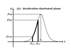
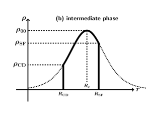
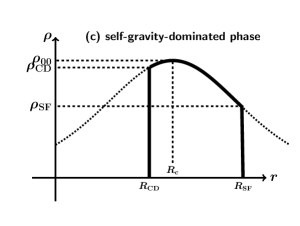
Figure 2.— Schematic pictures of the density profiles of the shell in (a) deceleration-dominated phase $(\Sigma_{\mathrm{s}}<\Sigma_{\mathrm{dec}})$, (b) intermediate phase $(\Sigma_{\mathrm{dec}}<\Sigma_{\mathrm{s}}<2\Sigma_{\mathrm{dec}})$, and (c) self-gravity-dominated phase $(2\Sigma_{\mathrm{dec}}<\Sigma_{\mathrm{s}})$.

Figure 3.— Time evolution of the ratio of the column density $\Sigma_{\mathrm{s}}$ to the characteristic column density $\Sigma_{\mathrm{dec}}$ (Equation (16)). Evolutionary phases corresponding to Figure 2 are labeled.

The time evolution of the density profile is characterized by the ratio of the column density $\Sigma_{\mathrm{s}}$ to the characteristic column density $\Sigma_{\mathrm{dec}}$. Here, the column density $\Sigma_{\mathrm{s}}$ is given by the thin-shell approximation (see Section 2). The column density $\Sigma_{\mathrm{s}}=\rho_{\mathrm{E}}R_{\mathrm{s}}/3$ can be derived from the mass conservation, since $M_{\mathrm{s}}=4\pi GR_{\mathrm{s}}^{2}\Sigma_{\mathrm{s}}$ (see Section 2). The time evolution of the density profile is roughly divided into the following three phases: deceleration-dominated phase ($\Sigma_{\mathrm{s}}<\Sigma_{\mathrm{dec}}$), intermediate phase ($\Sigma_{\mathrm{dec}}<\Sigma_{\mathrm{s}}<2\Sigma_{\mathrm{dec}}$), and self-gravity-dominated phase ($2\Sigma_{\mathrm{dec}}<\Sigma_{\mathrm{s}}$), depending on the value of $\Sigma_{\mathrm{s}}/\Sigma_{\mathrm{dec}}$. The schematic pictures of the density profiles in these three phases are shown in Figures 2. Figure 3 shows the time evolution of $\Sigma_{\mathrm{s}}/\Sigma_{\mathrm{dec}}$. In the early deceleration-dominated phase, $R_{\mathrm{c}}$ is outside of the shell and it is in front of the SF, or $R_{\mathrm{SF}}<R_{\mathrm{c}}$ (see Figure 2(a)). This means that the actual density peak exists at $R_{\mathrm{SF}}$. As the shell expands, $\Sigma_{\mathrm{s}}$ increases by accretion while $\Sigma_{\mathrm{dec}}$ decreases by deceleration. In Figure 3, it is seen that $\Sigma_{\mathrm{s}}$ becomes larger than $\Sigma_{\mathrm{dec}}$ at $t/t_{0}\sim 0.44$. When $\Sigma_{\mathrm{s}}>\Sigma_{\mathrm{dec}}$, $R_{\mathrm{c}}$ is inside the shell. In the intermediate phase ($\Sigma_{\mathrm{dec}}<\Sigma_{\mathrm{s}}<2\Sigma_{\mathrm{dec}}$), $R_{\mathrm{c}}$ is closer to $R_{\mathrm{SF}}$ than $R_{\mathrm{CD}}$ as shown in Figure 2(b). When $\Sigma_{\mathrm{s}}$ becomes larger than $2\Sigma_{\mathrm{dec}}$ ($t/t_{0}>0.57$), $R_{\mathrm{c}}$ becomes closer to $R_{\mathrm{CD}}$ than $R_{\mathrm{SF}}$ (see Figure 2(c)). Since the period of the intermediate phase is relatively short, roughly speaking, the density profile transforms from the deceleration- to the self-gravity-dominated profiles around $t/t_{0}\sim 0.5$.

3.2. Comparison with One-Dimensional Simulation

Obtained density profile by above semi-analytic method is compared with results of 1D simulation. We use the 1D spherically symmetric Lagrangian Godunov method (van Leer, 1997). We do not calculate the radiative transfer of ionizing photons and ionized gas, but the cold gas is pushed by interior pressure whose value is given by Equation (3). The equation of state is assumed to be isothermal. We calculate the expanding shell around the 41$M_{\odot}$ star that is embedded by the uniform ambient gas of $n_{\mathrm{E}}=10^{3}$ cm^-3.

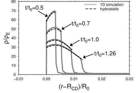
Figure 4.— Snapshots of density profiles for $t/t_{0}=0.5$, 0.7, 1.0, and 1.26. The abscissae are the distance from the CD. The thick gray lines in the upper panel indicate the results of the 1D simulation. The dashed lines in the upper panel represent the instantaneous hydrostatic density profiles.

Figure 4 shows the snapshots of density profiles for $t/t_{0}=0.5$, 0.7, 1.0, and 1.26. The thick gray lines represent the results of the 1D calculation. The dashed lines show the density profiles obtained from the semi-analytic method. It is seen that the semi-analytic method describes the density profile of the 1D simulation reasonably well. The density profile in the semi-analytic method is slightly lower than the results of the 1D calculation because the actual CD expands a little slower than the mean radius of the shell $R_{\mathrm{s}}$ in the thin-shell approximation. As shown in Section 3.1, one can see that the density peak moves the CD from the SF owing to the self-gravity.

3.3. Scaling Law of Unperturbed Density Profiles

As shown in Section 2, the non-dimensional position of the shell, $\tilde{R}_{\mathrm{s}}$, is approximately independent of the model parameters ($n_{\mathrm{E}}$, $Q_{\mathrm{UV}}$). Similarly, it is useful to investigate how the density profile depends on the above parameters. The non-dimensional pressures at the CD and the SF are given by Equation (9) and $\tilde{V}_{\mathrm{s}}^{2}$, respectively, that is, they are independent of the parameters. Moreover, the pressure at the density peak $\tilde{P}_{00}=\tilde{\rho}_{00}\tilde{c}_{\mathrm{s}}^{2}$ is also independent of the parameters as seen in Equation (18). Thus, noting that the non-dimensional sound speed $\tilde{c}_{\mathrm{s}}=c_{\mathrm{s}}t_{0}/R_{0}$ is proportional to the reciprocal of the typical Mach number ${\cal M}_{0}=4R_{0}/(7t_{0}c_{\mathrm{s}})$, where the factor of $4/7$ arises from Equation (4), we have the scaling laws of $\tilde{H_{0}}$, $\tilde{\rho}_{00}$, and $\tilde{t}_{\mathrm{ff}}$ given by

$$\tilde{H}_{0}\propto\tilde{c}^{2}_{\mathrm{s}}\tilde{P}_{00}^{-1/2}\propto{\cal M}_{0}^{-2},$$ (20)

$$\tilde{\rho}_{00}\propto\tilde{c}_{\mathrm{s}}^{-2}\tilde{P}_{00}\propto{\cal M}_{0}^{2},$$ (21)

and

$$\tilde{t}_{\mathrm{ff}}\propto\tilde{\rho}_{00}^{-1/2}\propto\tilde{c}_{\mathrm{s}}\tilde{P}_{00}^{-1/2}\propto{\cal M}_{0}^{-1},$$ (22)

respectively, where $t_{\mathrm{ff}}\equiv 1/\sqrt{2\pi G\rho_{00}}$ is the free fall timescale of the shell. As a result, it is found that the density profiles for various set of $(n_{\mathrm{E}},\;Q_{\mathrm{UV}})$ are characterized by a single parameter, that is the typical Mach number,

$${\cal M}_{0}=\frac{4}{7}\frac{R_{0}}{c_{\mathrm{s}}t_{0}}=7\;Q_{\mathrm{UV,49}}^{1/7}\>T_{\mathrm{c,10}}^{-1/2}\>n_{\mathrm{E,3}}^{-1/14},$$ (23)

where $T_{\mathrm{c,10}}=T_{\mathrm{c}}/10$ K.

4. Influence of Asymmetric Density Profile on Gravitational Instability

As shown in Section 3, the expanding shell has the highly asymmetric density profile and it is expected to influence the GI. In this section, we investigate influences of the asymmetric density profile on the dispersion relation of the GI. What we discuss here is to extend the classical stability analysis of the GI in the symmetric layer with respect to the mid-plane (Goldreich & Lynden-Bell, 1965; Elmegreen & Elmegreen, 1978; Lubow & Pringle, 1993) to the GI in the asymmetric layer. The linear analysis in the incompressible limit has been investigated by Voit (1988).

We take $z$-axis parallel to the thickness of the layer, and take $x$-axis as the transverse direction. The density is assumed to peak at $z=0$, and positions of boundaries are $z_{1}$ and $z_{2}$ ($z_{1}<z_{2}$). We consider a layer that is subject to a constant deceleration. The deceleration arises from the difference of pressures on the boundaries ($z=z_{1}$ and $z_{2}$). In this case, the position of the density peak is not in the mid-plane of the layer, the density profile is asymmetric, or $-z_{1}\neq z_{2}$. The amount of deceleration directly enhances the degree of asymmetry of the density profile.

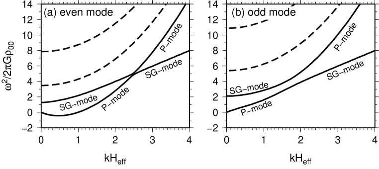
Figure 5.— Dispersion relations for (a) the even mode and (b) the odd mode in the symmetric layer with $|z_{1}|=z_{2}=3H_{0}$. The ordinate denotes $\omega^{2}/2\pi G\rho_{00}$. The abscissa denotes the wavenumber multiplied by the effective thickness of the shell, $H_{\mathrm{eff}}\equiv\sigma/(2\rho_{00})$. The dashed lines show higher harmonics of the sound wave with respect to the $z$-direction.

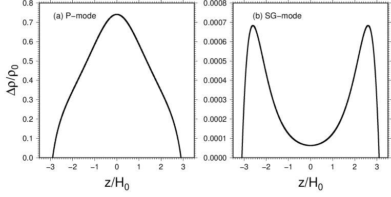
Figure 6.— Distribution of the Lagrangian density perturbation, $\Delta\rho/\rho_{0}\equiv\delta\rho/\rho_{0}+v_{z}\mathrm{d}\ln\rho_{0}(z)\mathrm{d}z$ for $kH_{\mathrm{eff}}=3.5$ in the even mode. Each panel corresponds to (a) the P-mode and (b) the SG-mode. The normalization is determined by $|\delta z_{2}|/z_{2}=0.1$.

4.1. Perturbation Equations

We consider the following perturbations:

$$\rho(z,x,t) = \rho_{0}(z)+\delta\rho(z)e^{i(kx-\omega t)},$$

$$v_{z}(z,x,t) = v_{z}(z)e^{i(kx-\omega t)},$$ (24)

$$v_{x}(z,x,t) = v_{x}(z)e^{i(kx-\omega t)},$$

$$\phi(z,x,t) = \phi_{0}(z)+\delta\phi(z)e^{i(kx-\omega t)}.$$

Perturbation equations are

$$-i\omega\delta\rho+\frac{\mathrm{d}(\rho_{0}v_{z})}{\mathrm{d}z}+\rho_{0}ikv_{x}=0,$$ (25)

$$i\omega v_{z}=\frac{\mathrm{d}}{\mathrm{d}z}\left(c_{\mathrm{s}}^{2}\frac{\delta\rho}{\rho_{0}}+\delta\phi\right),$$ (26)

$$\omega v_{x}=k\left(c_{\mathrm{s}}^{2}\frac{\delta\rho}{\rho_{0}}+\delta\phi\right),$$ (27)

and

$$\frac{\mathrm{d}^{2}\delta\phi}{\mathrm{d}z^{2}}-k^{2}\delta\phi=4\pi G\delta\rho,$$ (28)

where the sound speed is assumed to be constant.

4.1.1 Boundary Conditions

To concentrate on the effect of asymmetry of the unperturbed state, we impose the CD boundary conditions at both $z_{1}$ and $z_{2}$ (Goldreich & Lynden-Bell, 1965; Elmegreen & Elmegreen, 1978) as follows:

$$\delta\rho(z_{1})=-\frac{\mathrm{d}\rho_{0}}{\mathrm{d}z}\Bigr{|}_{z=z_{1}}\delta z_{1},\;\;v_{z}(z_{1})=-i\omega\delta z_{1},$$ (29)

$$\frac{\mathrm{d}\delta\phi}{\mathrm{d}z}\Bigr{|}_{z=z_{1}}-k\delta\phi(z_{1})+4\pi G\rho_{0}(z_{1})\delta z_{1},$$ (30)

and

$$\delta\rho(z_{2})=-\frac{\mathrm{d}\rho_{0}}{\mathrm{d}z}\Bigr{|}_{z=z_{2}}\delta z_{2},\;\;v_{z}(z_{2})=-i\omega\delta z_{1},$$ (31)

$$\frac{\mathrm{d}\delta\phi}{\mathrm{d}z}\Bigr{|}_{z=z_{2}}+k\delta\phi(z_{2})+4\pi G\rho_{0}(z_{2})\delta z_{2},$$ (32)

where $\delta z_{1}$ and $\delta z_{2}$ are the displacements of the surfaces at $z_{1}$ and $z_{2}$, respectively.

4.1.2 Numerical Methods

We solve Equations (25)-(28) as a boundary-value problem for a given wavenumber. Equations (25), (26), and (28) are integrated from $z=z_{1}$ to $z_{2}$ by using the fourth order Runge-Kutta method. Note that $v_{x}$ is determined by $\delta\rho$ and $\delta\phi$ from Equation (27). Given $\omega$, at $z=z_{1}$, we have five unknown variables ($\delta\rho$, $v_{z}$, $\delta\phi$, $\mathrm{d}\delta\phi/\mathrm{d}z$, and $\delta z_{1}$), and have three boundary conditions (see Equations (29) and (30)). Therefore, if we determine two variables $Q_{1}$ and $Q_{2}$, all variables at $z_{1}$ are specified, where $Q_{1}$ is one of ($\delta\rho$, $v_{z}$, $\delta z_{1}$) and $Q_{2}$ is one of ($\delta\phi$, $\mathrm{d}\delta\phi/\mathrm{d}z$). Generally, the boundary conditions at $z_{2}$ are not satisfied if we start from arbitrary values of $Q_{1}$ and $Q_{2}$ at $z_{1}$. Equation (31) can always be satisfied by using a linear combination of two independent solutions having the boundary values $(Q_{1}(z_{1}),\;Q_{2}(z_{1}))=(1,0)$ and (0,1). Eigenvalue, $\omega$, is modified iteratively until the solutions satisfy Equation (32) by using the Newton-Raphson method.

4.2. Symmetric Layer

First, we investigate the symmetric case with $-z_{1}=z_{2}=3H_{0}$. Because of symmetry, perturbation can be divided by even and odd modes completely. In the even (odd) mode, the density perturbation is symmetric (antisymmetric) with respect to the mid-plane. Figures 5(a) and (b) show the dispersion relations for the even and odd modes, respectively. The abscissa denotes the wavenumber multiplied by the effective thickness of the shell, $H_{\mathrm{eff}}\equiv\sigma/(2\rho_{00})$. It is well known that the unstable mode ($\omega^{2}<0$) is found only in the even mode. The unstable mode belongs to the “compressible mode” that means that the density perturbation in the central region collapses leaving behind the gas around boundaries. The detailed structure of stable modes is also plotted in Figure 5. The stable mode can be divided by the “P mode” (pressure mode, or compressible mode) and the “SG mode” (surface-gravity mode). Figure 6 shows that the distribution of the Lagrangian density perturbation $\Delta\rho\equiv\delta\rho+v_{z}\mathrm{d}\rho_{0}/\mathrm{d}z$ for $kH_{\mathrm{eff}}=3.5$ in the even mode. Figures 6(a) and (b) correspond to the P and the SG modes, respectively. The normalization is determined by $|\delta z_{2}|/z_{2}=0.1$. One can see that $\Delta\rho$ profiles of the P and SG modes are quite different. In the P mode, $\Delta\rho/\rho_{0}$ peaks at the mid-plane. The displacement of the boundary $|\delta z_{2}|/z_{2}$ is negligible compared with $\Delta\rho/\rho_{0}$. The P mode propagates as longitudinal variation of pressure. On the other hand, the SG-mode has two $\Delta\rho/\rho_{0}$ peaks near both boundaries, and has the minimum value at the mid-plane. Moreover, since $|\delta z_{2}|/z_{2}$ is much larger than $\delta\rho/\rho_{0}$, the SG mode is almost incompressible. The SG mode propagates as the deformation of the surface. In Figure 5(a), it is seen that the unstable mode transforms into the stable P mode around $kH_{\mathrm{eff}}\sim 1$. On the other hand, there is the another stable mode labelled by the SG mode ($kH_{0}<2$). The P and SG modes approach each other as the wavenumber rises from the small limit. One can see a remarkable feature around $kH_{\mathrm{eff}}\sim 2.5$ where these two modes do not intersect but begin to move apart. At this point, they exchange their properties, suggesting the mode exchange. The mode exchange between the P and the SG modes is also occurred in the odd mode (see Figure 5(b)). This is the first time when the mode exchange is found in the dispersion relation of self-gravitating layer. The dashed lines in Figures 5 show higher harmonics of the sound wave with respect to the $z$-direction. For large wavenumber, the frequencies of the P and the SG modes show different dependence on wavenumber. The P mode shows $k^{2}$ dependence while the SG mode shows $k$ dependence. The angular frequencies of the SG modes associated by the deformation of $z_{1}$ and $z_{2}$ are

$$\omega_{\mathrm{SG,z_{1}}}^{2}=-2\pi G\rho_{0}(z_{1})+\frac{1}{\rho_{0}}\frac{\partial P_{0}}{\partial r}\Bigr{|}_{z_{1}}k$$ (33)

and

$$\omega_{\mathrm{SG,z_{2}}}^{2}=-2\pi G\rho_{0}(z_{2})-\frac{1}{\rho_{0}}\frac{\partial P_{0}}{\partial r}\Bigr{|}_{z_{2}}k,$$ (34)

respectively (Welter & Schmid-Burgk, 1981), for $kH_{0}\gg 1$. The SG branches for large wavenumber in the even and odd modes are identical with each other because the surface gravities at the two boundaries are the same.

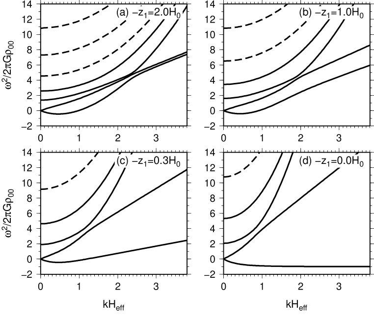
Figure 7.— Dispersion relations for $-z_{1}/H_{0}=$(a)2.0, (b)1.0, (c)0.3, and (d)0.0. The ordinate and the abscissa are the same as Figure 5.

Figure 8.— Cross sections of the layers with the fastest growing mode for (a)$-z_{1}=2.0H_{0}$ and (b)$-z_{1}=0.3H_{0}$. The contour indicates the density perturbation normalized by $\rho_{00}$. The contour levels of the density perturbation take values of 0.04, 0.08, and 0.16.

4.3. Asymmetric Layer

In this section, we investigate the dependence of the dispersion relation on the degree of the asymmetry by changing $z_{1}$. Since the layer is no longer symmetric with respect to $z=0$, perturbations cannot be divided into the even and the odd modes. Figure 7(a) shows the dispersion relation for $z_{1}=-2H_{0}$. One can see more complex structure of the mode exchanges around $kH_{\mathrm{eff}}\sim 2.4$ than that in Figure 5. For large wavenumber, the angular frequencies of the two SG modes split because $\omega_{\mathrm{SG,z_{1}}}^{2}<\omega_{\mathrm{SG,z_{2}}}^{2}$. Figure 8(a) shows the cross section of the layer ($z_{1}=-2H_{0}$) in the fastest growing mode. The contour indicates the density perturbation normalized by $\rho_{00}$. Here, we take $\delta\rho_{\mathrm{max}}/\rho_{00}=0.2$ to specify the normalization of the perturbations. The arrows represent the velocity vectors. The boundary surfaces hardly deform, and the gas collapses from all directions to the center ($z=0$, $x=0$). This behavior corresponds to the compressible mode. In Figure 7(a), the unstable branch transforms the P mode around $kH_{\mathrm{eff}}\sim 1$ and it is connected with the SG mode around $kH_{\mathrm{eff}}\sim 2.4$ through the mode exchange. The case with stronger asymmetry with $z_{1}=-H_{0}$ is shown in Figure 7(b). In this case, the difference of the angular frequencies between the two SG modes is larger because the surface gravity at $z_{1}$ is lower. The frequency of the SG mode associated with $z_{1}$ becomes smaller than that with $z_{2}$. Comparing with Figure 7(a), as well as frequency, the wavenumber of the mode exchange is smaller. As a result, the frequency range of P mode is narrower and the range of the SG mode spreads. The P mode $\omega^{2}\propto k^{2}$ is expected to disappear when the wavenumber of the mode exchange is smaller than a critical wavenumber that separates unstable mode from stable mode.

The case with $-z_{1}<H_{0}$ is quite different from the case with $-z_{1}\geq H_{0}$. The dispersion relation for $-z_{1}=0.3H_{0}$ is shown in Figure 7(c). In Figure 7(c), one can see that the angular frequency of the SG mode $\omega_{\mathrm{SG,z_{1}}}^{2}$ is significantly lower than $\omega_{\mathrm{SG,z_{1}}}^{2}$ for large wavenumbers. Unlike the case with $-z_{1}>H_{0}$, the unstable mode appears to directly connect with the SG mode around $kH_{\mathrm{eff}}\sim 1.2$ as mentioned above. Figure 8(b) shows the cross section of the layer ($z_{1}=-0.3H_{0}$) in the fastest growing mode. The gas tends to collect toward the density peak $z=0$ because the unperturbed gravitational potential has the minimum value there. One can see that eigen-functions in $z>0$ are similar to those in Figure 8(a). The gas collapses toward the center ($z=0$, $x=0$) leaving behind the gas around $z_{2}$. However, in the region where $z<0$, eigenfunctions are quite different. The sound wave can travel between $z_{1}$ and the density peak many times during the development of the GI. Therefore, collapse toward $z=0$ is suppressed by the pressure gradient. However, the GI can proceed even in $z<0$ through the deformation of the $z_{1}$ that makes the gravitational potential deeper. From Figure 8(b), one can see that the velocity field is not headed for the density peak ($z=0)$ but arises so that the surface at $z_{1}$ deforms. Therefore, the features of GI in the region $z>0$ and $z<0$ have properties of “compressible mode” and “incompressible mode”, respectively. If the distance of the $z_{1}$ from the density peak is zero, the layer is unstable for all wavenumbers (see Figure 7(d)).

Figure 9.— Dispersion relation of the asymmetric layer for $-z_{1}/H_{0}=2$(the thick solid line), $1$(the thick dashed line), $0.3$(the thick dotted line), $0.1$(the thin solid line), $0$(the thin dashed line), and $-0.1$(the thin dotted line), where $z_{2}/H_{0}$ is assumed to be $3.0$.

Figure 9 shows the dispersion relation of the unstable mode for variety of $z_{1}$ with $z_{2}=3H_{0}$. The thick solid and the thick dashed lines correspond to $-z_{1}/H_{0}=2$ and 1, respectively. For $-z_{1}/H_{0}\geq 1$, the growth rate $-\omega^{2}/2\pi G\rho_{00}$ decreases as $-z_{1}/H_{0}$ decreases. This property is the same as that in symmetric layers (e.g., see Figure 1 in Nagai et al., 1998). On the other hand, for the cases with $-z_{1}/H_{0}=0.3$ and 0.1, Figure 9 shows that the maximum growth rate increases as $-z_{1}/H_{0}$ decreases, indicating the opposite tendency to the case with $-z_{1}/H_{0}>1$. On the other hand, the wavenumber of the most unstable mode is not different so much. One can see that the square growth rate in large wavenumber is proportional to $\propto k$ while the square growth rate for $-z_{1}/H_{0}>1$ is proportional to $\propto k^{2}$. The unstable mode appears to directly connect with the surface gravity mode at $z_{1}$ whose frequency is given by Equation (33). This is also seen in Figure 10 for $k>k_{\mathrm{max}}$. For $-z_{1}/H_{0}=0$, the surface gravity mode at $z_{1}$ becomes unstable for all wavenumber. In this case, destabilized surface gravity wave has the growth rate $\omega_{\mathrm{SG,z_{1}}}^{2}=-2\pi G\rho(z_{1})<0$ independent of $k$ for large wavenumber limit (see Equation (33)). This is the case with a static shell with $g_{\mathrm{dec}}=0$ (Equation (11)). Tomisaka & Ikeuchi (1983) investigated this situation including shell curvature and found that the shell is unstable for all wavenumber (also see Welter & Schmid-Burgk, 1981). For $-z_{1}/H_{0}=-0.1$, the square growth rate increases as $\propto k$ with wavenumbers because $\omega_{\mathrm{SG,z_{1}}}^{2}\sim\frac{1}{\rho_{0}}\frac{\partial P_{0}}{\partial r}\Bigr{|}_{z_{2}}k<0$ (Equation (11)). This is well-known scaling law of the Rayleigh-Taylor instability. The enhancement of the growth rate for $-z_{1}/H_{0}<1$ arises from the combination of the GI and the Rayleigh-Taylor instability.

5. Gravitational Instability of Expanding Shells

In previous section, we focus on the effect of asymmetry of the density profile by imposing the same boundary conditions in both boundaries. In this section, in a more realistic situation, we investigate the stability of expanding shells driven by the expansion the HII region. The unperturbed density profile at each instant of time is given by the semi-analytic method presented in Section 3. We neglect the curvature effect and solve the perturbation Equations (25)-(28) but $z\rightarrow r$. In this case, as well as in the asymmetric density profile, the difference of boundary properties between leading (the SF) and trailing (the CD) surfaces plays important roles in the GI.

5.1. Influences of Boundaries on the Gravitational Instability

Before presenting a linear analysis, we review how the SF and the CD influence the GI through the boundary effect. This point is important in understanding the results of the linear analysis. In the early phase, the shell is highly confined by the ram pressure on the leading surface and by the thermal pressure on the trailing surface. In this phase, the pressure at boundaries is as large as that at the density maximum, and the thickness of the shell is much smaller than the scale height, $H_{0}=c_{\mathrm{s}}/\sqrt{2\pi G\rho_{00}}$, where $\rho_{00}$ is the maximum density. Thus, in this phase, the boundary effect can strongly influence the GI. In the later phase, the boundary effect of the CD is expected to be also important because the density peak is close to the CD as shown in Section 3.1. In this section, we summarize how the growth rate of GI is controlled by the different boundary conditions. For simplicity, in Section 5.1, the layer is assumed to be symmetric with respect to the mid-plane, and physical variables are averaged across the thickness.

5.1.1 Shock-confined Layer

Many authors have investigated influences of the SF on the GI (Vishniac, 1983; Elmegreen, 1989; Nishi, 1992; Vishniac, 1994; Elmegreen, 1994; Whitworth et al., 1994a; Iwasaki & Tsuribe, 2008). The dispersion relation of the shock-confined layer is given by

$$\omega^{2}\simeq c_{\mathrm{s}}^{2}k^{2}-2\pi Gk\Sigma_{\mathrm{s}},$$ (35)

where $\Sigma_{\mathrm{s}}$ is the column density, and $k$ is the transverse wavenumber of the perturbation. This dispersion relation is the same as that for the infinitesimally thin layer. In the highly confined layer, it is well known that the perturbation behaves like incompressible mode because the sound-crossing time over the thickness is much smaller than the free-fall timescale, $\sim 1/\sqrt{G\rho_{00}}$ (Elmegreen & Elmegreen, 1978; Lubow & Pringle, 1993). Therefore, density fluctuation is small. The layer becomes unstable mainly by the deformation of the surfaces that makes the perturbation of the gravitational potential deeper. Hereafter, we call this mode the “incompressible mode”. The deformation of the SF generates the tangential flow carrying the gas from the convex to the concave regions (seen from the downstream). Therefore, the tangential flow tends to make the SF flat, suggesting that it suppresses the growth of the GI. In the shock-confined layer, the restoring term $c_{\mathrm{s}}^{2}k^{2}$ arises from the tangential flow behind the oblique SF. On the other hand, in the case of the infinitesimally thin layer, this term comes from the pressure gradient. Therefore, the origin of the restoring force is quite different. From Equation (35), the maximum growth rate is given by $\pi G\Sigma_{\mathrm{s}}/c_{\mathrm{s}}$, and the corresponding wavenumber is given by $\pi G\Sigma_{\mathrm{s}}/c_{\mathrm{s}}^{2}$. When $\Sigma_{\mathrm{s}}$ is small ($\leq\rho_{00}H_{0})$, the maximum growth rate is smaller than the inverse of the free-fall timescale, $\sqrt{G\rho_{00}}$, and the corresponding scale is larger than the scale height $H_{0}$ that is comparable to the Jeans scale.

5.1.2 Pressure-confined Layer

Next, we review the influence of the CD on the GI. We consider the layer confined by thermal pressure of hot rarefied gases (CD boundary condition) on both sides. The dispersion relation becomes

$$\omega^{2}\simeq 2\pi G\Sigma_{\mathrm{s}}L_{\mathrm{s}}k^{2}-2\pi Gk\Sigma_{\mathrm{s}},$$ (36)

where $L_{\mathrm{s}}$ is the thickness of the layer, and we consider the large-scale limit where $k\ll 1/L_{\mathrm{s}}$. Detailed derivation of Equation (36) is shown in Appendix 3 of Iwasaki & Tsuribe (2008). In the pressure-confined layer, the stabilization effect of the tangential flow does not exist. Therefore, the restoring term in Equation (36) is quite different from that in Equation (35). Using the gravitational acceleration at the surfaces as $|g|=2\pi G\Sigma_{\mathrm{s}}$, we can express the restoring term in Equation (36) by $|g|L_{\mathrm{s}}k^{2}$. Therefore, one can see that the restoring force arises from the surface gravity wave. The layer with the CD boundary condition is less stabilized compared with the shock boundary condition because the phase velocity of the gravity wave $\sqrt{|g|L_{\mathrm{s}}}$ is much smaller than $c_{\mathrm{s}}$ when $L_{\mathrm{s}}\ll H_{0}$. From the dispersion relation (36), the maximum growth rate is comparable to the inverse of the free fall time of the layer $\simeq\sqrt{G\rho_{00}}$, and the corresponding wavelength is about the thickness of the layer, $\simeq L_{\mathrm{s}}$ (Elmegreen & Elmegreen, 1978; Lubow & Pringle, 1993). Therefore, one can see that the most unstable mode in the pressure-confined layer has a larger growth rate and a smaller scale than the shock-confined layer (see Figure 9 of Iwasaki & Tsuribe, 2008, in detail).

5.1.3 Expanding Shells

Equations (35) and (36) cannot be applied directly in the GI of the expanding shells because the GI is expected to be stabilized by evolutionary effects, such as the expansion of the shell and the accretion of fresh gas through the SF. Elmegreen (1994) derived the following approximate dispersion relation,

$$i\omega=-\frac{3V_{\mathrm{s}}}{R_{\mathrm{s}}}+\sqrt{\left(\frac{V_{\mathrm{s}}}{R_{\mathrm{s}}}\right)^{2}+2\pi Gk\Sigma_{\mathrm{s}}-c_{\mathrm{s}}^{2}k^{2}}.$$ (37)

The terms with $V_{\mathrm{s}}/R_{\mathrm{s}}$ come from evolutionary effects that stabilize the GI.

One can see that Equation (37) for the limit of $V_{\mathrm{s}}/R_{\mathrm{s}}\rightarrow 0$ is the same as Equation (35). Therefore, Elmegreen (1994) and Whitworth et al. (1994b) essentially applied Equation (35) in the context of the GI of the expanding shell. However, they did not take into account the boundary effect of the CD on the trailing surface. Comparing Equations (35) and (36), we suggest that the stability of the thin shell neglecting the effect of the CD is suffered by large stabilizing effect, and it will underestimate the growth rate of GI in expanding shells.

5.2. Boundary Condition

First, we assume that a constant pressure exerts on the CD all the time (the CD boundary condition; Goldreich & Lynden-Bell, 1965; Elmegreen & Elmegreen, 1978). The boundary conditions are

$$\delta\rho(R_{\mathrm{CD}})=-\frac{\mathrm{d}\rho}{\mathrm{d}r}\Bigr{|}_{r=R_{\mathrm{CD}}}\delta R_{\mathrm{CD}},\;\;\;v_{r}(R_{\mathrm{CD}})=i\omega\delta R_{\mathrm{CD}},$$ (38)

and

$$\frac{\mathrm{d}\delta\phi}{\mathrm{d}r}-k\delta\phi+4\pi G\rho(R_{\mathrm{CD}})\delta R_{\mathrm{CD}}=0,$$ (39)

where $\delta R_{\mathrm{CD}}$ is the displacement of the CD.

Next, let us consider the boundary conditions at $r=R_{\mathrm{SF}}$. Since the unperturbed state is assumed to be the hydrostatic configuration, it is impossible to impose the shock boundary conditions self-consistently. In order to treat it self-consistently, time-dependent initial value problem is needed to be solved (Welter, 1982; Iwasaki & Tsuribe, 2008). Therefore, in this paper, we mimic the shock boundary conditions by introducing the stabilization effect. We consider the following two approximate boundary conditions.

Rigid surface boundary condition (RSBC). $\frac{\;\;\;\;\;\;}{\;\;\;\;\;\;}$ Voit (1988) and Usami, Hanawa & Fujimoto (1995) assumed that no ripples arise on the surface, or $\delta R_{\mathrm{SF}}=0$, where $\delta R_{\mathrm{SF}}$ is the displacement of the SF. The reason why we adopt $\delta R_{\mathrm{SF}}=0$ is that the thin-shell linear analysis of the layer confined by rigid surfaces gives the same dispersion relation as that of the shock-confined layer (Equation (35)). In more precisely, in the shock-confined layer, the tangential flow boosts the suppression effect against the self-gravity as mentioned in Section 5.1.1. Instead, the RSBC weakens the self-gravity.

Tangential flow boundary condition (TSBC). $\frac{\;\;\;\;\;}{\;\;\;\;\;}$ If the SF is rippled, the tangential flow behind the SF is generated. Therefore, we set the tangential velocity $v_{x}$ at $r=R_{\mathrm{SF}}$. Linearizing the Rankine-Hugoniot relation, we have

$$v_{x}(R_{\mathrm{SF}})=-\left(\dot{R}_{\mathrm{SF}}-\frac{c_{\mathrm{s}}^{2}}{\dot{R}_{\mathrm{SF}}}\right)ik\delta R_{\mathrm{SF}}.$$ (40)

The detailed derivation of Equation (40) is found in Iwasaki & Tsuribe (2008).

With both of above boundary conditions (RSBC and TFBC), we also impose the following ordinary used boundary conditions,

$$v_{r}(R_{\mathrm{SF}})=i\omega\delta R_{\mathrm{SF}},$$ (41)

and

$$\frac{\mathrm{d}\delta\phi}{\mathrm{d}r}+k\delta\phi+4\pi G\rho(R_{\mathrm{SF}})\delta R_{\mathrm{SF}}=0.$$ (42)

It is well known that the SF of the deceleration shell is subject to the hydrodynamical overstability (Vishniac, 1983). The linear analysis in this paper cannot capture the Vishniac instability (VI) correctly since the approximate shock boundary conditions are imposed. The effect of the VI is discussed in Section 6.

The numerical method is the same as that in Section 4.1.2.

5.3. Scaling Law of Dispersion Relations

As shown in Section 3.3, it is found that the density profiles are characterized by a single parameter ${\cal M}_{0}$. This is because the scale height, the peak density, and the free fall time have the scaling laws with respect to ${\cal M}_{0}$ as shown in Equations (20)-(22). The same is the case with the perturbation equations and the dispersion relation. The non-dimensional maximum growth rate $\tilde{\omega}_{\mathrm{max}}\equiv\omega_{\mathrm{max}}t_{0}$ and the corresponding wavenumber $\tilde{k}_{\mathrm{max}}\equiv k_{\mathrm{max}}R_{0}$ scale as $\propto{\cal M}_{0}$ and $\propto{\cal M}_{0}^{2}$, respectively. Therefore, in the present model, the evolution of the shell for various set of $(n_{\mathrm{E}},\>Q_{\mathrm{UV}})$ can be described by a single unperturbed profile and a single time-dependent dispersion relation that are normalized by $H_{0}$, $\rho_{00}$, and $t_{\mathrm{ff}}$. The result can be applicable to a wide range of parameters simply by using the scaling relation on ${\cal M}_{0}$.

5.4. Results

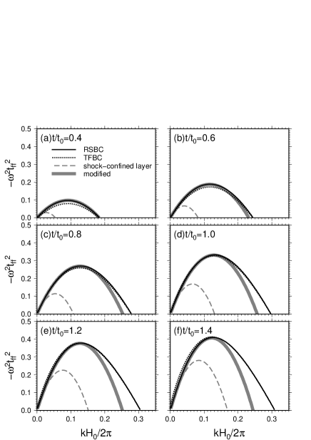
Figure 10.— Dispersion relations derived from our linear analysis using RSBC (the solid lines) and TFBC (the dotted lines). For comparison, the dispersion relation of shock-confined layer (Equation (35)) is plotted by the dashed gray lines. The thick gray lines represent modified dispersion relation (Equation (43)). The abscissa and ordinate axes indicate the wavenumber $kH_{0}/2\pi$ and the growth rate normalized by $t_{\mathrm{ff}}=1/\sqrt{2\pi G\rho_{00}}$, respectively.

Figure 11.— Time evolution of the ratio of $c_{\mathrm{eff}}$ to $c_{\mathrm{s}}$.

Figure 12.— Cross section of the shell is plotted using eigenfunctions. The corresponding time and angular wavenumber are $t/t_{0}=1.3$ and $l=52$, respectively. The contour indicates the density perturbation normalized by $\rho_{00}$. The vectors represent velocity perturbations.

At any time, the unperturbed state is given by the procedure in Section 3. Perturbation Equations (25)-(28) are solved as the eigenvalue- and boundary-value problem. As a result, the growth rate, $\omega(k,t)$ can be obtained as a function of the wavenumber and time.

First, we present the results of the linear analysis in Figure 10 at various epochs. The ordinate and the abscissa axes represent the non-dimensional growth rate $\omega t_{\mathrm{ff}}$ and wavenumber $kH_{0}/2\pi$. The solid and the dotted lines indicate the results of the linear analysis using RSBC and TFBC, respectively. We refer the growth rates obtained by using RSBC and TFBC to $\omega_{\mathrm{RSBC}}$ and $\omega_{\mathrm{TFBC}}$, respectively. The dependence of the dispersion relation on the parameters $(n_{\mathrm{E}},\>Q_{\mathrm{UV}})$ can be eliminated by using non-dimensional growth rate $\omega t_{\mathrm{ff}}$ and wavenumber $kH_{0}$ as shown in Section 5.3. We have confirmed that the dispersion relation is identical to that with other parameter sets of $(n_{\mathrm{E}},\;Q_{\mathrm{UV}})$ by using the non-dimensional quantities. Figure 10 shows that the difference between $\omega_{\mathrm{RSBC}}$ and $\omega_{\mathrm{TFBC}}$ is negligible although RSBC and TFBC are physically quite different.

In this analysis, we do not take into account the evolutionary effects, such as the expansion and accretion of the gas. Therefore, we compare the results of the linear analysis with the dispersion relation of the shock-confined layer (Equation (35)) rather than that of the expanding shell (Equation (37)). One can see that the growth rate is larger than the prediction from the shock-confined layer. As shown in Section 5.1, this difference comes from the boundary effect of the CD. Therefore, the shell is expected to begin to grow earlier and to fragment more quickly than the prediction from Elmegreen (1994) that is based on Equation (35).

The dispersion relation with CD + SF boundary conditions is expected to lie between that with SF + SF (Equation (35)) and that with CD + CD (Equation (36)). Therefore, to approximate the dispersion relation with RSBC analytically, we combine Equation (35) with Equation (36) as follows:

$$\omega_{\mathrm{mod}}^{2}=c_{\mathrm{eff}}^{2}k^{2}-2\pi Gk\Sigma_{\mathrm{s}},$$ (43)

where $c_{\mathrm{eff}}$ is the effective sound speed,

$$c_{\mathrm{eff}}=\sqrt{A2\pi G\Sigma_{\mathrm{s}}L_{\mathrm{eff}}+\left(\frac{c_{\mathrm{s}}}{2}\right)^{2}},$$ (44)

where $A$ is a parameter and $L_{\mathrm{eff}}=\Sigma_{\mathrm{s}}/\rho_{00}$ is the effective thickness that approaches the actual thickness $L_{\mathrm{s}}$ for small $\Sigma_{\mathrm{s}}$ and $2H_{0}$ for large $\Sigma_{\mathrm{s}}$. The first and the second terms inside the square root correspond to the effect of the CD and the SF boundary conditions, respectively. Here, we choose the parameter $A$ by the condition where the maximum value of $\omega_{\mathrm{mod}}$ coincides with that of $\omega_{\mathrm{RSBC}}$. As a result, it is found that a single value of $A=0.39$ shows good agreement in growth rates between the modified dispersion relation and the detailed linear analysis. The modified dispersion relations in Equation (43) are plotted by the thick gray lines in Figure 10. In Figure 10, one can see that $\omega_{\mathrm{mod}}$ well describes $\omega_{\mathrm{RSBC}}$ for $k<k_{\mathrm{max}}$ all the time. This suggests that simply Equation (43) can describe the most unstable mode obtained by the detailed linear analysis all the time. Figure 11 shows the time evolution of the effective sound speed. In the early phase, $c_{\mathrm{eff}}$ is about $0.5c_{\mathrm{s}}$, suggesting that the effect of the CD diminishes the effective sound speed $c_{\mathrm{eff}}$ by half in Equation (35). As the shell expands, $c_{\mathrm{eff}}$ increases.

The effect of asymmetric density is seen in Figure 10 where it is found that $\omega_{\mathrm{mod}}$ deviates from $\omega_{\mathrm{RSBC}}$ for $k>k_{\mathrm{max}}$ in the gravity-dominated phase ($t/t_{0}>0.5$). This is because $\omega_{\mathrm{mod}}^{2}$ connects with the P mode $\propto k^{2}$ while $\omega_{\mathrm{RSBC}}^{2}$ connects with the SG mode $\propto k$ as shown in Section 4.

The predicted cross section of the shell by the linear analysis for $(Q_{\mathrm{UV}}=10^{48.78}$ $\mathrm{s^{-1}}$, $n_{\mathrm{E}}=10^{3}$ $\mathrm{cm}^{-3})$ is shown in Figure 12 by using the eigenfunctions. The corresponding time is $t/t_{0}=1.3$ and the angular wavenumber is $l=52$. In Figure 12, the gas tends to accumulate onto the peak only through the upper half region $r>R_{\mathrm{c}}$. This property of the flow can be seen from the direction of arrows in Figure 12. Actually, in the upper half region, we find $R_{\mathrm{SF}}-R_{\mathrm{c}}=1.05H_{0}>H_{0}$ that represents that the gas can collapse to the peak because the sound wave cannot travel from $R_{\mathrm{c}}$ to $R_{\mathrm{SF}}$ within the free fall time. On the other hand, in the region of bottom half ($r<R_{\mathrm{c}}$), we find that $R_{\mathrm{c}}-R_{\mathrm{CD}}=0.285H_{0}<H_{0}$. This indicates that the gas in $r<R_{\mathrm{c}}$ cannot collapse to the peak because the sound wave can travel from $R_{\mathrm{c}}$ to $R_{\mathrm{CD}}$ many times within the free fall time. Thus, the pressure gradient prevents the compression of gas in the region $r<R_{\mathrm{c}}$. However, the GI can proceed even in $r<R_{\mathrm{c}}$ through the deformation of the CD that makes the gravitational potential deeper. Therefore, the features of GI in the region $r>R_{\mathrm{c}}$ and $r<R_{\mathrm{c}}$ have the properties of the “compressible mode” and “incompressible mode”, respectively.

6. Discussion

The gravitational fragmentation of expanding shells confined from both sides by the CD was investigated by Dale et al. (2009) numerically and by Wünsch et al. (2010) using analytical approximations. They assumed that the thermal pressure on both sides is the same and temporally constant. Therefore, the density peak is always around the mid-plane of the shell, and the density profile is almost symmetric. In their calculation, the column density decreases with time because the shell expands keeping the mass fixed. Therefore, the pressures at the boundaries approach to the peak pressure. They found that the confining pressure accelerates fragmentation in the later phase, and described this effect as “pressure-assisted” gravitational fragmentation. This mode is the same as the incompressible mode in this paper. Wünsch et al. (2010) established a semi-analytic linear analysis that explains results of Dale et al. (2009).

The linear analysis in this paper cannot describe the VI correctly since the approximate shock boundary conditions are imposed in Section 5. The original analysis by Vishniac (1983) did not find the finite scale most unstable mode because the thickness of the shell is neglected. Vishniac & Ryu (1989) derived a simple analytic dispersion relation of the VI for a decelerating isothermal spherical shock wave taking into account the effect of the thickness (also see Ryu & Vishniac, 1987). Although, their analysis did not include the self-gravity, here, we use their dispersion relation (see Equations 19(a) and (b) in their paper) to estimate the effect of the VI. Their dispersion relation depends on the Mach number ${\cal M}$ of the shell and the expansion law. For the case with the expanding HII regions, the shell expands as $\propto t^{4/7}$ if the self-gravity is neglected. In this case, the perturbation grows not exponentially but in a power-law $\propto t^{s}$, where $s$ characterizes the growth rate. Figure 13 shows the real part of $s$ as a function of the angular wavenumber $l$. One can see that the maximum growth rate $\mathrm{Re}(s)$ increases with ${\cal M}$. The angular scale of the most unstable mode is smaller for larger $\cal M$. We find that the unstable mode exists only for ${\cal M}\geq 4.7$. To see the typical value of the Mach number, we consider the expanding shell around the 41$M_{\odot}$ star that is embedded by the uniform ambient gas of $n_{\mathrm{E}}=10^{3}$ cm^-3. Figure 14 shows the Mach number of the shell for $T_{\mathrm{c}}$ = 10 K (the solid line) and 30 K (the dashed line). In the early phase when the self-gravity is not important ($t/t_{0}<0.5$), since the Mach number is as large as several tens, Re$(s)$ is large. The small scale perturbation with $l=10^{2}\sim 10^{3}$ quickly grows and saturates in the nonlinear stage (Mac Low & Norman, 1993). On the other hand, in the later phase (the self-gravity-dominated phase, $t/t_{0}>0.5$), the Mach number is as low as $5-10$ as shown in Figure 14. In this phase, Re$(s)\sim 1$ from Figure 13. This means that the growth rate of the perturbations is comparable to the expansion rate $\propto t^{4/7}$. Therefore, in the self-gravity-dominated phase, the VI is not expected to be important. The influence of VI on the GI is expected to be only the increase of the initial amplitude of perturbations for the GI.

Figure 13.— Growth rate of the VI when the shell expands as $\propto t^{4/7}$. Each line corresponds to ${\cal M}=4.7$, 10, 7, and 4.7.

Figure 14.— The Mach number of the shell for $Q_{\mathrm{UV}}=10^{49}\>s^{\mathrm{-1}}$ and $n_{\mathrm{E}}=10^{3}$ cm^-3. The solid and the dashed lines indicate the case with $T_{\mathrm{c}}$=10 K and 30 K, respectively.

7. Summary

In this paper, we have performed linear perturbation analysis of decelerating shells created by the expansion of HII regions. We summarize our results as follows:

1. We develop a semi-analytic method for describing the density profile in the shell. The time evolution of the density profile of the expanding shell can be divided into three phases, deceleration-dominated, intermediate, and self-gravity-dominated phase. In the deceleration-dominated phase, the density peak is in SF by the inertia force owing to the deceleration. As the shell mass increases and the self-gravity becomes important, the density peak is inside the shell, but it is closer to the SF than the CD in the intermediate phase. In the self-gravity-dominated phase, the shell becomes massive and the density peak is closer to the CD than the SF. The evolution is confirmed by 1D hydrodynamical simulation.

2. We show detailed structures of dispersion relation in the asymmetric layer subjected to a constant deceleration both of unstable and stable modes by imposing the CD boundary condition from/at both sides.

   • We discover the mode exchange between the compressible and surface-gravity modes in the stable regime.

   • In a situation where the distance from one surface $z_{1}$ to the density peak $z=0$ is smaller than the scale height of the self-gravity $H_{0}$ and the distance from the other surface $z_{2}$ to $z=0$ larger than $H_{0}$, the nature of the GI is quite different from the symmetric case with the same column density and the peak density. The eigenfunction in the region $0<z<z_{2}$ is approximately the compressible mode. On the other hand, the eigenfunction in the region $z_{1}<z<0$ is approximately the incompressible mode. Moreover, the growth rate is enhanced compared with symmetric cases through cooperation with the Rayleigh-Taylor instability.

3. We investigate linear stability of expanding shells driven by HII regions taking into account the shock-like boundary condition on the leading surface, the CD boundary condition on the trailing surface, and the asymmetric density profile obtained by the semi-analytic method.

   • The shell is expected to grow earlier than the prediction of previous studies (Elmegreen, 1994; Whitworth et al., 1994b) that are based on the dispersion relation of the shock-confined layer.

   • In the self-gravity-dominated phase, since the density peak is closer to the CD than the SF, the CD is expected to deform significantly.

These results provide useful knowledge for the analysis of more detailed nonlinear numerical simulations that is the scope of our next paper (Iwasaki et al., 2011).

References

- Dale et al. (2007) Dale, J. E., Bonnell, I. A. & Whitworth, A. P. 2007, MNRAS, 375, 1291
- Dale et al. (2009) Dale, J. E., Wünsch, R., Whitworth, A. P., & Palouš, J. 2009, MNRAS, 398, 1537
- Deharveng et al. (2010) Deharveng, L., et al. 2010, A&A, 523, A6
- Elmegreen & Elmegreen (1978) Elmegreen, B. G., & Elmegreen, D. M. 1978, ApJ, 220, 1051
- Elmegreen (1994) Elmegreen, B. G. 1994, ApJ, 427, 384
- Elmegreen (1989) Elmegreen, B. G. 1989, ApJ, 340, 786
- Elmegreen & Lada (1977) Elmegreen, B. G., & Lada, C. J. 1977, ApJ, 214, 725
- Goldreich & Lynden-Bell (1965) Goldreich, P., & Lynden-Bell, D. 1965, MNRAS, 130, 7