Numerical Hermitian Yang-Mills Connections
and Kähler Cone Substructure

Lara B. Anderson¹, Volker Braun², and Burt A. Ovrut¹

¹Department of Physics, University of Pennsylvania¹
209 South 33rd Street, Philadelphia, PA 19104-6395, U.S.A.
²Dublin Institute for Advanced Studies²
10 Burlington Road, Dublin 4, Ireland.

We further develop the numerical algorithm for computing the gauge connection of slope-stable holomorphic vector bundles on Calabi-Yau manifolds. In particular, recent work on the generalized Donaldson algorithm is extended to bundles with Kähler cone substructure on manifolds with $h^{1,1}>1$. Since the computation depends only on a one-dimensional ray in the Kähler moduli space, it can probe slope-stability regardless of the size of $h^{1,1}$. Suitably normalized error measures are introduced to quantitatively compare results for different directions in Kähler moduli space. A significantly improved numerical integration procedure based on adaptive refinements is described and implemented. Finally, an efficient numerical check is proposed for determining whether or not a vector bundle is slope-stable without computing its full connection.

Email: andlara@physics.upenn.edu, vbraun@stp.dias.ie, ovrut@elcapitan.hep.upenn.edu

1 Introduction

In this paper, we explore $\mathcal{N}=1$ supersymmetric vacua of $E_{8}\times E_{8}$ heterotic string [1, 2] and $M$-theory [3, 4, 5, 6, 7, 8]. The four-dimensional effective theory is specified by a Calabi-Yau threefold $X$ and a slope-stable holomorphic vector bundle, $\mathscr{V}$. The detailed structure of the low energy theory is determined [9] by the choice of a Ricci-flat metric, $g$, on the threefold and an $\mathcal{N}=1$ supersymmetry gauge connection, $A$, on the vector bundle. Existence proofs, such as Yau’s theorem [10] for the Ricci-flat metric and the Donaldson-Uhlenbeck-Yau theorem [11, 12] for the Hermitian Yang-Mills connection, provide us with numerous examples of such geometries. However, the explicit metric and gauge connection are not known analytically, except in very special cases [13, 14, 15, 16, 17, 18]. The difficulty of determining these quantities has presented an obstacle to the systematic search for realistic heterotic vacua. Even for a known vacuum, this has precluded the computation of physically relevant parameters in the effective theory, such as the Yukawa couplings.

In recent years, the development of sophisticated numerical approximation schemes have provided a new approach to these problems [19, 20, 21, 22, 23, 24, 25, 26, 27, 28]. With the development of powerful new algorithms and modern computer speed, it is now possible to numerically approximate Ricci-flat metrics and Hermitian Yang-Mills connections to a high degree of accuracy. We will refer to these tools collectively as the “generalized Donaldson algorithm”. Using them, the structure of the four-dimensional effective theory can be explored in remarkable new ways. The goal of this program is to determine all coefficients in the superpotential, the explicit form of the Kähler potential and, ultimately, to perform first-principle calculations of physical quantities such as the relative quark and lepton masses.

In this paper, we make substantial progress towards this goal by extending previous work [29] to include vector bundles defined over manifolds with higher-dimensional Kähler cones; that is, for which $h^{1,1}>1$. Importantly, our results allow one to study arbitrary vector bundles arising in heterotic string compactifications and to determine whether such geometries admit $\mathcal{N}=1$ supersymmetric vacua. The problem of finding the Kähler cone substructure, that is, the regions in Kähler moduli space where a given holomorphic vector bundle is or is not slope-stable, is a notoriously difficult one. In particular, the difficulty of a direct stability analysis generally increases rapidly with the dimension $h^{1,1}$ of the Kähler cone. One of the great advantages of the algorithm presented in this paper is that, unlike a standard analytic analysis, our numerical calculations can be performed with essentially equal ease in arbitrary $h^{1,1}$. This provides an important new tool in the study of supersymmetric heterotic vacua.

The structure of the paper is as follows. To begin, in Section 2 we provide a brief review of the numerical algorithm for computing the Ricci-flat metric, $g$, and the Hermitian Yang-Mills connection, $A$. Starting in Section 3, an overview of Donaldson’s algorithm for computing the Ricci flat metric [19, 20, 21] on a Calabi-Yau manifold is given. In particular, the numerical implementations developed in [30, 31] and [32, 24] are discussed. Next, in Subsection 3.2, we outline the recent generalizations of Donaldson’s algorithm presented in [23, 24, 29]. These make it possible to compute Hermite-Einstein metrics on holomorphic vector bundles over a Calabi-Yau manifold and, hence, to solve for the unique gauge connection satisfying the conditions for $\mathcal{N}=1$ supersymmetry.

Both the original Donaldson algorithm and its generalizations to connections rest on finding a particularly “nice” projective embedding. In the case of the Ricci-flat metric on a Calabi-Yau manifold, the embedding is defined from $X$ into some higher-dimensional projective space via the global sections of some ample line bundle, ${\cal L}^{\otimes k_{g}}$, on $X$. In the case of the connection on a rank $n$ bundle $\mathscr{V}$, a map into the Grassmannian $G(n,N_{k_{H}}-1)$ is constructed out of the $N_{k_{H}}$ sections of $\mathscr{V}\otimes{\cal L}^{\otimes k_{H}}$, where ${\cal L}^{\otimes k_{H}}$ is some ample line bundle on $X$. Using either one of these embeddings, a metric can be pulled-back to the Calabi-Yau manifold and vector bundle, respectively. One obtains a $k_{g}$-dependent sequence of Kähler metrics $X$ and a $k_{H}$-dependent sequence of Hermitian fiber metrics on $\mathscr{V}$. The degrees of freedom of every embedding parametrize a family of pulled-back metrics. By tuning the embedding to the so-called “balanced embedding” for each degree $k_{g}$ and $k_{H}$, the Kähler metrics converge to the Ricci-flat metric on $X$ and the Hermitian fiber metrics converge to a Hermite-Einstein metric on $\mathscr{V}$. Finding the balanced embedding is solved by Donaldson’s T-operator and its generalization due to Wang and others [19, 33, 20, 21, 22, 23, 34, 35]. Roughly, the T-operator acts on embeddings of fixed degree and has the balanced embedding as a fixed point. For a Calabi-Yau manifold, iterating the T-operator will always converge to a balanced embedding, and, therefore, to the Ricci-flat metric on $X$ in the limit that $k_{g}\to\infty$. In the case of the connection, the iteration of the T-operator for fixed $k_{H}$ is not guaranteed to converge. In fact, it converges to a balanced embedding if and only if the bundle $\mathscr{V}$ is Gieseker-stable. Furthermore, when $\mathscr{V}$ is slope-stable then the sequence of balanced embeddings define a fiber metric converging to the Hermite-Einstein fiber metric in the limit that $k_{H}\to\infty$.

In Section 4, we modify a number of the numerical tools developed in previous work [29] to enable us to compare the convergence of the generalized Donaldson algorithm for different rays (or “polarizations”) in Kähler moduli space. These results are illustrated in Subsection 4.2 by an indecomposable, rank $2$ vector bundle defined over the $K3$ surface via the monad construction [36, 37, 38]. Furthermore, in Section 5, we present the technical details of a newly developed, rapid numerical scheme for integrating over a Calabi-Yau manifold.

Section 6 provides a criterion to decide whether or not a vector bundle is slope-stable for a given polarization, without the need to explicitly compute the connection. Hence, this check can be rapidly applied to decide slope stability. In particular, we use a result of Wang [23] which states that the iteration of the T-operator will reach a fixed point if and only if the defining vector bundle is Gieseker-stable. While Gieseker stability is not sufficient to guarantee a solution to the Hermitian Yang-Mills equations (and, hence, a supersymmetric heterotic vacuum), it still provides valuable information. In particular, while a slope-stable bundle is automatically Gieseker stable, the converse does not follow. A Gieseker-stable bundle need only be slope semi-stable. Despite these subtleties, we extract results from the T-operator convergence which can be used to determine the Kähler cone substructure. Related to the question of semi-stability, we consider the dependence of slope-stability on the vector bundle moduli $H^{1}(\mathscr{V}\otimes\mathscr{V}^{\vee})$ in Section 7. In particular, the numerical algorithm is tested on a “stability wall” [39, 40] in Kähler moduli space, the boundary between slope-stable and unstable regions. We find that the generalized Donaldson algorithm is sensitive to the bundle moduli dependence and, hence, our results also distinguish the marginal cases of slope poly-stable bundles from strictly semi-stable ones.

In Section 8, we extend our study to higher-dimensional spaces by presenting an example of Kähler cone substructure of a rank $3$ monad bundle defined over a Calabi-Yau threefold constructed as a complete intersection in a product of projective spaces. We conclude and discuss future work in Section 9.

2 Hermitian Yang-Mills Connections and Fiber Metrics

A supersymmetric $E_{8}\times E_{8}$ heterotic string compactification is specified by 1) a complex $d$-dimensional Calabi-Yau manifold, $X$, and 2) a holomorphic vector bundle, $\mathscr{V}$, with structure group $K\subset E_{8}$ defined over $X$. The gauge connection, $A$, on $\mathscr{V}$ with associated field strength, $F$, must satisfy the well-known Hermitian Yang-Mills (HYM) equations [9]. For general $U(n)$ structure groups, these equations are given by

$$F_{ij}=F_{\bar{i}\bar{j}}=0,\qquad g^{i\bar{j}}F_{i\bar{j}}=\mu(\mathscr{V})\cdot\mathbf{1}_{n\times n},$$ (2.1)

where $g^{i\bar{j}}$ is the Calabi-Yau metric, $n$ is the rank of $\mathscr{V}$, the scalar $\mu(\mathscr{V})$ is a real number associated with $\mathscr{V}$ and $i,j=1,\ldots d$, run over the holomorphic indices of the Calabi-Yau $d$-fold. Our primary interest is in Calabi-Yau threefolds, since compactification on these give rise to $\mathcal{N}=1$ supersymmetric theories in four dimensions. However, in order to present simple illustrations of the techniques introduced in this paper, we will discuss Calabi-Yau twofold ($K3$) as well as threefold examples. It is not strictly necessary for the first Chern class of the bundle to vanish [41], and the methods used in this paper would work just as well in that setting. However, most realistic compactifications are based on structure groups $K=SU(n)\subset U(n)$, and these will be our main focus. When $K=SU(n)$, the parameter $\mu(\mathscr{V})=0$ and eq. (2.1) reduces to

$$F_{ij}=F_{\bar{i}\bar{j}}=0,\qquad g^{i\bar{j}}F_{i\bar{j}}=0.$$ (2.2)

While eq. (2.2) are the relevant equations for realistic heterotic compactifications, mathematically it will often be useful to discuss the Hermitian Yang-Mills equations in full generality.

A solution to (2.1) is equivalent to the bundle $\mathscr{V}$ carrying a particular Hermitian structure. An Hermitian structure (or Hermitian fiber metric), $G$, on $\mathscr{V}$ is an Hermitian scalar product $G_{x}$ on each fiber $\mathscr{V}(x)$ which depends differentiably on $x$. The pair $(\mathscr{V},G)$ is often referred to as an Hermitian vector bundle. For a given frame, $e_{a}(x)$, the Hermitian structure specifies an inner product as

$$(e_{a},e_{b})=G_{{\bar{a}}b},\qquad G=G^{\dagger}.$$ (2.3)

A choice of frame provides the necessary coordinates to express the covariant derivative in terms of the connection,

$$D(v^{a}e_{a})=(dv^{a})e_{a}+v^{a}A^{b}_{a}e_{b}.$$ (2.4)

Imposing compatibility of the connection with the holomorphic structure of the bundle and the fiber metric determines the connection uniquely up to gauge transformations. Written in the most useful gauge choice for our purposes, the connection is

$$\bar{A}=0,\qquad A=G^{-1}\partial G.$$ (2.5)

One can then rephrase the Hermitian Yang-Mills equation for $F^{(1,1)}$ in (2.1) as a condition on the bundle metric,

$$\mu(\mathscr{V})\cdot\mathbf{1}_{n\times n}=g^{i\bar{j}}F_{i\bar{j}}=g^{i\bar{j}}\bar{\partial}_{\bar{j}}A_{i}=g^{\bar{j}i}\bar{\partial}_{\bar{j}}(G^{-1}\partial_{i}G).$$ (2.6)

A metric $G$ on the fiber of $\mathscr{V}$ satisfying this equation is called an “Hermite-Einstein metric”. By integration, this metric can be used to define an inner product on the space of global sections of $\mathscr{V}$, $s^{a}_{\alpha}$ where $\alpha=1,\ldots h^{0}(X,\mathscr{V})$,

$$\big{\langle}s_{\alpha}\big{|}s_{\beta}\big{\rangle}=\int_{X}s^{b}_{\beta}G_{b\bar{a}}\bar{s}^{\bar{a}}_{\bar{\alpha}}~{}\operatorname{dVol}.$$ (2.7)

The above notions in differential geometry can be related to seemingly very different concepts in the algebraic geometry of holomorphic vector bundles. Relating the two approaches has made it possible to better understand both. For Kähler manifolds, the relationship can be summarized as follows:

Theorem 1 (Donaldson-Uhlenbeck-Yau [11, 12]).

On each slope poly-stable holomorphic vector bundle, $\mathscr{V}$, there exists a unique connection satisfying the general Hermitian Yang-Mills equations eq. (2.1). Moreover, such a connection exists if and only if $\mathscr{V}$ is slope poly-stable.

Thus, in the heterotic string context, to verify that a gauge vector bundle is consistent with supersymmetry one need only verify that it is slope poly-stable. The notion of slope-stability of a bundle ${\cal F}$ over a Kähler manifold $X$ is defined by means of a real number (the same which appeared in eq. (2.1)), called the slope:

$$\mu({\cal F})\equiv\frac{1}{\mathop{{\rm rk}}({\cal F})}\int_{X}c_{1}({\cal F})\wedge\omega^{d-1},$$ (2.8)

where $d$ is the complex dimension of the Kähler manifold. Here, $\omega$ is the Kähler form on $X$, while $\mathop{{\rm rk}}({\cal F})$ and $c_{1}({\cal F})$ are the rank and the first Chern class of ${\cal F}$ respectively. A bundle $\mathscr{V}$ is called stable (semi-stable) if, for all sub-sheaves ${\cal F}\subset\mathscr{V}$ with $0<\mathop{{\rm rk}}({\cal F})<\mathop{{\rm rk}}(\mathscr{V})$, the slope satisfies

$$\mu({\cal F})~{}\begin{smallmatrix}\displaystyle<\\[2.84526pt] (\leq)\end{smallmatrix}~{}\mu(\mathscr{V}).$$ (2.9)

A bundle is poly-stable if it can be decomposed into a direct sum of stable bundles which all have the same slope. That is,

$$\mathscr{V}=\bigoplus_{n}\mathscr{V}_{n},\qquad\mu(\mathscr{V}_{i})=\mu(\mathscr{V}).$$ (2.10)

From the above definitions, it is clear that the condition of slope-stability on a Calabi-Yau manifold depends on all moduli of the heterotic compactification. To be specific, consider a Calabi-Yau threefold. Here, the moduli are the $h^{1,1}(X)$ Kähler moduli, the $h^{2,1}(X)$ complex structure moduli, and the $h^{1}(\operatorname{End}(\mathscr{V}))$ vector bundle moduli. The dependence on Kähler moduli is explicit in eqns. (2.8) and (2.1). Since slope stability is an open property [42], it depends only on a Kähler form, $\omega$, defined up to an overall scale. We refer to this one-parameter family of Kähler forms (which define a ray in Kähler moduli space) as a choice of “polarization” and frequently make no distinction between a particular $\omega$ and its associated polarization. It is possible to expand the Kähler form $\omega$ in (2.8) as $\omega=t^{r}\omega_{r}$, where $\omega_{r}$ are a basis of $(1,1)$-forms and $t^{r}$ are the real parts of the Kähler moduli. Written in terms of the triple intersection numbers $d_{rst}$ of the threefold, the slope is simply

$$\mu(\mathscr{V})=\frac{1}{\mathop{{\rm rk}}(\mathscr{V})}\sum_{r,s,t=1}^{h^{1,1}(X)}d_{rst}c_{1}(\mathscr{V})^{r}t^{s}t^{t}.$$ (2.11)

The complex structure moduli of the Calabi-Yau manifold and the vector bundle moduli enter through the notion of a subsheaf ${\cal F}\subset\mathscr{V}$. Thus, finding a solution to the Hermitian Yang-Mills equations, or determining whether the bundle is slope-stable, is a question that must be asked after selecting a particular point in moduli space.

3 The Generalized Donaldson Algorithm

Many of the challenges associated with string compactifications on a Calabi-Yau $d$-fold $X$ arise from the difficulty in determining the explicit geometry. The simplest $\mathcal{N}=1$ supersymmetric vacuum solutions require a Ricci-flat metric, $g_{i\bar{j}}$, on $X$ and a Hermite-Einstein bundle metric, $G_{\bar{a}b}$, satisfying (2.6) as discussed above. While Yau’s theorem [10] ensures that a Ricci flat metric exists on a Calabi-Yau manifold, and the Donaldson-Uhlenbeck-Yau theorem [11, 12] provides for the existence of a Hermite-Einstein metric on a slope-stable bundle, no analytic solutions for either the metric or connection have yet been found.

However, recent work has made it possible to find accurate numerical solutions for both metrics and connections. An algorithm was initially proposed by Donaldson for the computation of Ricci-flat metrics [19, 20, 21], and was implemented numerically and extended in [43, 30, 31, 32, 24, 27, 29]. What we refer to as the “generalized Donaldson algorithm” is an extension of Donaldson’s approximation scheme which numerically approaches an Hermite-Einstein bundle metric, solving (2.6). This was developed mathematically in [22, 23] and implemented numerically in [24, 29]. A thorough review of the Donaldson algorithm and its extensions is beyond the scope of this paper. We refer the reader to [29] for more details. However, in order to proceed with our present investigation of Kähler cone substructure, we provide here a brief review of the central ingredients of the (generalized) Donaldson’s algorithm and set the notation that will be used throughout this work.

3.1 Donaldson’s Algorithm

We begin with an overview of Donaldson’s algorithm for approximating the Ricci flat metric on a Calabi-Yau manifold. The first ingredient we need is one of the simplest Kähler metrics, the Fubini-Study metric on $\mathbb{P}^{n}$. This is given by $g_{FSi\bar{j}}=\frac{i}{2}\partial_{i}\bar{\partial}_{\bar{j}}K_{FS}$, where

$$K_{FS}=\frac{1}{\pi}\ln\sum_{i\bar{j}}h^{i\bar{j}}z_{i}\bar{z}_{\bar{j}}$$ (3.1)

and $h^{i\bar{j}}$ is any Hermitian, positive, non-singular matrix.

Since it is always possible to embed $X\subset\mathbb{P}^{n}$ for some large enough $n$, the Fubini-Study metric can be used to induce some metric on any Calabi-Yau manifold $X$. Such a metric will not be Ricci-flat, for otherwise one could easily write down an analytic expression for the Calabi-Yau metric. It is tempting to wonder whether there exists a generalized version of eq. (3.1) with enough free parameters to provide a more versatile induced metric on $X$? The central idea of Donaldson’s algorithm is to find such a generalization and a procedure for successively tuning its free parameters to approximate the Ricci-flat metric. The obvious generalization of eq. (3.1) is to replace the degree one polynomials with polynomials of higher degree. That is,

$$K=\frac{1}{k\pi}~{}\ln\!\!\sum_{i_{1}\ldots i_{k}\bar{j}_{1}\ldots\bar{j}_{k}}h^{i_{1}\ldots i_{k}\bar{j}_{1}\ldots\bar{j}_{k}}z_{i_{1}}\ldots z_{i_{k}}\bar{z}_{\bar{j}_{1}}\ldots\bar{z}_{\bar{j}_{k}}$$ (3.2)

where $h^{i_{1}\ldots i_{k}\bar{j}_{1}\ldots\bar{j}_{k}}$ is Hermitian. This new Kähler potential now has $(n+1)^{2k}$ real parameters. This generalization can, in fact, be seen in a more systematic way by using holomorphic line bundles over $X$. The Kodaira Embedding Theorem [44] tells us that given an ample holomorphic line bundle $\mathscr{L}$ over $X$ with $n_{1}=h^{0}(X,\mathscr{L})$ global sections, one can define an embedding of $X$ into projective space via the sections of $\mathcal{L}^{k}=\mathscr{L}^{\otimes k}$ for some $k$. That is, choosing a basis for the space of sections, $s_{\alpha}\in H^{0}(X,\mathscr{L}^{k})$ where $0\leq\alpha\leq n_{k}-1$, allows one to define a map from $X$ to $\mathbb{P}^{n_{k}-1}$ given by

$$i_{k}:~{}X\to\mathbb{P}^{n_{k}-1},\quad(x_{0},\ldots,x_{d-1})\mapsto\big{[}s_{0}(x):\ldots:s_{n_{k}-1}(x)\big{]},$$ (3.3)

where $x_{i}$ are holomorphic coordinates on the Calabi-Yau manifold. If $\mathcal{L}$ is sufficiently ample, eq. (3.3) will define an embedding of $X\subset\mathbb{P}^{n_{k}-1}$ for all $\mathcal{L}^{k}$ with $k\geq k_{0}$ for some $k_{0}$.

In terms of this embedding via a line bundle ${\cal L}$, one can view the generalized Kähler potential in eq. (3.2), restricted to $X$, as simply

$$K_{h,k}=\frac{1}{k\pi}\ln\sum_{\alpha,\bar{\beta}=0}^{n_{k}-1}h^{\alpha\bar{\beta}}s_{\alpha}{\bar{s}}_{\bar{\beta}}=\ln||s||^{2}_{h,k}.$$ (3.4)

Geometrically, (3.4) defines an Hermitian fiber metric on the line bundle $\mathscr{L}^{k}$ itself. It provides a natural inner product on the space of global sections

$$M_{\alpha\bar{\beta}}=\left<s_{\beta}|s_{\alpha}\right>=\frac{n_{k}}{\operatorname{Vol}_{CY}(X)}\int_{X}\frac{s_{\alpha}{\bar{s}}_{\bar{\beta}}}{||s||^{2}_{h}}\operatorname{dVol}_{CY},$$ (3.5)

where

$$\operatorname{dVol}_{CY}=\Omega\wedge{\bar{\Omega}}$$ (3.6)

and $\Omega$ is the holomorphic (3,0) volume form on $X$.

With the initial Kähler metric eq. (3.4) in hand, we must now proceed to systematically adjust it towards Ricci flatness. To accomplish this, the notion of a balanced metric is required. Note that, in general, the matrices $h^{\alpha\bar{\beta}}$ and $M_{\alpha\bar{\beta}}$ in (3.5) are completely unrelated. However, for special metrics, they may coincide. The metric $h$ on the line bundle $\mathscr{L}$ is called balanced if

$$(M_{\alpha\bar{\beta}})^{-1}=h^{\alpha\bar{\beta}}.$$ (3.7)

Donaldson first recognized that balanced metrics lead to special curvature properties. These can be summarized as follows [19, 20, 21, 34]:

Theorem 2 (Donaldson, Keller).

For each $k\geq 1$, the balanced metric $h$ on $\mathscr{L}^{k}$ exists and is unique. As $k\to\infty$, the sequence of metrics

$$g_{i\bar{j}}^{(k)}=\frac{1}{k\pi}\partial_{i}\bar{\partial}_{\bar{j}}\ln\sum_{\alpha,\bar{\beta}=0}^{n_{k}-1}h^{\alpha\bar{\beta}}s_{\alpha}\bar{s}_{\bar{\beta}}$$ (3.8)

on $X$ converges to the unique Ricci-flat metric for the given Kähler class and complex structure.

The central task of Donaldson’s algorithm is thus to find the balanced metric for each $k$. To this end, Donaldson defined the T-operator as

$$T(h)_{\alpha\bar{\beta}}=\frac{n_{k}}{\operatorname{Vol}_{CY}(X)}\int_{X}\frac{s_{\alpha}{\bar{s}}_{\bar{\beta}}}{\sum_{\gamma\bar{\delta}}h^{\gamma\bar{\delta}}s_{\gamma}{\bar{s}}_{\bar{\delta}}}\operatorname{dVol}_{CY}.$$ (3.9)

For a given metric $h$, it computes a matrix $T(h)$. If this matrix equals $M_{\alpha\bar{\beta}}$, we have a balanced embedding. To find this fixed point, simply iterate (3.9) as follows.

Theorem 3.

For any initial metric $h_{0}$ (and basis $s_{\alpha}$ of global sections of $\mathscr{L}^{k}$), the sequence

$$h_{m+1}=\big{(}T(h_{m})\big{)}^{-1}$$ (3.10)

converges to the balanced metric as $m\to\infty$.

Happily, in practice, very few ($\approx 10$) iterations are needed to approach the fixed point. Henceforth, we will also refer to $g^{(k)}_{i\bar{j}}$ in eq. (3.8), the approximating metric for fixed $k$, as the balanced metric. It should be noted that, to find the balanced metric at each step $k$, one must be able to integrate over the Calabi-Yau threefold. In Section 5, we will discuss the new adaptive mesh numerical integration scheme used throughout this work.

As one final ingredient in the algorithm, one must be able to quantify how closely the numerical metric approximates the Ricci-flat metric. A variety of such error measures were given in [29]. Recall that, given an sufficiently ample line bundle $\mathcal{L}$, one can find a Kähler form

$$\omega_{k}=\frac{i}{2}g^{(k)}_{i\bar{j}}dz_{i}\wedge d\bar{z}_{\bar{j}}$$ (3.11)

corresponding to the balanced metric associated with $\mathcal{L}^{k}$. Note that the Kähler class of this Kähler form is $[\omega_{k}]=2\pi c_{1}(\mathcal{L}^{k})$ and the associated volume is

$$\operatorname{Vol}_{k}=\frac{1}{d!}\int_{X}\omega_{k}^{d},$$ (3.12)

where $\omega_{k}^{d}$ denotes the $(d,d)$ volume form $\omega\wedge\dots\wedge\omega$.

In this paper, we will measure convergence of the Donaldson algorithm via the Ricci scalar in

$$||EH||_{k}=\operatorname{Vol}_{k}^{(1-d)/d}\int|R_{k}|\;\sqrt{\det g_{k}}\;\text{d}^{2d}\!x.$$ (3.13)

On a Calabi-Yau manifold, $||EH||_{k}=O(k^{-1})$ as $k\to\infty$ and, hence, this error measure should approach zero. As a final note, we will henceforth denote the degree of twisting, given by the integer $k$ in ${\cal L}^{k}$, as $k_{g}$ to make it clear that this integer is associated with the computation of the metric.

A summary of Donaldson’s algorithm for Ricci flat metrics is provided in Table 1. We now turn to the generalized Donaldson algorithm for computing Hermite-Einstein fiber metrics on holomorphic vector bundles.

3.2 Hermite-Einstein Bundle Metrics

As we saw in the previous section, Donaldson’s algorithm is a powerful tool for numerically approximating the Ricci-flat metric on a Calabi-Yau manifold. In this section, we investigate a generalization of these techniques which can be used to approximate the field strength $F^{(1,1)}$ of a holomorphic connection which satisfies (2.1). As discussed in Subsection 3.1, Donaldson’s algorithm for Calabi-Yau metrics can be viewed as a method for numerically obtaining a particular Hermitian structure on the ample line bundle ${\cal L}^{k}$. This balanced fiber metric on ${\cal L}^{k}$ allows one to define a balanced embedding of the Calabi-Yau space $X$ into $\mathbb{P}^{n_{k}-1}$. By mapping the coordinates $x\in X$ into the global sections $s_{\alpha}\in H^{0}(X,{\cal L}^{k})$, that is,

(3.14)

we produced a map $i_{k}:X\to\mathbb{P}^{n_{k}-1}$ where $n_{k}=h^{0}(X,{\cal L}^{k})$. The pull-back of the associated Fubini-Study metric was shown in Subsection 3.1 to converge to the Ricci-flat metric on $X$ in the limit that $k\to\infty$. Viewed in terms of Hermitian fiber metrics on line bundles, it is a natural question to ask whether Donaldson’s algorithm could be extended to develop an analogous approximation to Hermitian metrics on higher rank vector bundles. In particular, could one find an approximation scheme to produce an Hermitian metric on an arbitrary stable bundle $\mathscr{V}$ of rank $n$ such that it satisfies condition (2.6)? Fortunately, precisely this question has been addressed in the mathematics literature [23] and implemented for physics in [24, 29].

To generalize Donaldson’s algorithm, consider defining an embedding via the global sections of a twist of some holomorphic vector bundle $\mathscr{V}$ with non-Abelian structure group. That is, consider a map

(3.15)

from $x\in X$ into the global sections $S^{a}_{\alpha}\in H^{0}(X,\mathscr{V}\otimes{\cal L}^{k})$, where $\alpha=0\ldots N_{k}-1$ indexes the $h^{0}(X,\mathscr{V}\otimes{\cal L}^{k})$ global sections and the index $a=1,\ldots n$ is valued in the fundamental representation of structure group $K\subseteq U(n)$ of the rank $n$ bundle $\mathscr{V}$. We hope then to define the embedding

$$X\longrightarrow G(n,N_{k}-1),$$ (3.16)

where $G(n,N_{k}-1)$ denotes the Grassmannian of the relevant dimension. By the Kodaira embedding theorem [44], given a holomorphic vector bundle, $\mathscr{V}$, and an ample line bundle, ${\cal L}$, there must exist a finite integer $k_{0}$ such that, for any $k>k_{0}$, the twisted bundle $\mathscr{V}(k)=\mathscr{V}\otimes{\cal L}^{k}$ defines an embedding, $i_{k}:X\to G(n,N_{k}-1)$.

As in the Abelian case in the previous section, one can attempt to use this embedding to define a Hermite-Einstein bundle metric on $\mathscr{V}\otimes{\cal L}^{k}$ and, hence, an Hermitian Yang-Mills connection as in (2.5) and (2.6). If ${\cal L}$ is ample then, for some sufficiently large $k$, $\mathscr{V}\otimes{\cal L}^{k}$ will be generated by its global sections. That is, it will define an embedding as in (3.16). In our search for a solution to the Hermitian Yang-Mills equation (2.1), the connection on the twisted bundle $\mathscr{V}\otimes{\cal L}^{k}$ will be closely related to the original connection, since such a twist only modifies the trace part of the field strength. Stated in terms of algebraic geometry, the process of twisting will not modify the slope-stability properties of $\mathscr{V}$ since $\mathscr{V}\otimes{\cal L}^{k}$ is stable if and only if $\mathscr{V}$ is.

As at the beginning of Subsection 3.1, where we chose the trial form of the Kähler potential in (3.4), here we begin with another simple anzatz for the Hermitian structure $G$ in eq. (2.3). Consider the matrix

$$(G^{-1})^{a\bar{b}}=\sum_{\alpha,\beta=0}^{N_{k}-1}H^{\alpha\bar{\beta}}S_{\alpha}^{a}(\bar{S})_{\bar{\beta}}^{\bar{b}},$$ (3.17)

where $H^{\alpha\bar{\beta}}$ is a Hermitian matrix of constants and $S^{a}_{\alpha}$ are the global sections of $\mathscr{V}\otimes{\cal L}^{k}$. As in (2.7), this fiber metric induces an inner product on the space of sections $H^{0}(X,\mathscr{V}\otimes{\cal L}^{k})=\operatorname{span}\{S_{\alpha}\}$ via

$$\big{<}S_{\beta}\big{|}S_{\alpha}\big{>}=\frac{N_{k}}{\operatorname{Vol}_{CY}}\int_{X}S_{\alpha}^{a}(G^{a\bar{b}})^{-1}\bar{S}^{\bar{b}}_{\bar{\beta}}\operatorname{dVol}_{CY}=\frac{N_{k}}{\operatorname{Vol}_{CY}}\int_{X}S_{\alpha}^{a}(S^{a}_{\gamma}H^{\gamma\bar{\delta}}{\bar{S}}^{\bar{b}}_{\bar{\delta}})^{-1}\bar{S}^{\bar{b}}_{\bar{\beta}}\operatorname{dVol}_{CY}.$$ (3.18)

With this definition of the inner product on sections, one can give a natural generalization of the T-operator eq. (3.9). This generalization,

$$T(H)_{\alpha\bar{\beta}}=\frac{N_{k}}{\operatorname{Vol}_{CY}}\int_{X}S_{\alpha}\Big{(}S^{\dagger}HS\Big{)}^{-1}\bar{S}_{\bar{\beta}}~{}\operatorname{dVol}_{CY},$$ (3.19)

was introduced in [23] and studied numerically in [24, 29]. Note that if $\mathscr{V}$ is a line bundle then eq. (3.19) reduces to (3.9) and one recovers the case of a balanced embedding into $\mathbb{P}^{N_{k}-1}$. As in the previous section, we will now describe how the iteration of the generalized T-operator can produce a fixed point which describes an Hermite-Einstein bundle metric.

To do this however, we must introduce one additional notion of stability, namely that of “Gieseker stability” [42]. Let ${\cal L}$ be an ample line bundle and ${\cal F}$ be a torsion-free sheaf. The Hilbert polynomial of ${\cal F}$ with respect to ${\cal L}$ is defined as

$$p_{{\cal L}}({\cal F})(n)=\frac{\chi({\cal F}\otimes{\cal L}^{n})}{\mathop{{\rm rk}}({\cal F})}$$ (3.20)

where $\chi({\cal F}\otimes{\cal L}^{n})$ is the index of ${\cal F}\otimes{\cal L}^{n}$. Given two polynomials $f$ and $g$, we will write $f\prec g$ if $f(n)<g(n)$ for all $n\gg 0$. Then a bundle $\mathscr{V}$ is said to be Gieseker stable if, for every non-zero torsion free subsheaf ${\cal F}\subset\mathscr{V}$,

$$p_{{\cal L}}({\cal F})\prec p_{{\cal L}}(\mathscr{V}).$$ (3.21)

With this definition in hand, it was shown in [23] that

Theorem 4 (Wang).

A bundle $\mathscr{V}$ is Gieseker stable if and only if the $k$-th embedding, defined by $\mathscr{V}\otimes{\cal L}^{k}$ as in eq. (3.16), can be moved to a “balanced” place. That is, if there exists an orthonormal section-wise metric on the twisted bundle such that

$$\big{(}T(H)_{\alpha\bar{\beta}}\big{)}^{-1}=H^{\alpha\bar{\beta}}$$ (3.22)

is a fixed point of the generalized T-operator .

We can use this special metric on $\mathscr{V}\otimes{\cal L}^{k}$ to define an Hermitian metric on $\mathscr{V}$ itself. Let $G_{{\cal L}}$ denote the balanced metric on ${\cal L}$, and $G^{(k)}$ the balanced metric on $\mathscr{V}\otimes{\cal L}^{k}$. Then

$$G_{k}=G^{(k)}\otimes G_{{\cal L}}^{-k}$$ (3.23)

is an Hermitian metric on $\mathscr{V}$. This appears in the following important theorem [33, 23, 45].

Theorem 5 (Seyyedali, Wang).

Suppose $\mathscr{V}$ is a Gieseker stable bundle of rank $n$. If $G_{k}\to G_{\infty}$ as $k\to\infty$, then the metric $G_{\infty}$ solves the “weak Hermite-Einstein equation”

$$g^{i\bar{j}}F_{i\bar{j}}=\left(\mu+\frac{\overline{R}-R}{2}\right)\mathbf{1}_{n\times n}$$ (3.24)

where

• $R$ is the scalar curvature.

• $\overline{R}=\int R\sqrt{\det g}\;\text{d}^{2d}\!x$ is the averaged scalar curvature, which is zero for any Kähler metric on a manifold of vanishing first Chern class.

We will, henceforth, denote the degree $k$ of the embedding defined above as $k_{H}$, to make clear its association with the Hermitian matrix in eq. (3.17) and distinguish it from $k_{g}$. Procedurally, the process of obtaining the Hermite-Einstein fiber metric on a slope-stable bundle $\mathscr{V}$ is very similar to that outlined for the Ricci-flat connection in Subsection 3.1: for each value $k_{H}$ of the twisting, we iterate the T-operator associated with the embedding defined by $H^{0}(X,\mathscr{V}\otimes{\cal L}^{k_{H}})$ until a fixed point is reached. Then, by Theorem 5, the induced connection approximates solutions to eq. (3.24) as $k_{H}\to\infty$. However, there is an immediate and important difference between this generalized algorithm and Donaldson’s algorithm for Ricci-flat metrics. While all Calabi-Yau manifolds admit a Ricci-flat metric, not all holomorphic vector bundles will admit an Hermite-Einstein metric satisfying (2.6). That is, if one applies the algorithm to a bundle that is not slope-stable, it will not converge to a solution of the Hermitian Yang-Mills equations, (2.1). Moreover, it should be noted that while all slope-stable bundles are Gieseker stable [42], the converse does not hold: not all Gieseker-stable bundles are slope-stable. That is, there exist cases where the iteration of the T-operator does converge for fixed $k_{H}$, but the sequence of metrics does not converge towards a solution of the Hermite-Einstein fiber metric. However, if $\mathscr{V}$ is a slope-stable holomorphic bundle, then the iteration $H_{m+1}=T(H_{m})^{-1}$ will converge at each $k_{H}$, and in the limit that $k_{H}\to\infty$, produce the Hermitian bundle metric $G_{\infty}$ satisfying (3.24) via its associated field strength defined in (2.5) and (2.6). Moreover, in the case where the Calabi-Yau metric $g^{i\bar{j}}$ is Ricci-flat, (3.24) simply reduces to (2.1). Thus, we have found a solution to the Hermitian Yang-Mills equations.

However, one must be careful. Despite having found a Hermite-Einstein bundle metric (and, hence, HYM connection) associated with the twisted bundle $\mathscr{V}\otimes{\cal L}^{k_{H}}$, and an Hermitian metric $G_{\infty}$ satisfying (3.24), our task is not yet complete. We still need to explicitly determine the connection on the bundle $\mathscr{V}$ itself satisfying the Hermitian Yang-Mills equations, (2.1). Since the process of twisting $\mathscr{V}$ by a line bundle ${\cal L}^{k_{H}}$ in the above construction clearly modifies the trace-part of the connection, one must subtract this line bundle contribution to get the connection on $\mathscr{V}$ only. To do this, we have to separately find a suitable metric $G_{{\cal L}}$ on $\mathscr{L}$. For example, one could compute the balanced metric $G_{\cal L}^{(k_{h})}=s^{\dagger}hs$ on $\mathscr{L}^{k_{h}}$ for some sufficiently large $k_{h}$. Then $G_{{\cal L}}=(s^{\dagger}hs)^{1/k_{h}}$ would approximate the constant curvature Hermitian fiber metric on $\mathscr{L}$ and, as in eq. (3.23), we find that

$$G=G^{(k_{H})}\times G_{{\cal L}}^{-k_{H}}=\Big{(}S^{\dagger}HS\Big{)}\Big{(}s^{\dagger}hs\Big{)}^{-k_{H}/k_{h}}$$ (3.25)

is the fiber metric (2.3) on $\mathscr{V}$. As before, $S\in H^{0}(X,\mathscr{V}\otimes{\cal L}^{k_{H}})$ and $s\in H^{0}(X,{\cal L}^{k_{h}})$ are the relevant global sections. Using eqns. (2.5) and (2.6), in terms of the Hermitian metric, the connection on $\mathscr{V}$ is then given by

$$\begin{split}A(\mathscr{V})=&\;\partial\left[\Big{(}S^{\dagger}HS\Big{)}\Big{(}s^{\dagger}hs\Big{)}^{-k_{H}/k_{h}}\right]\Big{(}S^{\dagger}HS\Big{)}^{-1}\Big{(}s^{\dagger}hs\Big{)}^{k_{H}/k_{h}}\\ =&\;A(\mathscr{V}\otimes\mathscr{L}^{k_{H}})-\frac{k_{H}}{k_{h}}A(\mathscr{L}^{k_{h}}).\end{split}$$ (3.26)

That is, one can “untwist” the connection simply by subtracting the trace of the Abelian connection on ${\cal L}^{k_{H}}$ to produce the $U(n)$ connection on $\mathscr{V}$. The curvature is given by

$$F^{(0,2)}=F^{(2,0)}=0,\quad g^{i\bar{j}}F_{i\bar{j}}=g^{i\bar{j}}\partial_{\bar{j}}A_{i}=g^{i\bar{j}}\partial_{\bar{j}}\partial_{i}\ln\Big{(}S^{\dagger}HS\Big{)}\Big{(}s^{\dagger}hs\Big{)}^{-k_{H}/k_{h}}.$$ (3.27)

As shown in [29], when $\mathscr{V}$ is a $U(n)$ bundle, the most efficient way to perform this untwisting is not by computing an independent balanced metric $(G_{{\cal L}})^{k_{h}}$, but directly using the induced Hermitian fiber metric on the determinant line bundle $\wedge^{n}(\mathscr{V}\otimes\mathscr{L}^{k_{H}})$ of $\mathscr{V}\otimes{\cal L}^{k_{H}}$. In particular, we choose $k_{h}=\operatorname{rank}(\mathscr{V})k_{H}$. It follows that the Hermitian metric on ${\cal L}^{k_{h}}$ is

$$(G_{{\cal L}})^{k_{h}}=\det(G^{(k_{H})})=\det\big{(}S^{\dagger}HS\big{)}.$$ (3.28)

Let $\lambda^{(k_{H})}$ be the eigenvalues of $g^{i\bar{j}}F^{(k_{H})}_{i\bar{j}}$ on $\mathscr{V}\otimes\mathscr{L}^{k_{H}}$, and let $\lambda$ be the corresponding eigenvalues of $g^{i\bar{j}}F_{i\bar{j}}$ on $\mathscr{V}$ after untwisting. Using eq. (3.27), we obtain that

$$\lambda_{i}=\lambda^{(k_{H})}_{i}-\frac{1}{\operatorname{rank}\mathscr{V}}g^{i\bar{j}}\operatorname{tr}F^{(k_{H})}_{i\bar{j}}=\lambda^{(k_{H})}_{i}-\frac{\sum_{j}\lambda^{(k_{H})}_{j}}{\operatorname{rank}\mathscr{V}},$$ (3.29)

where $i=1,\ldots n$ where $n$ is the dimension of the fundamental representation of the structure group of $\mathscr{V}$. Therefore, the effect of this untwisting is precisely to subtract, at each point, the average of the eigenvalues. Hence, in [29] we referred to this untwisting as subtracting the trace.

The eigenvalues in (3.29) are a pointwise measure of the error in the numerically derived connection. For a slope-stable bundle, $\lambda_{i}\to\mu$ as one increases $k_{H}\to\infty$. To properly define an error measure for the approximation to the Hermitian Yang-Mills connection, we must test the approximation at all points and, hence, integrate (3.29) over $X$. As in [29], we define the $L^{1}$ error measure

$$\tau(A_{\mathscr{V}})=\frac{1}{2\pi}\frac{k_{g}}{\operatorname{Vol}_{k_{g}}\operatorname{rank}(\mathscr{V})}\int_{X}\Big{(}\sum|\lambda_{i}|\Big{)}\sqrt{g}\mathop{d}\nolimits^{2d}\!x,$$ (3.30)

where $\operatorname{Vol}_{k_{g}}$ is the volume computed in (3.12). For a slope-stable bundle, $\tau(A_{\mathscr{V}})\to\operatorname{rank}(\mathscr{V})\mu$ as $k_{H}\to\infty$. This is simply a global check of the eigenvalues in (3.29). To summarize the results of this section, the generalized Donaldson algorithm for numerically approximating a Hermitian Yang-Mills connection is presented in Table 1.

Step	Ricci-flat metric on $X$	Hermite-Einstein metric on $\mathscr{V}$
1	Choose an ample line bundle ${\cal L}$ and a degree $k_{g}$.	Choose an ample line bundle ${\cal L}$, a degree $k_{H}$ and form the twisted bundle $\mathscr{V}\otimes{\cal L}^{k_{H}}$.
2	Find a basis $\{s_{\alpha}\}_{\alpha=0}^{n_{k}-1}$ for $H^{0}(X,\mathcal{L}^{k_{g}})$ at the chosen $k_{g}$.	Find a basis $\{S_{\alpha}\}_{\alpha=0}^{N_{k_{H}}-1}$ for $H^{0}(X,\mathscr{V}\otimes{\cal L}^{k_{H}})$ at the chosen $k_{H}$.
3	Choose an initial positive, Hermitian matrix $h^{\gamma\bar{\delta}}$ for the ansatz eq. (3.4). Numerically integrate to compute the T-operator in eq. (3.9).	Choose an initial positive, Hermitian matrix, $H^{\gamma\bar{\delta}}$ for the ansatz (3.17). Numerically integrate to compute the T-operator in (3.19).
4	Set the new $h^{\alpha\bar{\beta}}$ to be $h^{\alpha\bar{\beta}}=(T_{\alpha\bar{\beta}})^{-1}$.	Set the new $H^{\alpha\bar{\beta}}$ to be $H^{\alpha\bar{\beta}}=(T_{\alpha\bar{\beta}})^{-1}$.
5	Return to item 3 and repeat until $h^{\alpha\bar{\beta}}$ approaches its fixed point ($\approx$ $10$ iterations).	Return to item 3 and repeat until $H^{\alpha\bar{\beta}}$ approaches its fixed point ($\approx$ $10$ iterations).
6		Compute the “untwisted” connection and field strength via (3.26) and (3.27).
7	Measure the error $||EH||_{k_{g}}$.	Measure the error $\tau(A_{\mathscr{V}})_{k_{H}}$.

Table 1: The Donaldson algorithm and the generalized Donaldson algorithm. In the first column is an outline of the original algorithm for the computation of the Ricci-flat metric on a Calabi-Yau manifold, $X$. In the second column is an outline of the generalized Donaldson algorithm for numerically approximating a Hermite-Einstein bundle metric on a slope-stable bundle, $\mathscr{V}$, over $X$.

4 Kähler Cone Substructure

4.1 Modifications For Higher Dimensional Kähler Cones

One of our central motivations in this work is to understand the generalized Donaldson algorithm on manifolds with higher dimensional Kähler cones, $\mathcal{K}$, that is, $\dim(\operatorname{Pic}(X))>1$. In particular, we will compare the behavior of bundles under the algorithm for different choices of polarization. In general, holomorphic vector bundles can display different slope-stability properties for different choices of polarization, that is, along different rays in the Kähler cone. That is, a given bundle may be slope-stable in some sub-cone $\mathcal{K}_{\text{stable}}\subset\mathcal{K}$, but be slope-unstable (and, hence, break supersymmetry) in other sub-regions $\mathcal{K}_{\text{unstable}}\subset\mathcal{K}$. This substructure is of interest both mathematically and physically, with applications ranging from supersymmetry breaking in heterotic $\mathcal{N}=1$ supersymmetric vacua [46, 39, 40, 47, 48, 49] to the computation of Donaldson-Thomas invariants on Calabi-Yau threefolds [50, 51, 52]. In general, it is a difficult task to determine the global slope-stability properties of a vector bundle, $\mathscr{V}$, throughout the Kähler cone. In particular, this analysis scales badly with the dimension of Kähler moduli space, $h^{1,1}(X)$. Already for $h^{1,1}>4$ it becomes prohibitively difficult to analytically analyze the stability of a bundle except in special cases. As a result, it is of considerable interest to ask the question: Can the generalized Donaldson algorithm provide an efficient probe of Kähler cone substructure and vector bundle stability for higher dimensional Kähler cones? In principle, the connection algorithm reviewed in Subsection 3.2 shows no difference in computational difficulty for any dimension $h^{1,1}$. That is, it depends only on a one-dimensional ray (defined by the line bundle ${\cal L}$ in Step $1$ of Table 1 and the embedding (3.15)) and not on the dimension of the Kähler cone containing that ray. As we will see in the following sections, the generalized Donaldson algorithm does indeed provide a powerful new tool for analyzing Kähler cone substructure.

In order to pursue this goal, however, one will need a way to compare the convergence of the algorithms (for both metric and connection) for different rays in Kähler moduli space. A number of properties change in the case that $h^{1,1}>1$ and, in particular, a few of the definitions introduced in Section 2, and in the previous literature [24, 29], need some modifications in order to make sensible comparisons for different polarizations. One of the first of these is the way in which we measure the complexity of the embeddings in (3.3) and (3.15). Recall that the algorithms described in Section 2 rely on defining an embedding into some high-dimensional Grassmanian, (3.15). For example, to compute the Ricci-flat metric of $X$, we define the embedding $X\to\mathbb{P}^{n}$ via the global sections $H^{0}(X,{\cal L}^{k_{g}})$. For a manifold with $h^{1,1}=1$, it is clear that as we increase the degree, $k_{g}$, of twisting, we increase the number of global sections and, hence, as described in Subsection 3.1, the accuracy of the metric approximation. For example, in [29] we computed Ricci-flat metrics on the Quintic hypersurface in $\mathbb{P}^{4}$, where the global sections of the embedding line bundle, ${\cal L}={\cal O}(1)$, increase with $k_{g}$ as $H^{0}\big{(}X,{\cal O}(k_{g})\big{)}=\frac{5}{6}(5k_{g}+{k_{g}^{3})}$.

However, for manifolds with $h^{1,1}>1$ the situation becomes more subtle if one wants to compare results for two different polarizations, defined by line bundles ${\cal L}_{1}$ and ${\cal L}_{2}$. As an example, consider the Calabi-Yau $3$-fold $X$ defined as a $(2,4)$ hypersurface in $\mathbb{P}^{1}\times\mathbb{P}^{3}$. This manifold has $h^{1,1}=2$ and its Picard group is spanned by the restriction of the respective hyperplanes of $\mathbb{P}^{1}$ and $\mathbb{P}^{4}$ to $X$ (respectively the line bundles ${\cal O}(1,0)$ and ${\cal O}(0,1)$). Now, consider two distinct polarizations defined by ${\cal L}_{1}={\cal O}(2,1)$ and ${\cal L}_{2}={\cal O}(1,2)$. We can define an embedding of $X$ into some projective space using either of these ample line bundles. However, the sections of each grow very differently in $H^{0}(X,{{\cal L}_{i}}^{k_{g}})$ where $i=1,2$. These sections grow with $k_{g}$ as

$$H^{0}\big{(}X,{\cal O}(2,1)^{\otimes k_{g}}\big{)}=\frac{1}{3}k_{g}(23+13{k_{g}}^{2}),\quad H^{0}\big{(}X,{\cal O}(1,2)^{\otimes k_{g}}\big{)}=\frac{1}{3}k_{g}(28+32{k_{g}}^{2}).$$ (4.1)

Hence, if we computed the metric for each of these polarizations to the same degree, say $k_{g}=10$, we would have very different results. From ${\cal L}_{1}$ we would have defined an embedding with $4,410$ sections, while with ${\cal L}_{2}$ we would have $107,600$ sections – and, via the algorithm of Subsection 3.1, a far more accurate approximation to the Ricci-flat metric.

In order to sensibly compare results for different polarizations then, instead of the degree of twisting $k_{g}$ (or $k_{H}$ in the case of the connection), we specify the number of sections in $H^{0}(X,{\cal L}^{k_{g}})$. When we compare the results for different polarizations, we compare them at orders chosen so that there is an approximately equal number of sections. This procedure was first introduced for Ricci flat metrics in [30, 31].

There is one further modification one must make to the definitions of Section 2. This arises in error measures used to test the accuracy of the approximation to an Hermitian Yang-Mills connection. In order to determine whether or not a bundle is slope-stable for different polarizations, we must charge the normalization of our error measure in eq. (3.30). For example, take the case of a general rank $n$ stable vector bundle with structure group $U(n)$ satisfying the general Hermitian Yang-Mills equations (2.1) on a $d$-dimensional Kähler manifold $X$. Since $g^{i{\bar{j}}}F_{i{\bar{j}}}=\mu(\mathscr{V})\cdot\mathbf{1}_{n\times n}$, it is straightforward to see that in this case

$$\tau(A_{\mathscr{V}})=\int_{X}c_{1}(\mathscr{V}\otimes{\cal L}^{k_{H}})\wedge\omega^{d-1}~{}\in\mathbb{Z}.$$ (4.2)

As a result, $\tau$ manifestly depends not only on the first Chern class of $\mathscr{V}$, but also on the choice of polarization $\omega$. In fact, it jumps by an integral amount if one changes the polarization. In order to compare the $\tau$ error measure for different choices of polarization, we will introduce a new normalization that will remove the polarization dependence and make the initial values of $\tau$ more uniform for different twists $\mathscr{V}\otimes{\cal L}^{k_{H}}$.

Figure 1: A plot of the normalized error measure, (4.3). The results shown are for the sum of line bundles, $\mathscr{O}(0,1)\oplus\mathscr{O}(0,-1)$, on the $K3$ defined as a $(2,3)$ hypersurface in $\mathbb{P}^{1}\times\mathbb{P}^{3}$. Using the error measure introduced in (3.30), the results would vary for different rays in Kähler moduli space. However, with the new normalization in (4.3) the results are uniform.

As an example, take a sum of line bundles $\bigoplus_{a}{\cal L}_{a}$ of different first Chern class and let $\mu_{sum}=\bigoplus_{a}\mu({\cal L}_{a})$. For any given polarization ${\cal L}={\cal O}(t_{r})={\cal O}(t_{1},t_{2},\ldots)$ with $r=1,\ldots,h^{1,1}$, define $\mu_{pol}=\mu({\cal L})$. We then introduce the new normalized error measure

$$\tau(t_{r})=\frac{\mu_{pol}}{\mu_{sum}}\tau(A_{\mathscr{V}})_{k_{H}}.$$ (4.3)

This choice is made so that $\tau(t_{r})$ will be independent of the polarization and equal to $1$ for any sum of line bundles. This normalization is shown in Figure 1 for the sum of line bundles

$${\cal O}(0,1)\oplus{\cal O}(0,-1)$$ (4.4)

on the $K3$ surface defined via a degree $(2,3)$ hypersurface in $\mathbb{P}^{1}\times\mathbb{P}^{3}$. Without this normalization the error measure of the sum of line bundles would vary according to the polarization, making it hard to compare the different directions in the Kähler moduli space. However, as is illustrated by the figure, the error measure in (4.3) produces uniform results. With these new definitions in hand, we turn to our first systematic study of Kähler cone substructure.

4.2 A Bundle On An Elliptic K3 Surface

In this section, we explore the Kähler cone substructure described above in an explicit example. In particular, we consider the elliptic $K3$ surface $X$ defined as a degree $(2,3)$ hypersurface in $\mathbb{P}^{1}\times\mathbb{P}^{2}$. This representation of the $K3$ has $\dim(\operatorname{Pic}(X))=2$, that is, a $2$-dimensional algebraic Kähler cone, $\mathcal{K}$. Expanding the Kähler form on $X$ in a harmonic basis of $(1,1)$-forms as $\omega=t_{1}\omega_{1}+t_{2}\omega_{2}$, the Kähler cone is the positive quadrant, $t_{1},t_{2}>0$ in the coefficients $t_{r}$. Over this space, we will denote line bundles by ${\cal O}(t_{1},t_{2})$, where ${\cal O}(1,0)$ and ${\cal O}(0,1)$ are the pull-back of the hyperplane bundles of $\mathbb{P}^{1}$ and $\mathbb{P}^{2}$, respectively. We will consider below the stability properties of a sample $SU(2)$ bundle over different polarizations in the Kähler cone, $\mathcal{K}$.

We compute both the Ricci-flat metric on the base manifold and the Hermitian Yang-Mills connection on a bundle for a number of different polarizations. In the case of the metric, this amounts to computing the fiber metric on the line bundle ${\cal L}={\cal O}(t_{1},t_{2})$ for different positive choices of $t_{1},t_{2}$. As discussed above, in order to compare the accuracy of these approximations to a Ricci-flat metric for different polarizations, $t_{2}/t_{1}$, one can no longer simply specify a twisting ${\cal L}^{k_{g}}$. Instead, as we vary the coefficients $t_{r}$, we will compare the number of global sections that are generated by ${\cal L}^{k_{g}}$ for different choices of ${\cal L}$. That is, for each choice of ${\cal L}$, we will compute the metric up to the largest degree $k_{g}$ in Subsection 3.1 such that there are $\leq 500$ sections in $H^{0}(X,{\cal L}^{k_{g}})$. In the calculation, the metric algorithm utilized $202,800$ points in the adaptive numeric integration (as will be described further in Section 5) and the metric T-operator was iterated $30$ times.

On this Calabi-Yau twofold we now define a rank $2$, holomorphic vector bundle with structure group $SU(2)$. This sample bundle is defined through the so-called monad construction [36, 37, 38, 53],

$$0\longrightarrow{\cal O}(-2,-1)\stackrel{{\scriptstyle f}}{{\longrightarrow}}{\cal O}(-2,0)^{\oplus 2}\oplus{\cal O}(2,-1)\longrightarrow\mathscr{V}\longrightarrow 0.$$ (4.5)

Here $\mathscr{V}$ is defined as the cokernel of a generic map $f$ with bi-degrees $((0,1),(0,1),(4,0))$ between the direct sums of line bundles. Using the techniques of [42, 54], it is straightforward to prove that $\mathscr{V}$ in (4.5) is destabilized in part of the Kähler cone by the rank $1$ sheaf

$$0\longrightarrow{\cal F}\longrightarrow{\cal O}(2,0)^{\oplus 2}\stackrel{{\scriptstyle f}}{{\longrightarrow}}{\cal O}(2,1)\longrightarrow 0$$ (4.6)

with $c_{1}({\cal F})=(2,-1)$. The intersection numbers $d_{rs}$ of the two hyperplane classes in the $(2,3)$ $K3$ surface are $d_{12}=d_{21}=3$, $d_{22}=2$, and $d_{11}=0$. Using the definition of slope in (2.8), it can be verified that $\mathscr{V}$ is slope-stable when $t_{1}/t_{2}>4/3$ and unstable when $t_{1}/t_{2}<4/3$. That is, the Kähler cone exhibits the substructure

$$\begin{split}\mathcal{K}_{\text{stable}}=&\;\big{\{}\mathscr{O}(t_{1},t_{2})\big{|}~{}\tfrac{t_{1}}{t_{2}}>\tfrac{4}{3}\big{\}},\\ \mathcal{K}_{\text{unstable}}=&\;\big{\{}\mathscr{O}(t_{1},t_{2})\big{|}~{}\tfrac{t_{1}}{t_{2}}<\tfrac{4}{3}\big{\}}.\end{split}$$ (4.7)

Hence, in the stable region we expect the T-operator to converge, whereas in the unstable region we do not expect to find a fixed point.

As discussed in Subsection 3.2, to apply the generalized Donaldson algorithm one must define the embedding $i_{k}:X\to G(n,N_{k_{H}})$. To do this, one must compute the global sections of the twisted line bundle $\mathscr{V}\otimes{\cal L}^{k_{H}}$ for some ample line bundle ${\cal L}$. For the bundle defined in (4.5), the global sections $H^{0}(X,\mathscr{V}\otimes{\cal L}^{k_{H}})$ can be computed for any choice of twisting. Multiplying eq. (4.5) by ${\cal L}^{k_{H}}={\cal O}(t_{1},t_{2})^{k_{H}}$, we obtain the short exact sequence

$${\tiny 0\to{\cal O}(k_{H}t_{1}-2,k_{H}t_{2}-1)\stackrel{{\scriptstyle f}}{{\longrightarrow}}{\cal O}(k_{H}t_{1}-2,k_{H}t_{2})^{\oplus 2}\oplus{\cal O}(k_{H}t_{1}+2,k_{H}t_{2}-1)}\\ {\tiny\to\mathscr{V}\otimes{\cal O}(t_{1},t_{2})^{\otimes k_{H}}\to 0}.$$ (4.8)

Figure 2: The Kähler cone substructure associated with the $SU(2)$ bundle in (4.5). The normalized error measure, (4.3), is shown for different choices of polarization in the Kähler cone. The presence of $\mathscr{V}$ clearly divides the Kähler cone, $\mathcal{K}$, into two chambers, $\mathcal{K}_{\text{stable}}$ and $\mathcal{K}_{\text{unstable}}$, corresponding to the stable/unstable regions described in (4.7).

Then the global sections are given simply as the cokernel

$$H^{0}\big{(}X,\mathscr{V}\otimes{\cal O}(t_{1},t_{2})^{k_{H}}\big{)}=\frac{H^{0}\big{(}X,{\cal O}(k_{H}t_{1}-2,k_{H}t_{2})^{\oplus 2}\oplus{\cal O}(k_{H}t_{1}+2,k_{H}t_{2}-1)\big{)}}{f\big{(}H^{0}(X,{\cal O}(k_{H}t_{1}-2,k_{H}t_{2}-1))\big{)}},$$ (4.9)

where both parts of this quotient are the global sections of sums of ample line bundles when $k_{H}t_{1}>2$ and $k_{H}t_{2}>1$.

For $\mathscr{V}$ in (4.5), we will apply the generalized Donaldson algorithm as reviewed in Subsection 3.2 and Table 1. In particular, we will compute Hermitian bundle metrics on $\mathscr{V}$ and determine whether they converge to the Hermitian Yang-Mills connection for different choices of polarization. Specifically, we will compare the results for six different choices of polarization: three lying within $\mathcal{K}_{\text{stable}}$, two in $\mathcal{K}_{\text{unstable}}$ and one on the boundary defined by $t_{1}/t_{2}=4/3$. The results are shown in Figure 2, where we plot the normalized $L^{1}$ error measure, eq. (4.3), for the Yang-Mills connection in various directions in the Kähler cone. Since $\mathscr{V}$ is a cokernel associated with the direct sum $\bigoplus_{i}{\cal L}_{i}={\cal O}(-2,0)^{\oplus 2}\oplus{\cal O}(2,-1)$, the normalization $\mu_{sum}$ in eq. (4.3) was chosen to be $\mu_{sum}=2\mu\big{(}{\cal O}(-2,0))+\mu({\cal O}(2,-1)\big{)}$ in order to meaningfully compare the different rays in the Kähler cone. In the stable sub-cone, the eigenvalues of $g^{i{\bar{j}}}F_{i{\bar{j}}}$ can clearly be seen to be approaching zero as one increases the number of sections in $H^{0}(X,\mathscr{V}\otimes{\cal L}^{k_{H}})$, as expected. In the unstable region there is no such convergence. Both observations are in perfect agreement with eq. (4.7). The connection on $\mathscr{V}$ was computed with $N_{G}=74,892$ points (adaptive) and the connection T-operator was computed with $100$ iterations at each graph point in Figure 2.

The results of this section clearly indicate that the generalized Donaldson algorithm can be used to investigate Kähler cone sub-structure. We will explore this in more detail in the following sections, but first we will provide a description of the novel integration method implemented and used throughout this work. This integration scheme provides a significant increase in computation speed and makes it possible for us to analyze a wider range of examples.

5 Adaptive Integration

5.1 Rectangle Method vs. Monte-Carlo

All approaches to numerical geometry of Calabi-Yau threefolds, be it Donaldson’s algorithm [19, 20, 21, 43, 30, 31, 32, 24, 27, 29], its generalization to Hermitian Yang-Mills bundles [23, 24, 29], or direct minimization [27] all use a spectral representation of the geometric data. That is, the tensors describing the geometry are eventually expanded in a suitable basis of functions, and the problem reduces to finding the “best fit” coefficients. This is in contrast to the traditional finite elements methods, where one directly discretizes spacetime. As a general rule, finite elements work well in low dimensions, but spectral representations are necessary in high-dimensional problems.

The basic numerical step that every spectral algorithm relies on at its core is to integrate over the base manifold. This is necessarily so because only by evaluating the spectral basis everywhere on the manifold can one draw conclusions about the global behavior of the geometric object of interest. The most straightforward integration scheme is to split the integration domain into equal-sized pieces and use the multidimensional generalization of the rectangle rule. In practice, the volume elements can only be chosen of equal size with respect to an auxiliary metric. But this is then easily corrected for by weighting the individual points accordingly,

$$\sqrt{g}\;d^{n}x=w(x)\;\sqrt{g_{\text{aux}}}\;d^{n}x\quad\Rightarrow\quad w(x)=\frac{\sqrt{g}}{\sqrt{g_{\text{aux}}}}.$$ (5.1)

Here, the scalar weight function $w(x)$ is simply determined by the auxiliary measure (given by the point distribution) and the desired measure $\sqrt{g}\;d^{n}x$. The Calabi-Yau case is particularly simple, since the Calabi-Yau volume form $\sqrt{g_{\text{CY}}}\;d^{n}x=\Omega\wedge\overline{\Omega}$ is known analytically.

The disadvantage of this direct approach is that it requires extensive knowledge about the geometry and topology of the manifold to construct a constant (auxiliary) volume cell decomposition. This is why it has only been used for complex surfaces [55, 56], that is, real 4-dimensional manifolds. A solution to this problem was devised in [32], where a Monte-Carlo integration scheme was proposed that needs as input only the defining equation of a Calabi-Yau hypersurface (or complete intersection). The key to this approach is that one can generate random points with known distributions using zeroes of random sections of line bundles [57, 58]. As an example, consider the quintic $i:Q\to\mathop{\hbox{}{\mathbb{P}}}\nolimits^{4}$ embedded in projective space. A line $\mathop{\hbox{}{\mathbb{P}}}\nolimits^{1}\subset\mathop{\hbox{}{\mathbb{P}}}\nolimits^{4}$ is defined by three linear equations in the homogeneous coordinates, that is, three sections of $\mathscr{O}_{\mathop{\hbox{}{\mathbb{P}}}\nolimits^{4}}(1)$. Any one linear equation is defined by its $5$ coefficients, so one can talk about random sections with an $SU(5)$-invariant distribution. Three linear equations intersect the quintic hypersurface in $5$ points, and by the general theory the probability distribution has measure $i^{*}(\omega_{\text{FS}})^{3}$. The Calabi-Yau volume form is given by the residue integral

$$\Omega=\oint\frac{d^{4}\rho}{Q(\rho)}$$ (5.2)

in a local (holomorphic) coordinate patch $(\rho_{1},\rho_{2},\rho_{3},\rho_{4})$, thus determining the weight function $w(x)$ for the random points. The disadvantage of this Monte-Carlo integration scheme is that one is forced to use the random point set without modification. In particular, it tuns out that the point weights $w(x)$ fluctuate over a large range with the error accumulating in the badly-sampled regions. This was mitigated in[59] using stratified sampling, at the cost of having to work with higher-dimensional Kodaira embeddings.

5.2 An Adaptive Integration Algorithm

For the purposes of this paper, we developed a combination of the best features of the naive higher-dimensional rectangle rule and the Monte-Carlo sampling. In a nutshell, the idea is to first parametrize point(s) of the Calabi-Yau threefold similarly to the parametrization by sections of three line bundles. Then integrate using the standard higher-dimensional rectangle rule by constructing a suitable cell decomposition of the parameter space, not the Calabi-Yau manifold.

As the simplest example, consider the $(2,3)$-hypersurface in $X\subset\mathop{\hbox{}{\mathbb{P}}}\nolimits^{1}\times\mathop{\hbox{}{\mathbb{P}}}\nolimits^{2}$, which is a $K3$ surface. The projection $\pi:X\to\mathop{\hbox{}{\mathbb{P}}}\nolimits^{2}$ onto the $\mathop{\hbox{}{\mathbb{P}}}\nolimits^{2}$ factor is, generically, two-to-one. Locally, there are two inverses $\pi^{-1}_{1}$, $\pi^{-1}_{2}$ for the two-sheeted cover $\pi$. With it, one can rewrite the integration as

$$\int_{X}f(x)\sqrt{g}\;d^{4}x=\int_{\mathop{\hbox{}{\mathbb{P}}}\nolimits^{2}}\sum_{i=1}^{2}f\big{(}\pi^{-1}_{i}(z)\big{)}\underbrace{\left|\frac{\partial\pi^{-1}_{i}}{\partial z}\right|\;\frac{\sqrt{g}}{\sqrt{g_{\text{aux}}}}}_{w_{i}(z)}\;\sqrt{g_{\text{aux}}}\;d^{4}z,$$ (5.3)

where the sum runs over the different sheets. The weights $w_{i}(z)$ are the product of the Jacobian of the coordinate transformation and, as before, the scalar factor required to transform the auxiliary measure into the desired Calabi-Yau measure. Finally, it is easy to integrate over projective space. For our purposes, we will use an adaptive integration scheme where we start with a decomposition of $\mathop{\hbox{}{\mathbb{P}}}\nolimits^{2}$ into cells of equal volume with respect to some convenient auxiliary measure. Then, if any of the weights $w_{i}(z)$ is significantly larger than the average weight, we recursively subdivide the cell until the weight is acceptably small. Finally, we use the usual rectangle rule and sum over all cells to compute the integral.

It is not really necessary for the map $\pi:X\to\mathop{\hbox{}{\mathbb{P}}}\nolimits^{2}$ to be a multisheeted cover or even to be defined everywhere. In particular, a dominant rational map would be perfectly fine. To summarize, our integration algorithm

• does not require a cell decomposition of the Calabi-Yau manifold,

• converges as $O(\tfrac{1}{N})$ with the number of points, just like the standard rectangle rule, and

• makes it easy to adapt each integration step to reduce numerical errors.

5.3 Integrating Over Projective Space

Thus far, we reduced the integration to one over projective space $\mathop{\hbox{}{\mathbb{P}}}\nolimits^{n}$ with some convenient auxiliary metric. We now describe a way of decomposing $\mathop{\hbox{}{\mathbb{P}}}\nolimits^{n}$ into equal-sized cells that is suitable for adaptive subdivision of the cells. First, let us decompose $\mathop{\hbox{}{\mathbb{P}}}\nolimits^{n}$ into $n+1$ polydiscs

$$\mathop{\hbox{}{\mathbb{P}}}\nolimits^{n}=\bigcup_{i=0}^{n}D_{i},\qquad D_{i}=\Big{\{}[z_{0}:\cdots:z_{i-1}:\underbrace{1}_{\mathchoice{\hbox to0.0pt{\hss$\displaystyle{\text{$i$-th entry}}$\hss}}{\hbox to0.0pt{\hss$\textstyle{\text{$i$-th entry}}$\hss}}{\hbox to0.0pt{\hss$\scriptstyle{\text{$i$-th entry}}$\hss}}{\hbox to0.0pt{\hss$\scriptscriptstyle{\text{$i$-th entry}}$\hss}}}:z_{i+1}:\cdots:z_{n}]~{}\Big{|}~{}|z_{j}|\leq 1\Big{\}}\simeq D^{n}.$$ (5.4)

	coarse ($\approx 20$ points) medium ($\approx 80$ points) fine ($\approx 300$ points)
Euclidean: $dz\wedge d\bar{z}$
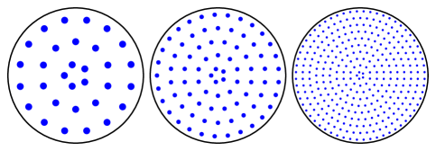
Fubini-Study: $\omega_{FS}$
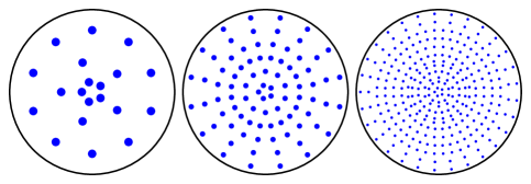
Calabi-Yau: $\Omega\wedge\overline{\Omega}$

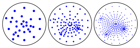
Figure 3: The adaptive mesh generation for four different integrations over the disk $D=\{|z|\leq 1\}$. In each case, the points are chosen such that their weight is approximately constant. The point distributions in the three rows are further explained in items 1, 2, and 3 on page 1.

Note that, by dividing with the homogeneous coordinate of largest magnitude, the homogeneous coordinates of any point can be rescaled such that

• one homogeneous coordinate equals unity, say, $z_{i}=1$, and

• all other homogeneous coordinates have equal or smaller magnitude $|z_{j}|\leq 1$, $j\not=i$.

Hence, a generic point of $\mathop{\hbox{}{\mathbb{P}}}\nolimits^{n}$ is contained in precisely one of the polydiscs $D_{i}$. The polydiscs overlap in the measure-zero set where two or more homogeneous coordinates attain the maximum magnitude.

It remains to decompose each polydisc $D_{i}\simeq D^{n}$. For this purpose, we use that the polydisc is the Cartesian product of $n$ individual disks

$$D=\Big{\{}re^{i\varphi}~{}\Big{|}~{}r\leq 1,\;0\leq\varphi<2\pi\Big{\}}\subset{\mathbb{C}}.$$ (5.5)

Any cell decomposition of $D\subset{\mathbb{C}}$ induces one of the polydisc. For our implementation, we chose to decompose $D$ into annuli of width $\delta r$, and each annulus into segments of angles $\delta\varphi\approx\delta r/(2\pi r)$. The annulus segments are approximately quadratic and of area $2\pi r\delta\varphi\cdot\delta r$ in the Euclidean measure.

To summarize, we decompose the polydiscs $D_{i}$ into hypercubes of constant volume in the Euclidean metric, which we use as the auxiliary measure. If the weight of the cell is too large, we subdivide it by splitting the annulus segment in one of the $n$ discs that constitute $D_{i}$. Summing over each of the $n+1$ polydiscs according to the rectangle rule then computes the integral over $\mathop{\hbox{}{\mathbb{P}}}\nolimits^{n}$. To illustrate the adaptive integration algorithm, we plot the point distribution for three different volume forms in Figure 3. The first, second, and third column shows successive refinements with growing number of points. Each row corresponds to a different volume form that the point distribution is adapted to:

1. In the top row, points are distributed regularly on the disc. This distribution, with constant weight attached to each point, approximates integration with respect to the Euclidean measure.

2. In the second row, we try to approximate integration with respect to the Fubini-Study measure. Here, the points are chosen adaptively and are denser towards the center where the Fubini-Study volume form is denser.

3. In the third row, we illustrate integration over the $(2,2)$-hypersurface

   $$w_{0}^{2}z_{0}^{2}-\tfrac{9+i}{10}w_{0}^{2}z_{0}z_{1}-\tfrac{3-9i}{10}w_{0}^{2}z_{1}^{2}-\tfrac{1-7i}{10}w_{0}w_{1}z_{0}^{2}-\tfrac{5-10i}{10}w_{0}w_{1}z_{0}z_{1}\\ -\tfrac{4-i}{10}w_{0}w_{1}z_{1}^{2}-\tfrac{10+9i}{10}w_{1}^{2}z_{0}^{2}-\tfrac{2+2i}{10}w_{1}^{2}z_{0}z_{1}+\tfrac{5-i}{10}w_{1}^{2}z_{1}^{2}=0$$ (5.6)

   in $\mathop{\hbox{}{\mathbb{P}}}\nolimits^{1}_{[w_{0}:w_{1}]}\times\mathop{\hbox{}{\mathbb{P}}}\nolimits^{1}_{[z_{0}:z_{1}]}$ with respect to the Calabi-Yau volume form. Using the projection $\pi:X\to\mathop{\hbox{}{\mathbb{P}}}\nolimits^{1}_{[z_{0}:z_{1}]}$ we rewrite this integration as the integration over a single $\mathop{\hbox{}{\mathbb{P}}}\nolimits^{1}$. The disc in Figure 3 shows the first patch $[z_{0}:z_{1}]=[z:1]$, $|z|\leq 1$. The points are adaptively chosen to have approximately constant weight.

6 Diagnosing Stability

One of the goals of this paper to use the generalized Donaldson algorithm to probe Kähler cone substructure in higher-dimensional Kähler cones. That is, we would like to efficiently be able to scan a Kähler cone for regions where a given bundle is stable. To this end, we present in this section a new and efficient numerical measure of the stability properties of $\mathscr{V}$ at a fixed polarization.

The central idea is as follows. If one just wants to numerically determine whether a bundle is stable or not, it is not necessary to explicitly compute the Hermitian Yang-Mills connection. Instead, one can simply use the first step of the generalized Donaldson algorithm, namely the convergence properties of the T-operator. As we saw in Subsection 3.2, according to Wang’s theorem, for a fixed embedding defined by $H^{0}(X,\mathscr{V}\otimes{\cal L}^{k_{H}})$, the T-operator can be moved to a balanced place if and only if it is Gieseker stable as defined in eq. (3.20). Thus, for an embedding defined by even a relatively small number of sections (that is, a small degree of twisting $k_{H}$), it should be straightforward to check whether or not the iterations of the T-operator in (3.19) converge to a fixed point. If such a fixed point exists, then we know that the bundle is Giesker stable. In general, this computation is easier and faster than a complete computation of the connection and its integrated error measure.

Figure 4: The T-operator convergence measured for the same bundle and polarizations as in Figure 2.

As part of our program of probing the stability of general bundles $\mathscr{V}$ in higher dimensional Kähler cones, it is intriguing to see that one can gain important information regarding Gieseker stability from the T-operator and only a minimal number of twists $\mathscr{V}\otimes{\cal L}^{k_{H}}$. However, one must be careful. While it is certainly true that all slope-stable bundles are Gieseker stable, properly Gieseker stable bundles need only be slope semi-stable. We can only conclude that if the T-operator fails to converge, then $\mathscr{V}$ is not slope-stable. However, if it does converge, we only know that $\mathscr{V}$ is semi-stable, but not necessarily a solution to (2.1). In order to be certain that $\mathscr{V}$ is properly slope-stable, one would then need to augment the analysis of the T-iteration with a full computation of the $\tau$ error measure in (4.3), as discussed in the previous sections. In the next section, we will investigate this subtle semi-stable behavior in detail. For now, however, we only explore how much can be gained from a simple check of T-operator convergence.

With this idea in mind, we develop a new error measure based on the convergence of the T-operator. Considering the matrix $H_{\alpha\bar{\beta}}$ in (3.22), we would like to know how much the matrix changes as one moves from the $m$-th to the $(m+1)$-th iteration of the T-operator in (3.19). To answer this question, consider the eigenvalues of the $H_{\alpha\bar{\beta}}$-matrix. At each step of the iteration, the largest eigenvalues are the relevant features; small eigenvalues only give small corrections to the connection on the bundle. Let

$$v_{t_{1},t_{2}}^{\text{max}}(m)$$ (6.1)

be the largest eigenvalue of the $H_{\alpha\bar{\beta}}$ after $m$ iterations of the T-operator. Except for the overall numerical scale, one expects that the details of the initial values are washed out by the iteration. However, the overall scale is preserved by the iteration and, moreover, does not enter the connection. Therefore, a good quantity to measure the convergence is

$$r_{(t_{1},t_{2})}^{\text{max}}(m)=\frac{v_{(t_{1},t_{2})}^{\text{max}}(m)}{v_{(t_{1},t_{2})}^{\text{max}}(m-1)}-1.$$ (6.2)

By Theorem 4 and the above considerations, we know that

$$\lim_{m\to\infty}r_{(t_{1},t_{2})}^{\text{max}}(m)=0$$ (6.3)

if $\mathscr{V}$ is Gieseker stable as in eq. (3.20). For the purposes of this paper, we are interested in slope-stability and solutions to the Hermitian Yang-Mills equations. Since slope-stability implies Gieseker stability, it follows that $r_{(t_{1},t_{2})}^{\text{max}}(m)$ should have the following behavior in the presence of Kähler cone substructure:

$$\lim_{m\to\infty}r_{(t_{1},t_{2})}^{\text{max}}(m)\quad\begin{cases}\quad=0&\text{if}~{}(t_{1},t_{2})\in\mathcal{K}_{\text{stable}}\\ \quad>0&\text{if}~{}(t_{1},t_{2})\in\mathcal{K}_{\text{unstable}}\end{cases}$$ (6.4)

We will put this to the test in the example introduced in Subsection 4.2. For the $SU(2)$ bundle $\mathscr{V}$ in (4.5), one would expect

$$\lim_{m\to\infty}r_{(t_{1},t_{2})}^{\text{max}}(m)\quad\begin{cases}\quad=0&\text{if}~{}\frac{t_{1}}{t_{2}}>\frac{4}{3}\\ \quad>0&\text{if}~{}\frac{t_{1}}{t_{2}}<\frac{4}{3}\end{cases}$$ (6.5)

The results are shown in Figure 4 for the same six polarizations chosen in Figure 2. The connection T-operator was computed at $30$ iterations and the comparison of (6.2) made between the $29$th and $30$th iterations. As expected, $r_{(t_{1},t_{2})}^{\text{max}}(30)$ is approximately zero in the slope-stable region of Kähler moduli space, but non-zero in the unstable region.

Figure 5: Convergence of the T-iteration on the $SU(2)$ bundle in (4.5) with substructure for different Kähler moduli. The radial direction $\gcd(t_{1},t_{2})$ is always chosen to be as large as possible subject to the constraint that there are $\dim H^{0}\big{(}\mathscr{O}(t_{1},t_{2})\big{)}\leq 200$ sections.

On the boundary between $\mathcal{K}_{\text{stable}}$ and $\mathcal{K}_{\text{unstable}}$, however, we find that the $r_{(4,3)}^{\text{max}}(30)$ is also close to zero, despite the fact that $\mathscr{V}$ in (4.5) is only slope semi-stable for this polarization. This is to be expected however, since it can be shown via direct computation (and (3.20)) that $\mathscr{V}$ is still properly Gieseker stable for this line in Kähler moduli space and Gieseker stability implies only slope semi-stability. It follows that to accurately determine the behavior on this boundary, one would need to also investigate the $\tau$ error measure of the previous section, which can distinguish between slope-stable and semi-stable behavior. We return to the boundary behavior in the next section.

For now, it should be noted that one need not have checked the T-operator for all $500$ sections in Figure 4. In fact, the convergence of the T-operator is already evident at a much smaller projective embedding. While we must have enough sections to make sure that (3.15) is a proper embedding, we can see the stability properties of $\mathscr{V}$ from the first embedding which makes $H^{0}(X,\mathscr{V}\otimes{\cal L}^{k_{H}})$ non-vanishing. In Figures 5 and 6 we present the same results from a purely “angular” point of view; that is, computing the T-operator at only a single point along each of the rays plotted in Figure 4. These points (that is, the twistings ${\cal L}^{k_{H}}$) were chosen so that there are $\leq 200$ sections at each point. Note that the oscillation in the height of the points in Figure 5 in the unstable region is not significant since we are comparing data from different polarizations, which leads to different normalizations. The only meaningful comparison is between zero and non-zero values of $r_{(t_{1},t_{2})}^{max}(m)$. We also present a $3$-dimensional plot of the same Kähler cone substructure in Figure 6. For all calculations, the connection was computed with $N_{G}=74,892$ points (adaptive) and $30$ iterations of the T-operator.

Figure 6: The Kähler cone substructure associated with the $SU(2)$ bundle in (4.5) for different Kähler moduli. Green points are stable, blue points are on the line of stability, and red points are unstable polarizations.

Finally, in Figure 7 we consider the rate at which the T-operator approaches its fixed point as the number of sections defining the embedding is increased, see eq. (3.15). We observe that convergence of the T-iteration is generally slower for more sections. In particular, in Figure 7 we present the convergence (and divergence) of the T-iteration for polarizations $\mathscr{O}(t,t)$, which is in the unstable region $\mathcal{K}_{\text{unstable}}$ of the Kähler moduli space.

Figure 7: Convergence (for the polarization $\mathscr{O}(2t,t)$) and divergence (for $\mathscr{O}(t,t)$) of the T-iteration on the bundle $\mathscr{V}$ in (4.5). Substructure is shown for different Kähler moduli along a stable and an unstable ray, respectively. The orange and gray lines are associated with two different values of the bundle moduli for the unstable polarization.

7 On The Line Of Semi-Stability

In the previous sections, we demonstrated that the generalized Donaldson algorithm is capable of broadly probing Kähler cone substructure. In this section, we take a detailed look at the boundary between stable/unstable regions, the so-called “stability wall” [39, 40].

Figure 8: The $\tau$ error measure associated with the $SU(2)$ bundle in (4.5) at the stability wall in Kähler moduli space. The bundle modulus $\varphi$ defined in (7.2) determines whether $\mathscr{V}$ is strictly semi-stable (when $\varphi\neq 0$) or poly-stable (when $\varphi=0$). In the latter case, the reducible connection satisfies the Hermitian Yang-Mills equations (2.2).

Let us revisit the $SU(2)$ bundle $\mathscr{V}$ on the $K3$ surface defined by (4.5). As discussed in Subsection 4.2, $\mathscr{V}$ is destabilized in part of the Kähler cone by a rank $1$ subsheaf ${\cal F}\subset\mathscr{V}$ defined in (4.6). In the region $\mathcal{K}_{\text{stable}}$ in (4.7), $\mu({\cal F})<0$ and in $\mathcal{K}_{\text{unstable}}$, $\mu({\cal F})>0$. What happens on the boundary line between these two regions, where $\mu({\cal F})=\mu(\mathscr{V})=0$? By definition, on a line with $\mu({\cal F})=\mu(\mathscr{V})$ the bundle $\mathscr{V}$ is semi-stable. Hence, for generic values of the bundle moduli its connection will not solve the Hermitian Yang-Mills equations. However, semi-stable bundles are distinguished from unstable bundles in that they can provide supersymmetric solutions for special loci in their moduli space. Looking at the definitions in (2.9) and (2.10) in Section 2, we see that the only way that $\mathscr{V}$ can satisfy the Hermitian Yang-Mills equations when $\mu({\cal F})=\mu(\mathscr{V})$ is for it to be poly-stable rather than strictly semi-stable. That is, if the connection on $\mathscr{V}$ is decomposable, it is possible that a connection may exist which satisfies (2.1). Mathematically, this property of slope semi-stable bundles is characterized by the notion of S-equivalence classes and the Harder-Narasimhan filtration [42, 45], which states that every semi-stable bundle has a unique poly-stable representative in its moduli space.

For the bundle in (4.5), we find that the poly-stable representative arises when $\mathscr{V}$ decomposes on the semi-stable wall as the direct sum

$$\mathscr{V}\longrightarrow{\cal F}\oplus{\cal O}(-2,1).$$ (7.1)

Figure 9: The convergence/divergence of T-iteration associated with the $SU(2)$ bundle in (4.5) at the stability wall in Kähler moduli space. The bundle modulus $\varphi$ defined in (7.2) determines whether $\mathscr{V}$ is strictly semi-stable (when $\varphi\neq 0$) or poly-stable (when $\varphi=0$). In the latter case, the reducible connection satisfies the Hermitian Yang-Mills equations (2.2).

One can quantify this decomposable locus in the bundle moduli space as follows. The bundle moduli space of $\mathscr{V}$ is described by the parameters in the map $f$ in (4.5). We can describe the decomposable locus in (7.1) in terms of this map by parametrizing one particular vector bundle modulus as $\varphi$ in the monad map

$$f_{\varphi}=\begin{pmatrix}(9-i)y_{0}+(-6-6i)y_{1}+(-8-8i)y_{2}\\ (-9-9i)y_{0}+(-2+9i)y_{1}+(4-4i)y_{2}\\ \varphi\big{(}{\scriptstyle(-10+7i)x_{0}^{4}+(6-9i)x_{0}^{3}x_{1}+(3-8i)x_{0}^{2}x_{1}^{2}+(-9-4i)x_{0}x_{1}^{3}+(8+4i)x_{1}^{4}}\big{)}\end{pmatrix}$$ (7.2)

which determines $\mathscr{V}_{\varphi}$,

(7.3)

When $\varphi=0$, the bundle splits as in (7.1) and the resulting direct sum is poly-stable and a solution to the Hermitian Yang-Mills equations. When $\varphi\neq 0$, $\mathscr{V}$ is only semi-stable, one cannot solve (2.2), and supersymmetry is broken.

Let us now revisit the numerical results of the past few sections in light of this structure. Can the error measures $\tau(A_{\mathscr{V}})$ and $r^{max}(m)$, introduced in Subsection 4.1 and Section 6 respectively, accurately reveal this $\varphi$-dependent structure? To answer this question, we have run the algorithm for the same bundle again, this time keeping the Kähler moduli fixed directly on the line $(t_{1},t_{2})\sim(4,3)$, but allowing the bundle moduli to vary through the variable $\varphi$. The metric was computed for this polarization with $N_{g}=202,800$ points (adaptive), $30$ iterations of the metric T-operator and with a Kähler form determined by ${\cal O}(4,3)^{\otimes 3}$. Meanwhile, the connection utilized $N_{G}=74,892$ points (adaptive) and $100$ iterations of the connection T-operator. The results for the $\tau(t_{1},t_{2})$ error measure of equation (4.3) are shown in Figure 8. Significantly, the algorithm clearly distinguishes between the semi-stable ($\varphi\neq 0$) and poly-stable ($\varphi=0$) behavior of $\mathscr{V}$. Moreover, one can repeat the same analysis with the T-operator convergence measure, $r^{max}(12,9)(m)$, of (6.2). For this analysis, we hold ourselves fixed at one point in Kähler moduli space ($t_{1}=12,t_{2}=9$) and allowing the number of T-iterations $m$ to increase. Once again, we find that this error measure definitively distinguishes between the supersymmetric and non-supersymmetric configurations. The convergence of the T-iteration is shown in Figure 9.

The graph Figure 9 shows a high degree of sensitivity to the bundle moduli. The fact that the T-iterations can distinguish the $\varphi=0$ and $\varphi\neq 0$ cases is significant, since it means that for a general value of the bundle moduli $\mathscr{V}$ is not Gieseker stable for the boundary wall polarization. This can be verified directly using the destabilizing subsheaf ${\cal F}$ in (4.6) and the definitions of Gieseker stability, (3.20), in Section 2. In fact, for ${\cal L}={\cal O}(4,3)$ we have

$$p_{{\cal L}}({\cal F})(n)=45n^{2}-3,$$ (7.4)

while

$$p_{{\cal L}}(\mathscr{V})(n)=\frac{1}{2}(90n^{2}-8)~{}.$$ (7.5)

Therefore,

$$p_{{\cal L}}(\mathscr{V})(n)\prec p_{{\cal L}}({\cal F})(n)$$ (7.6)

and, by (3.21), $\mathscr{V}$ is not Gieseker stable. The results of Figure 9 are in complete agreement with this; showing the $\varphi=0$ reducible connection T-operator converging to its fixed point while the Gieseker unstable configurations with $\varphi\neq 0$ fail to converge. It follows that the T-operator is sensitive enough to the bundle moduli that it can distinguish between these important cases.

8 A Calabi-Yau Threefold Example

In the previous sections, we investigated Kähler cone substructure with a number of new tools and from a variety of perspectives. Here, we present a final example involving geometry directly relevant to realistic $\mathcal{N}=1$ heterotic compactifications; namely, a Calabi-Yau threefold with a higher-rank vector bundle defined over it.

As a base manifold, we choose a Calabi-Yau threefold determined by a generic degree $(4,2)$-hypersurface in $\mathop{\hbox{}{\mathbb{P}}}\nolimits^{3}\times\mathop{\hbox{}{\mathbb{P}}}\nolimits^{1}$. For this threefold, $h^{1,1}=2$ and all line bundles can be written in the form ${\cal O}(a_{1},a_{2})$, where ${\cal O}(1,0)$ arises from the hyperplane descending from $\mathbb{P}^{1}$ and ${\cal O}(0,1)$ descends from the hyperplane of $\mathbb{P}^{3}$.

Figure 10: Convergence of the T-iteration on the $SU(3)$ bundle defined by (8.2) for different Kähler moduli. The radial direction $\gcd(t_{1},t_{2})$ is always chosen to be as large as possible subject to the constraint that there are $\dim H^{0}\big{(}\mathscr{O}(t_{1},t_{2})\big{)}\leq 500$ sections. The results agree with the Kähler cone substructure in (8.4).

Over this threefold, define the $SU(3)$ monad bundle

$$0\longrightarrow\mathscr{V}\longrightarrow{\cal O}(-2,1)\oplus{\cal O}(3,-1)\oplus{\cal O}(2,0)\oplus{\cal O}(2,1)^{\oplus 2}\stackrel{{\scriptstyle f}}{{\longrightarrow}}{\cal O}(4,1)\oplus{\cal O}(3,1)\longrightarrow 0$$ (8.1)

and its associated dual bundle

$$0\longrightarrow{\cal O}(-4,-1)\oplus{\cal O}(-3,-1)\longrightarrow\\ {\cal O}(-2,-1)^{\oplus 2}\oplus{\cal O}(-2,0)\oplus{\cal O}(-3,1)\oplus{\cal O}(2,-1)\longrightarrow\mathscr{V}^{\vee}\longrightarrow 0.$$ (8.2)

This example was chosen because it once again the stability depends on the precise value of the Kähler moduli. It can be verified, using the definitions of Section 2, that the bundle $\mathscr{V}$ in eq. (8.1) has two potentially destabilizing sub-sheaves. These are ${\cal F}_{1}$,${\cal F}_{2}\subset\mathscr{V}$ given by

$$\begin{split}&0\longrightarrow{\cal F}_{1}\longrightarrow{\cal O}(3,-1)\oplus{\cal O}(2,0)\oplus{\cal O}(2,1)^{\oplus 2}\stackrel{{\scriptstyle f}}{{\longrightarrow}}{\cal O}(4,1)\oplus{\cal O}(3,1)\longrightarrow 0,\\ &0\longrightarrow{\cal F}_{2}\longrightarrow{\cal O}(-2,1)\oplus{\cal O}(2,0)\oplus{\cal O}(2,1)^{\oplus 2}\stackrel{{\scriptstyle f}}{{\longrightarrow}}{\cal O}(4,1)\oplus{\cal O}(3,1)\longrightarrow 0.\end{split}$$ (8.3)

Both are of rank $2$ with $c_{1}({\cal F}_{1})=(2,-1)$ and $c_{1}({\cal F}_{2})=(-3,1)$. Due to these two destabilizing sub-sheaves, the Kähler cone divides into three regions

$$\begin{split}\mathcal{K}_{\text{stable}}=&\;\big{\{}\mathscr{O}(t_{1},t_{2})\;\big{|}\;\tfrac{4}{5}<\tfrac{t_{2}}{t_{1}}<\tfrac{4}{3}\big{\}},\\ \mathcal{K}_{\text{unstable}}=&\;\big{\{}\mathscr{O}(t_{1},t_{2})\;\big{|}\;\tfrac{t_{2}}{t_{1}}<\tfrac{4}{5}\big{\}}~{}\cup~{}\big{\{}\mathscr{O}(t_{1},t_{2})\;\big{|}\;\tfrac{t_{2}}{t_{1}}>\tfrac{4}{3}\big{\}}.\end{split}$$ (8.4)

Moreover, a direct calculation using (3.20) shows that $\mathscr{V}$ is still Gieseker stable at each of the stability walls defined by $t_{2}/t_{1}=4/3$ and $t_{2}/t_{1}=4/5$. Thus, while the bundle is strictly semi-stable along these rays (and, hence, does not solve the Hermitian Yang-Mills equations eq. (2.2)), one would still expect the T-iteration to converge for points along these boundaries.

For ease of embedding, the T-operator is computed for $\mathscr{V}^{\vee}$. However, since $\mathscr{V}$ and its dual must be slope-stable/unstable in the same regions of Kähler moduli space, this does not affect our results. Since we have demonstrated in the previous sections that the T-iteration is a fast and efficient check of stability, we will consider here only the error measure $r_{(t_{1},t_{2})}^{max}(m)$. It is interesting to observe that, even in this more complex example, the data shown in Figure 10 clearly reproduces the Kähler cone substructure described in (8.4). Moreover, at the points on the two stability walls we find, as expected, that $r_{(t_{1},t_{2})}^{max}(30)=0$, since $\mathscr{V}$ is still Gieseker stable for these lines of slope semi-stability. The connection integration was performed with $N_{G}=119,164$ points (adaptive) and $30$ iterations of the T-operator. The plot shown in Figure 10 are analogous to the results in Figure 5 for the $K3$ surface.

9 Conclusions and Future Work

In this paper, we extended the generalized Donaldson algorithm to manifolds with higher-dimensional Kähler cones and presented a method for approximating the connection on slope-stable holomorphic vector bundles in this context. We also introduced a numerical criterion for determining the existence of supersymmetric heterotic vacua, without having to compute the connection. These techniques clearly can be used to search for new classes of smooth $\mathcal{N}=1$ supersymmetric vacua in heterotic string theory. However, the explicit knowledge of the gauge connection that they provide allows us to go far beyond a simple categorization of vacua.

It is a long-standing goal of string theory to produce low-energy theories whose effective actions reproduce the symmetries, particle spectrum, and properties of elementary particle physics. Within the context of smooth heterotic string or M-theory compactifications [2, 7, 60], there has been considerable progress in recent years [61, 62, 63, 64, 65, 66, 53]. Despite these successes, certain observable quantities of particle physics, such as the gauge and Yukawa couplings, are difficult to compute directly. Normalized Yukawa couplings, for example, depend on both the coefficients of cubic terms in the superpotential and the explicit form of the Kähler potential. In turn, these quantities depend on the detailed structure of the underlying geometry – that is, the metric and gauge connection on the Calabi-Yau threefold and holomorphic vector bundle respectively. Hence, the Yukawa couplings in the four-dimensional effective theory are not known, except in very special cases. One can rarely do better than the qualitative statement that such coupling coefficents either vanish or are of order one. However, the methods introduced in [32, 29] and extended in this paper allow one, for the first time, to explicitly compute both the metric and the gauge connection and, hence, the Yukawa coefficients. In future work [67], we will use these techniques to calculate these physical couplings.

Bibliography

- [1] D. J. Gross, J. A. Harvey, E. J. Martinec, and R. Rohm, “The Heterotic String,” Phys. Rev. Lett. 54 (1985) 502–505.
- [2] P. Candelas, G. T. Horowitz, A. Strominger, and E. Witten, “Vacuum Configurations for Superstrings,” Nucl. Phys. B258 (1985) 46–74.
- [3] P. Horava and E. Witten, “Heterotic and type I string dynamics from eleven dimensions,” Nucl. Phys. B460 (1996) 506–524, hep-th/9510209.
- [4] P. Horava and E. Witten, “Eleven-Dimensional Supergravity on a Manifold with Boundary,” Nucl. Phys. B475 (1996) 94–114, hep-th/9603142.
- [5] E. Witten, “Strong Coupling Expansion Of Calabi-Yau Compactification,” Nucl. Phys. B471 (1996) 135–158, hep-th/9602070.
- [6] A. Lukas, B. A. Ovrut, and D. Waldram, “On the four-dimensional effective action of strongly coupled heterotic string theory,” Nucl. Phys. B532 (1998) 43–82, hep-th/9710208.
- [7] A. Lukas, B. A. Ovrut, K. S. Stelle, and D. Waldram, “The universe as a domain wall,” Phys. Rev. D59 (1999) 086001, hep-th/9803235.
- [8] A. Lukas, B. A. Ovrut, K. S. Stelle, and D. Waldram, “Heterotic M-theory in five dimensions,” Nucl. Phys. B552 (1999) 246–290, hep-th/9806051.
- [9] M. B. Green, J. H. Schwarz, and E. Witten, “SUPERSTRING THEORY. VOL. 1: INTRODUCTION,”. Cambridge, Uk: Univ. Pr. (1987) 469 P. (Cambridge Monographs On Mathematical Physics).
- [10] S. T. Yau, “On the Ricci curvature of a compact Kähler manifold and the complex Monge-Ampère equation. I,” Comm. Pure Appl. Math. 31 (1978), no. 3, 339–411.
- [11] K. Uhlenbeck and S.-T. Yau., “On the existence of Hermitian Yang-Mills connections in stable bundles,” Comm. Pure App. Math. 39 (1986) 257.
- [12] S. Donaldson, “Anti Self-Dual Yang-Mills Connections over Complex Algebraic Surfaces and Stable Vector Bundles,,” Proc. London Math. Soc. 3 (1985) 1.
- [13] P. Candelas and S. Kalara, “Yukawa couplings for a three generation superstring compactification,” Nucl. Phys. B298 (1988) 357.
- [14] P. Candelas, X. C. De La Ossa, P. S. Green, and L. Parkes, “A pair of Calabi-Yau manifolds as an exactly soluble superconformal theory,” Nucl. Phys. B359 (1991) 21–74.
- [15] B. R. Greene, D. R. Morrison, and M. R. Plesser, “Mirror manifolds in higher dimension,” Commun. Math. Phys. 173 (1995) 559–598, hep-th/9402119.
- [16] R. Donagi, R. Reinbacher, and S.-T. Yau, “Yukawa couplings on quintic threefolds,” hep-th/0605203.
- [17] V. Braun, Y.-H. He, and B. A. Ovrut, “Yukawa couplings in heterotic standard models,” JHEP 04 (2006) 019, hep-th/0601204.
- [18] L. B. Anderson, J. Gray, D. Grayson, Y.-H. He, and A. Lukas, “Yukawa Couplings in Heterotic Compactification,” Commun. Math. Phys. 297 (2010) 95–127, 0904.2186.
- [19] S. K. Donaldson, “Scalar curvature and projective embeddings. II,” Q. J. Math. 56 (2005), no. 3, 345–356.
- [20] S. K. Donaldson, “Scalar curvature and projective embeddings. I,” J. Differential Geom. 59 (2001), no. 3, 479–522.
- [21] S. K. Donaldson, “Some numerical results in complex differential geometry,” math.DG/0512625.
- [22] G. Tian, “On a set of polarized Kähler metrics on algebraic manifolds,” J. Differential Geom. 32 (1990), no. 1, 99–130.
- [23] X. Wang, “Canonical metrics on stable vector bundles,” Comm. Anal. Geom. 13 (2005), no. 2, 253–285.
- [24] M. R. Douglas, R. L. Karp, S. Lukic, and R. Reinbacher, “Numerical solution to the hermitian Yang-Mills equation on the Fermat quintic,” hep-th/0606261.
- [25] M. Headrick and T. Wiseman, “Numerical Ricci-flat metrics on ,” Classical Quantum Gravity 22 (2005), no. 23, 4931–4960.
- [26] C. Doran, M. Headrick, C. P. Herzog, J. Kantor, and T. Wiseman, “Numerical Kaehler-Einstein metric on the third del Pezzo,” hep-th/0703057.
- [27] M. Headrick and A. Nassar, “Energy functionals for Calabi-Yau metrics,” 0908.2635.
- [28] M. R. Douglas and S. Klevtsov, “Black holes and balanced metrics,” 0811.0367.
- [29] L. B. Anderson, V. Braun, R. L. Karp, and B. A. Ovrut, “Numerical Hermitian Yang-Mills Connections and Vector Bundle Stability in Heterotic Theories,” JHEP 06 (2010) 107, 1004.4399.
- [30] V. Braun, T. Brelidze, M. R. Douglas, and B. A. Ovrut, “Calabi-Yau Metrics for Quotients and Complete Intersections,” arXiv:0712.3563 [hep-th].
- [31] V. Braun, T. Brelidze, M. R. Douglas, and B. A. Ovrut, “Eigenvalues and Eigenfunctions of the Scalar Laplace Operator on Calabi-Yau Manifolds,” JHEP 07 (2008) 120, 0805.3689.
- [32] M. R. Douglas, R. L. Karp, S. Lukic, and R. Reinbacher, “Numerical Calabi-Yau metrics,” hep-th/0612075.
- [33] R. Seyyedali, “Numerical Algorithms for Finding Balanced Metrics on Vector Bundles,” ArXiv e-prints (Apr., 2008) 0804.4005.
- [34] J. Keller, “Ricci iterations on Kahler classes,” ArXiv e-prints (Sept., 2007) 0709.1490.
- [35] D. H. Phong and J. Sturm, “Stability, energy functionals, and K”ahler-Einstein metrics,” ArXiv Mathematics e-prints (Mar., 2002) arXiv:math/0203254.
- [36] H. S. C. Okonek, M. Schneider, Vector Bundles on Complex Projective Spaces. Birkhauser Verlag, 1988.
- [37] L. B. Anderson, Y.-H. He, and A. Lukas, “Heterotic compactification, an algorithmic approach,” JHEP 07 (2007) 049, hep-th/0702210.
- [38] L. B. Anderson, Y.-H. He, and A. Lukas, “Monad Bundles in Heterotic String Compactifications,” JHEP 07 (2008) 104, 0805.2875.
- [39] L. B. Anderson, J. Gray, A. Lukas, and B. Ovrut, “The Edge Of Supersymmetry: Stability Walls in Heterotic Theory,” Phys. Lett. B677 (2009) 190–194, 0903.5088.
- [40] L. B. Anderson, J. Gray, A. Lukas, and B. Ovrut, “Stability Walls in Heterotic Theories,” JHEP 09 (2009) 026, 0905.1748.
- [41] R. Blumenhagen, S. Moster, and T. Weigand, “Heterotic GUT and Standard Model vacua from simply connected Calabi-Yau manifolds,” hep-th/0603015.
- [42] D. Huybrechts and M. Lehn, “The geometry of the Moduli Spaces of Sheaves,” Aspects of Mathematics E 31 (1997).
- [43] Y. Sano, “Numerical algorithm for finding balanced metrics,” Osaka J. Math. 43 (2006), no. 3, 679–688.
- [44] P. Griffiths and J. Harris, Principles of algebraic geometry. Wiley-Interscience [John Wiley & Sons], New York, 1978. Pure and Applied Mathematics.
- [45] J. Keller, “Canonical metrics and Harder-Narasimhan filtration,” in Contemporary aspects of complex analysis, differential geometry and mathematical physics, pp. 132–148. World Sci. Publ., Hackensack, NJ, 2005.
- [46] E. R. Sharpe, “Kaehler cone substructure,” Adv. Theor. Math. Phys. 2 (1999) 1441–1462, hep-th/9810064.
- [47] L. B. Anderson, J. Gray, and B. Ovrut, “Yukawa Textures From Heterotic Stability Walls,” JHEP 05 (2010) 086, 1001.2317.
- [48] L. B. Anderson, J. Gray, A. Lukas, and B. Ovrut, “Stabilizing the Complex Structure in Heterotic Calabi-Yau Vacua,” JHEP 02 (2011) 088, 1010.0255.
- [49] L. B. Anderson, J. Gray, A. Lukas, and B. Ovrut, “Stabilizing All Geometric Moduli in Heterotic Calabi-Yau Vacua,” 1102.0011.
- [50] R. P. Thomas, “A holomorphic Casson invariant for Calabi-Yau 3-folds, and bundles on K3 fibrations,” math/9806111.
- [51] W. Li and Z. Qin, “Donaldson-Thomas invariants of certain Calabi-Yau 3-folds,” ArXiv e-prints (Feb., 2010) 1002.4080.
- [52] L. B. Anderson, J. Gray, and B. Ovrut, “Transitions in the Web of Heterotic Vacua,” 1012.3179.
- [53] L. B. Anderson, J. Gray, Y.-H. He, and A. Lukas, “Exploring Positive Monad Bundles And A New Heterotic Standard Model,” JHEP 02 (2010) 054, 0911.1569.
- [54] L. B. Anderson, “Heterotic and M-theory Compactifications for String Phenomenology,” 0808.3621.
- [55] S. K. Donaldson, “Some numerical results in complex differential geometry,” ArXiv Mathematics e-prints (Dec., 2005) arXiv:math/0512625.
- [56] R. S. Bunch and S. K. Donaldson, “Numerical approximations to extremal metrics on toric surfaces,” ArXiv e-prints (Mar., 2008) 0803.0987.
- [57] B. Shiffman and S. Zelditch, “Distribution of zeros of random and quantum chaotic sections of positive line bundles,” Comm. Math. Phys. 200 (1999), no. 3, 661–683.
- [58] S. Zelditch, “Szegő kernels and a theorem of Tian,” Internat. Math. Res. Notices (1998), no. 6, 317–331.
- [59] J. Keller and S. Lukic, “Numerical Weil-Petersson metrics on moduli spaces of Calabi-Yau manifolds,” 0907.1387.
- [60] A. Lukas, B. A. Ovrut, and D. Waldram, “The ten-dimensional effective action of strongly coupled heterotic string theory,” Nucl. Phys. B540 (1999) 230–246, hep-th/9801087.
- [61] V. Braun, B. A. Ovrut, T. Pantev, and R. Reinbacher, “Elliptic Calabi-Yau threefolds with Z(3) x Z(3) Wilson lines,” JHEP 12 (2004) 062, hep-th/0410055.
- [62] V. Braun, Y.-H. He, B. A. Ovrut, and T. Pantev, “The exact MSSM spectrum from string theory,” JHEP 05 (2006) 043, hep-th/0512177.
- [63] V. Braun, Y.-H. He, B. A. Ovrut, and T. Pantev, “A heterotic standard model,” Phys. Lett. B618 (2005) 252–258, hep-th/0501070.
- [64] V. Braun, Y.-H. He, B. A. Ovrut, and T. Pantev, “Vector bundle extensions, sheaf cohomology, and the heterotic standard model,” Adv. Theor. Math. Phys. 10 (2006) 4, hep-th/0505041.
- [65] E. I. Buchbinder, J. Khoury, and B. A. Ovrut, “New Ekpyrotic Cosmology,” Phys. Rev. D76 (2007) 123503, hep-th/0702154.
- [66] V. Bouchard and R. Donagi, “An SU(5) heterotic standard model,” Phys. Lett. B633 (2006) 783–791, hep-th/0512149.
- [67] L. B. Anderson, V. Braun, and B. A. Ovrut, “Numerical determination of Yukawa couplings.” To appear.