Quantum computation with prethreshold superconducting qubits: Single-excitation subspace approach

Abstract

We describe an alternative approach to quantum computation that is ideally suited for today’s sub-threshold-fidelity qubits, and which can be applied to a family of hardware models that includes superconducting qubits with tunable coupling. In this approach, the computation on an $n$-qubit processor is carried out in the $n$-dimensional single-excitation subspace (SES) of the full $2^{n}$-dimensional Hilbert space. Because any real Hamiltonian can be directly generated in the SES [E. J. Pritchett et al., arXiv:1008.0701], high-dimensional unitary operations can be carried out in a single step, bypassing the need to decompose into single- and two-qubit gates. Although technically nonscalable and unsuitable for applications (including Shor’s) requiring enormous Hilbert spaces, this approach would make practical a first-generation quantum computer capable of achieving significant quantum speedup.

I Introduction

In the standard gate-based model of quantum computation with $n$ qubits, the initial state of the (closed) system is represented by a $2^{n}$-dimensional complex vector $\psi$, and the computation is described by a unitary time-evolution operator $U$. Running the quantum computer implements the map

$$\psi\rightarrow U\psi.$$ (1)

A key feature of this approach to quantum information processing is the exponential classical information storage capacity of the wave function $\psi$. However, the number of one- and two-qubit gates required to implement an arbitrary element of the unitary group ${\rm U}(2^{n})$ is at least $2^{2n}$, making the construction of an arbitrary $U$ inefficient (using elementary gates). The goal of quantum algorithm design is to compute interesting cases of $U$ with a polynomial number of elementary gates; two important examples are the algorithms for factoring Shor (1997) and quantum simulation Lloyd (1996). Although these algorithms are efficient, the number of gates required for interesting applications is still large and error-corrected qubits are therefore required Neilsen and Chuang (2000).

Central to this gate (or quantum circuit) model of quantum computation is the idea that a set of elementary one- and two-qubit gates can be used to construct an arbitrary high-dimensional $U$. But why should we use such a decomposition in the first place? The reason is that the Hamiltonians nature usually provides for us have one- and two-qubit terms (one-body and two-body operators). Consider, for example, the following somewhat generic solid-state model of an array of $n$ coupled qubits,

$$H_{\rm qc}=\sum_{i}\epsilon_{i}c_{i}^{\dagger}c_{i}+\sum_{i<j}g_{ij}\,J_{\mu\nu}\,\sigma^{\mu}_{i}\otimes\sigma^{\nu}_{j},$$ (2)

written in the basis of uncoupled-qubit eigenstates not . Here $i,j=1,2,\dots,n,$ and $\mu,\nu=x,y,z.$ The $\epsilon_{i}$ are the uncoupled qubit energies, $g_{ij}$ (with $i\neq j$) are qubit-qubit interaction strengths, and $J_{\mu\nu}$ is a fixed dimensionless tensor determined by the hardware.

It is clear from (2) that one- and two-qubit operations are naturally generated in this system, and we know (from universality Lloyd (1995); Barenco et al. (1995)) that this is sufficient. If the hardware also provided controllable terms of the form

$$\sum_{ijk}g_{ijk}\,J_{\mu\nu\lambda}\sigma^{\mu}_{i}\otimes\sigma^{\nu}_{j}\otimes\sigma^{\lambda}_{k},$$ (3)

then three-qubit gates could be used as primitives as well.

II QUANTUM COMPUTATION IN THE SES

The idea we explore here is to perform a quantum computation in the $n$-dimensional single-excitation subspace (SES) of the full $2^{n}$-dimensional Hilbert space. This is the subspace spanned by the computational basis states

$$|m)\equiv c_{m}^{\dagger}|00\cdots 0\rangle=|0\cdots 1_{m}\cdots 0\rangle,$$ (4)

with $m=1,2,\dots,n.$ Experimentally, it is possible to prepare the quantum computer in the SES, and it will remain there with high probability as long as (i) the coupling strengths $|g_{ij}|$ are much smaller than the $\epsilon_{i}$; and (ii) certain single-qubit operations such as $\pi$ pulses are not used (however, $2\pi$ pulses are permitted and turn out to be extremely useful, and $\pi$ pulses can be used to prepare SES states from the ground state $|00\cdots 0\rangle$).

The advantage of working in the SES can be understood from the following expression Pritchett et al. ; mat for the SES matrix elements of model (2),

$$\big{(}m\big{|}H_{\rm qc}\big{|}m^{\prime}\big{)}=\bigg{[}\epsilon_{m}-2J^{zz}\big{(}\sum_{k<m}g_{km}+\sum_{k>m}g_{mk}\big{)}+J^{zz}\big{(}\sum_{i<j}g_{ij}\big{)}\bigg{]}\delta_{mm^{\prime}}+\bigg{[}J^{xx}+J^{yy}-i(J^{xy}-J^{yx})\bigg{]}g_{mm^{\prime}}.$$ (5)

Therefore, we have a high degree of control over the part of the Hamiltonian in the SES. For example, in the simple case of an array of qubits coupled with a tunable $\sigma^{x}_{i}\otimes\sigma^{x}_{j}$ exchange interaction,

$$\big{(}m\big{|}H_{\rm qc}\big{|}m^{\prime}\big{)}=\epsilon_{m}\delta_{mm^{\prime}}+g_{mm^{\prime}},$$ (6)

so the diagonal and off-diagonal elements are directly and independently controlled by the qubit energies and coupling strengths, respectively. Because of this high degree of controllability, $n$-dimensional unitary operations can be carried out in a single step, bypassing the need to decompose into elementary gates. This property also enables the direct quantum simulation of real but otherwise arbitrary time-dependent Hamiltonians, allowing a polynomial quantum speedup with sub-threshold-fidelity qubits Pritchett et al. .

A quantum computer operating in the SES mode described here requires every qubit to be tunably coupled to the others, as implied by model (2). This requires $n(n-1)/2$ coupling wires and associated circuits. Consider, for example, the recently demonstrated tunable inductive coupler for superconducting phase qubits Pinto et al. (2010); Bialczak et al. (2011) (other tunable couplers for superconducting qubits have also been successfully demonstrated van der Ploeg et al. (2007); Niskanen et al. (2007); Yamamoto et al. (2008); Allman et al. (2010)). The circuit diagrams for a single phase qubit “q” and single coupler “c” are illustrated in Fig. 1, where the crossed boxes represent Josephson junctions. In terms of these elements, a possible layout for a fully connected array is shown in Fig. 2 for the case of $n=5$.

The SES computation method is not scalable, because it requires a qubit for every Hilbert space dimension used. However the advantage is that high-dimensional unitary operations can be carried out in a single step without the need to decompose the operation into elementary gates. This property allows processors of even modest sizes to perform quantum computations that would otherwise (using a gate-based approach) require thousands of elementary gates and therefore error-corrected qubits. In the remainder of this paper, we illustrate the SES computation method by applying it to Grover’s search algorithm Grover (1997).

III application to Grover’s search algorithm

Here we consider the search for a single marked item in a database of size $n$, where $n$ is the number of qubits in the SES processor (2). Within the SES, Grover’s algorithm Grover (1997) is represented by the following control sequence,

$$\big{(}{W}{\rm O}_{m^{\prime}}\big{)}^{n_{\rm Grover}}U_{\rm unif}|1)\approx|m^{\prime}),$$ (7)

where $U_{\rm unif}$ generates the uniform superposition of all SES states $|m)$, $m=1,2,\dots,n$. Here ${\rm O}_{m^{\prime}}$ is the oracle corresponding to the marked state $|m^{\prime})$, $W$ is Grover’s inversion operator, and $n_{\rm Grover}\approx(\pi/4)\sqrt{n}$ is the number of iteration steps of the algorithm. In the following sections we show how each of these unitary operators can be generated in a single step.

III.1 Preparation of the uniform state

The uniform superposition state,

$$|\psi_{\rm unif})\equiv\frac{1}{\sqrt{n}}\sum_{m=1}^{n}|m)=\frac{1}{\sqrt{n}}\begin{bmatrix}1&1&1&1&\dots\end{bmatrix}^{\rm T},$$ (8)

can be generated from the state $|1)=\begin{bmatrix}1&0&0&0&\dots\end{bmatrix}^{\rm T}$, where ^T stands for transposition, through

$$|\psi_{\rm unif})=ie^{i\alpha_{\rm unif}}e^{-iH_{\rm unif}t_{\rm unif}}|1),$$ (9)

with

$$\alpha_{\rm unif}=\pi/(2\sqrt{n})$$ (10)

and

$$t_{\rm unif}=\pi/(2g\sqrt{n}),$$ (11)

using the SES Hamiltonian

$$H_{\rm unif} = g\begin{bmatrix}2&1&1&1&\dots\cr 1&0&0&0&\dots\cr 1&0&0&0&\dots\cr 1&0&0&0&\dots\cr\vdots&\vdots&\vdots&\vdots&\ddots\cr\end{bmatrix}.$$ (12)

This can be seen by noticing that the spectrum of $H_{\rm unif}$ and the transformation $S$ (whose columns are shown unnormalized here for notational simplicity) that diagonalizes $H_{\rm unif}$ via $H_{\rm unif}^{\rm diag}=S^{\dagger}H_{\rm unif}S$ are given by

$$E=1\mp\sqrt{N},0,\dots,0,$$ (13)

and

$$S=\begin{pmatrix}1-\sqrt{N}&1+\sqrt{N}&0&0&0&\dots&0\cr 1&1&-1&-1&-1&\dots&-1\cr 1&1&1&0&0&\dots&0\cr 1&1&0&1&0&\dots&0\cr 1&1&0&0&1&\dots&0\cr\vdots&\vdots&\vdots&\vdots&\vdots&\ddots&\vdots\cr 1&1&0&0&0&\dots&1\end{pmatrix},$$ (14)

respectively. Direct exponentiation then immediately leads to Eq. (9). The initial state $|1)$ required in (9) is easily prepared from the ground state via a $\pi$ pulse.

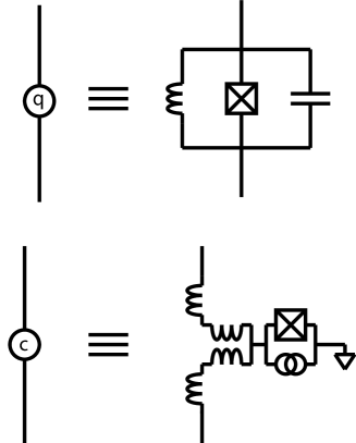
Figure 1: Definitions of two-terminal phase qubit circuit element “q” and coupler circuit element“c”, expressed in terms of their conventional circuit diagrams involving inductors, capacitors, current biases, and Josephson junctions (crossed boxes) Pinto et al. (2010); Bialczak et al. (2011).

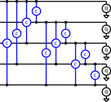
Figure 2: (color online) Design for a fully connected network of $n$ Josephson phase qubits. Each qubit “q” is suplied with a wire to which $n-1$ coupler leads are attached. The case of $n=5$ is shown. The proposed design minimizes crossovers.

III.2 Single-step oracle and $W$ operators

The oracle (corresponding to the marked state with $m^{\prime}=3$, for instance), is

$${\rm O} = 1-2|m^{\prime})(m^{\prime}|=\begin{bmatrix}1&0&0&0&\dots\cr 0&1&0&0&\dots\cr 0&0&-1&0&\dots\cr 0&0&0&1&\dots\cr\vdots&\vdots&\vdots&\vdots&\ddots\cr\end{bmatrix},$$ (15)

which can be generated via

$$W=e^{-iH_{\rm O}t_{\rm O}},\quad t_{\rm O}=\pi/\delta\epsilon,$$ (16)

using the SES Hamiltonian

$$H_{\rm O} = \begin{bmatrix}0&0&0&0&\dots\cr 0&0&0&0&\dots\cr 0&0&-\delta\epsilon&0&\dots\cr 0&0&0&0&\dots\cr\vdots&\vdots&\vdots&\vdots&\ddots\cr\end{bmatrix}.$$ (17)

$\delta\epsilon$ is the detuning of qubit $m^{\prime}$ from the remaining qubits, all having common frequency $\epsilon$. This operation is simply a $2\pi$ rotation on the qubit associated with the marked state $m^{\prime}$. (Although we have implemented it as a $z$ rotation, an $x$ or $y$ rotation would work equally well.) Notice that in the limit $g\ll\epsilon$, which guarantees good isolation of the SES, the oracle can be made arbitrarily fast if we choose sufficiently large detuning $\delta\epsilon$.

Finally, the $W$ operator,

$${\rm W} = 2|\psi_{\rm unif})(\psi_{\rm unif}|-1$$ (18)

$$= \frac{1}{n}\begin{bmatrix}2-n&2&2&2&\dots\cr 2&2-n&2&2&\dots\cr 2&2&2-n&2&\dots\cr 2&2&2&2-n&\dots\cr\vdots&\vdots&\vdots&\vdots&\ddots\cr\end{bmatrix},$$

can be generated via

$${\rm W}=e^{-i\alpha_{\rm W}}e^{-iH_{\rm W}t_{\rm W}},$$

$$\alpha_{\rm W}=(1-n)\pi/n,\quad t_{\rm W}=\pi/(ng),$$ (19)

with

$$H_{\rm W} = g\begin{bmatrix}0&1&1&1&\dots\cr 1&0&1&1&\dots\cr 1&1&0&1&\dots\cr 1&1&1&0&\dots\cr\vdots&\vdots&\vdots&\vdots&\ddots\cr\end{bmatrix}.$$ (20)

III.3 Comparison with gate-based computation

Here we compare the SES and conventional gate-based approaches for a $n=256$ item search. The search requires 12 iterations.

In the SES case, we choose a weak, $g/2\pi=1.25$ MHz coupling, which guarantees that the $W$ operation is at least 1.5 ns long. We also choose a strong, $\delta\epsilon/2\pi=100$ MHz qubit detuning to guarantee that the oracle is sufficiently fast. Then $t_{\rm unif}=12.5$ ns, $t_{\rm O}=5$ ns, $t_{\rm W}=1.56$ ns, and the total duration of the algorithm is about 100 ns, which is experimentally practical with current superconducting architectures.

The SES estimate should be contrasted with the conventional approach, which requires an input register of 8 qubits, an output register of 1 qubit, plus 7 additional ancilla qubits (to make the multiply controlled gates more efficient). The corresponding search oracle involves an 8-fold CNOT gate, ${\rm C}^{8}{\rm NOT}$, each of which can be made out of 85 two-qubit CNOTs (using 7 ancillas) Neilsen and Chuang (2000). The $W$ operator involves a 7-fold controlled-Z gate, ${\rm C}^{7}{\rm Z}$, which uses 73 standard CNOTs (plus 6 ancillas). Thus, a conventional 256-item gate-based Grover search requires 158 CNOT gates per search step. The full algorithm then contains nearly 2000 CNOT gates, plus local rotations.

IV discussion

We have described an approach to superconducting quantum computation in which the computation is carried out in the single-excitation subspace of the full Hilbert space. Relative to the standard gate-based approach, the SES method requires exponentially more qubits and is therefore nonscalable. The hardware requirements are also highly demanding: The fully connected array of $n$ qubits requires $n(n-1)/2$ coupling wires and tuning circuits. But the SES approach is much more time efficient, permitting far larger computations than currently possible using today’s sub-theshold-fidelity qubits in the standard way. This was illustrated above for Grover’s search algorithm. We would expect a similar result for Shor’s algorithm, but note that practical factoring applications would require impossibly large processor sizes. General purpose time-dependent quantum simulation can also be carried out in the SES, allowing an $n^{3}$ polynomial quantum speedup Pritchett et al. . However, when a large scale error-corrected quantum computer eventually becomes available, the gate-based approach will perform better than the SES method.