Fidelity decay in interacting two-level boson systems: Freezing and revivals

Abstract

We study the fidelity decay in the $k$-body embedded ensembles of random matrices for bosons distributed in two single-particle states, considering the reference or unperturbed Hamiltonian as the one-body terms and the diagonal part of the $k$-body embedded ensemble of random matrices, and the perturbation as the residual off-diagonal part of the interaction. We calculate the ensemble-averaged fidelity with respect to an initial random state within linear response theory to second order on the perturbation strength, and demonstrate that it displays the freeze of the fidelity. During the freeze, the average fidelity exhibits periodic revivals at integer values of the Heisenberg time $t_{H}$. By selecting specific $k$-body terms of the residual interaction, we find that the periodicity of the revivals during the freeze of fidelity is an integer fraction of $t_{H}$, thus relating the period of the revivals with the range of the interaction $k$ of the perturbing terms. Numerical calculations confirm the analytical results.

I Introduction

Fidelity, or Loschmidt echo, was introduced to study the effect of perturbations on the dynamics of quantum systems, mainly in the context of quantum information, but also in the study of the stability of quantum systems; for a review see Gorin2006 . Prosen and Žnidarič noted that a freeze of fidelity occurs, i.e. fidelity will remain stable for very long times in the scale of the Heisenberg time, if the diagonal part of the perturbation matrix vanishes ProsenZnid2003 . This lead to an additional interesting view on fidelity decay. In any given system, we can view any part of the Hamiltonian as the unperturbed system and the rest as perturbation. In particular in a many-body system the mean-field theory can be considered to be the unperturbed system, and the residual interaction as the perturbation. Fidelity thus serves as a measure of the quality of such mean-field approach. This was actually considered in Ref. Pizorn2007 in the context of a random matrix model using a two-body random ensemble, i.e. an ensemble that takes into account the two-body character of the interactions as well as the fermionic character of the particles. The result was rather surprising in the sense, that the freeze does not occur for the ensemble-average of fidelity, but it does occur for the median fidelity, or equivalently for the average of the logarithm of fidelity, also known as distortion Lobkis2003 ; GSW2006 . In the bosonic case we can ask a similar question, and we have the pleasant situation that such systems are Liouville integrable in the semiclassical limit if the bosons are restricted to two levels BJL2003 . This special case is attractive since it is experimentally accessible Anderson1998 ; Albiez2005 ; Morsch2006 ; Gati2007 .

In the present paper we shall analyze this case in the framework of the embedded random matrix ensembles for bosons, i.e., we will allow in principle also three-body and higher-order interactions. Such ensembles have a long history for fermion systems fre70 ; boh71 ; mon75 and a somewhat shorter one for bosons kot80 ; man84 ; Asaga2001 . More recently such ensembles have even been defined for distinguishable particles Pizorn2008 . For recent reviews see Kota2001 ; BW2003 . For the bosonic case the freeze of fidelity is readily seen BHQS2010 , if we use the simplistic version of a mean-field theory that in addition includes the diagonal part of the residual interaction (in the representation in which the one-body component of the Hamiltonian is diagonal). Besides the freeze of the fidelity, we also uncover unexpected revivals at fractions of the Heisenberg time, which reflect the many-body residual interactions.

The paper is organized as follows: In Section II we define the $k$-body two-level bosonic ensemble of random matrices and fidelity, for which the reference and perturbed Hamiltonians are fully specified. In Section III we calculate within the linear response theory the ensemble average of the fidelity and find that it is a Fourier cosine-series whose basic periodicity is the Heisenberg time. In Section IV we carefully select the perturbing off-diagonal $k$-body terms and obtain fractional periods of the revivals during freeze, in units of the Heisenberg time. In Section V we summarize our work and outline the conclusions.

II Definitions

II.1 The $k$-body two-level bosonic ensemble of random matrices

To define the $k$-body Bosonic Embedded Ensemble of Random Matrices for bosons Asaga2001 ; BW2003 , we consider $n$ spin-less bosons distributed over $l$ single-particle states. These bosons are associated with the creation and annihilation bosonic operators $\hat{a}^{\dagger}_{j}$ and $\hat{a}_{j}$, respectively, with $j=1,\dots,l$. From here on, we shall focus on the two-level case $l=2$, which is the simplest one, has some remarkable properties BJL2003 ; BLS2003 ; HQ-B2010 , and is also interesting from an experimental point of view for the two-component Bose-Einstein condensates Morsch2006 ; Gati2007 .

We denote the normalized two-level $n$-boson states as $|\mu\rangle\equiv|\mu,n-\mu\rangle=({\cal N}_{\mu,n})^{-1}(\hat{a}_{1}^{\dagger})^{\mu}(\hat{a}_{2}^{\dagger})^{n-\mu}|\vec{0}\rangle$, where ${\cal N}_{\mu,n}=[\mu!(n-\mu)!]^{1/2}$ is a normalization constant and $|\vec{0}\rangle$ is the vacuum state. This is the occupation-number basis spanned by $\mu=0,\dots n$; the Hilbert–space dimension is thus $N=n+1$. These states are coupled through a random $k$-body interaction $\hat{H}_{k}({\beta})$, which is written as BLS2003 ; HQ-B2010

$${\hat{H}_{k}(\beta)}=\sum_{r,s=0}^{k}\,v_{r,s}^{(\beta)}\,\frac{(\hat{a}_{1}^{\dagger})^{r}(\hat{a}_{2}^{\dagger})^{k-r}(\hat{a}_{1})^{s}(\hat{a}_{2})^{k-s}}{{\cal N}_{r,k}\,{\cal N}_{s,k}}\,.$$ (1)

Here, $k$ denotes the rank of the interaction, $1\leq k\leq n$, and $v_{r,s}^{(\beta)}$ are the $k$-body matrix elements, which are independent Gaussian-distributed random numbers with zero mean and constant (fixed) variance $v_{0}^{2}=1$. As in the case of the canonical random matrix ensembles GMGW1998 , Dyson’s parameter $\beta$ distinguishes the cases according to time-reversal invariance: $\beta=1$ is the time-reversal symmetric case, and $\beta=2$ is the case where this symmetry is broken. Hence, the $k$-body interaction matrix $v^{(\beta)}$ is a member of the Gaussian orthogonal ensemble (GOE) for $\beta=1$, or Gaussian unitary ensemble (GUE) for $\beta=2$. Notice that $\hat{H}_{k}(\beta)$ commutes with the number operator ${\hat{n}}=\hat{a}_{1}^{\dagger}\hat{a}_{1}+\hat{a}_{2}^{\dagger}\hat{a}_{2}$, i.e., the interaction conserves the total boson number $n$.

As mentioned above, this ensemble for $l=2$ presents some noteworthy properties: It exhibits non-ergodic level statistics in the dense limit Asaga2001 , i.e., spectral or ensemble unfolding do not yield the same results when $k$ is fixed and $n\to\infty$. In addition to this, for $\beta=1$ the ensemble displays a large and robust quasi-degenerate portion of the spectrum for a wide range of $k$, the Shnirelman doublets Shnirelman1975 , while for $\beta=2$ only seldom accidental quasi-degeneracies are observed HQ-B2010 . These results are consistent with the fact that each member of the ensemble is Liouville integrable in the semiclassical limit BJL2003 .

For later purposes, we write the $k$-body Hamiltonian as $\hat{H}_{k}(\beta)=\hat{H}_{0_{k}}({\beta})+\hat{V}_{k}(\beta)$, which are defined by

$$\langle\mu|\hat{H}_{k}(\beta)|\nu\rangle=\langle\mu|\hat{H}_{0_{k}}({\beta})|\nu\rangle\delta_{\mu,\nu}+\langle\mu|\hat{V}_{k}(\beta)|\nu\rangle(1-\delta_{\mu,\nu}).$$ (2)

Therefore, in the occupation-number basis, $\hat{H}_{0_{k}}({\beta})$ is the diagonal part of $\hat{H}_{k}(\beta)$, and $\hat{V}_{k}(\beta)$ contains only the off-diagonal contributions.

II.2 Reference and residual interactions

Fidelity is a measure of stability for small changes of a reference Hamiltonian Gorin2006 . Therefore, we must begin by defining the reference or unperturbed Hamiltonian $\hat{\cal H}_{0}$, and the perturbed one, which we write as $\hat{\cal H}_{\lambda}=\hat{\cal H}_{0}+\lambda\hat{\cal V}$, where $\lambda$ is the perturbation strength. We shall be interested in the case where the total interaction consists of a diagonal one-body interaction coupled to the $k$-body two-level bosonic embedded ensemble. In particular we shall study the cases $k=2$ or $k=3$ which are physically the most relevant.

To this end, we shall focus on a specific choice of $\hat{\cal H}_{0}$ and $\hat{\cal V}$, where we consider that $\hat{\cal V}$ has zero diagonal elements in the eigenbasis of the unperturbed Hamiltonian $\hat{\cal H}_{0}$; in this case, we shall refer to $\hat{\cal V}$ as the residual interaction. Notice that this case mimics the typical set-up in mean-field calculations, though it is also encountered in other cases of physical interest, e.g., when the perturbation is a time-reversal symmetry breaking interaction GKPSSZ2006 . We are interested in this type of reference and the residual interactions since they fulfill the conditions to observe the fidelity freeze ProsenZnid2003 , which implies longer stability times. Therefore, we include the diagonal part of the $k$-body interaction in the definition of the reference Hamiltonian, which we write as

$$\hat{\cal H}_{0}(\beta,\lambda)=\frac{1}{W_{1}}\hat{H}_{0_{k=1}}+\frac{\lambda}{W_{k}}\hat{H}_{0_{k}}({\beta}).$$ (3)

In Eq. (3), we have normalized each term with the width of the spectrum $W_{k}$ of the corresponding $k$-body embedded ensemble, which is given by Asaga2001 ; BW2003

$$W_{k}^{2}=\frac{1}{N}\overline{{\rm tr}[\hat{H}_{k}(\beta)]^{2}}=\Lambda_{B}^{(0)}(k)+\frac{\delta_{\beta,1}}{N}\sum_{s=0}^{k}\Lambda_{B}^{(s)}(n-k),$$ (4)

where

$$\Lambda_{B}^{(s)}(k)={n-s\choose k}{n+s+1\choose k}.$$ (5)

These expressions apply to the two single-particle level case ($l=2$); the label $B$ stands for bosons, the over-line indicates ensemble average, and $\Lambda_{B}^{(s)}(k)$ is the $s$-th eigenvalue of the ensemble-averaged correlation matrix of the bosonic $k$-body embedded ensemble.

We observe that, according to Eq. (3), the reference Hamiltonian depends explicitly upon $\lambda$. Using the usual creation and annihilation rules, the unperturbed energy spectrum can be explicitly calculated

$$E_{\mu}^{(0)}(\beta,\lambda)=\frac{\,\epsilon_{2}n+(\epsilon_{1}-\epsilon_{2})\mu\,}{W_{1}}+\frac{\lambda}{W_{k}}\sum_{r=0}^{k}\,v_{r,r}^{(\beta)}G_{\mu,r}^{(k)}\,.$$ (6)

Here, $\epsilon_{1}>\epsilon_{2}$ without of loss of generality, and the coefficients $G_{\mu,r}^{(k)}$ are identically zero if $r>\mu$ or $k-r>n-\mu$, and otherwise are given by

$$G_{\mu,r}^{(k)}={\mu\choose r}{n-\mu\choose k-r}\,.$$ (7)

Then, the residual interaction consists simply of the remaining off-diagonal matrix elements of the $k$-body interaction properly normalized by $W_{k}$, i.e., $\hat{\cal V}^{\beta}=\hat{V}_{k}(\beta)/W_{k}$.

II.3 Fidelity and fidelity amplitude

Fidelity compares the time evolution of a given initial state under a reference Hamiltonian, with the time evolution of the same state under a slightly different Hamiltonian Gorin2006 . We use the Heisenberg time $t_{H}$ as the time unit, i.e., $t=t^{\prime}/t_{H}$, where $t_{H}=2\pi\hbar/\overline{d}$, and $\overline{d}=(\epsilon_{1}-\epsilon_{2})/W_{1}$ is the mean-level spacing of $\hat{\cal H}_{0}(\beta,\lambda)$. The unitary time-evolution associated with the reference Hamiltonian is given by ${\cal U}_{0}^{\beta}(t)=\hat{T}\exp[-{{\rm i}2\pi/\overline{d}}\,\hat{\cal H}_{0}(\beta,\lambda)t]$, where ${\hat{T}}$ is the time-ordering operator. Note that ${\cal U}_{0}^{\beta}(t)$ inherits the $\lambda$ dependence from $\hat{\cal H}_{0}(\beta,\lambda)$; we drop it from the notation to make it simpler. We denote by ${\cal U}_{\lambda}^{\beta}(t)$ the propagator associated with the perturbed Hamiltonian $\hat{\cal H}_{\lambda}(\beta)$.

Considering an arbitrary initial state $|\Psi_{0}\rangle$, the fidelity amplitude is defined as

$$f_{\beta,\lambda}(t)=\langle\Psi_{0}|M_{\beta,\lambda}(t)|\Psi_{0}\rangle=\langle\Psi_{0}|{\cal U}_{0}^{\beta}(-t){\cal U}_{\lambda}^{\beta}(t)|\Psi_{0}\rangle,\$$ (8)

whose square modulus is known as the fidelity

$$F_{\beta,\lambda}(t)=|f_{\beta,\lambda}(t)|^{2}.$$ (9)

In (8) we have introduced the echo operator $M_{\beta,\lambda}(t)$, which corresponds to the time-evolution propagator associated with the time-dependent Hamiltonian $V_{I}(t)$ in the interaction picture Prosen2002 .

Following Prosen2002 ; Gorin2006 , we use the Born expansion of $M_{\beta,\lambda}(t)$, which we truncate at the second order; this approximation is referred as the linear response theory. Then,

$$\langle\mu|M_{\beta,\lambda}^{(2)}(t)|\nu\rangle=\langle\mu|\Big{[}1-{\rm i}w_{k}\lambda\int_{0}^{t}{\rm d}t_{1}V^{\beta}_{I}(t_{1})$$

$$-w_{k}^{2}\lambda^{2}\int_{0}^{t}{\rm d}t_{1}\int_{0}^{t_{1}}{\rm d}t_{2}\,V^{\beta}_{I}(t_{1})V^{\beta}_{I}(t_{2})\Big{]}|\nu\rangle,$$ (10)

where $V^{\beta}_{I}(t)={\cal U}_{0}^{\beta}(-t)\hat{V}_{k}(\beta){\cal U}_{0}^{\beta}(t)$ also depends on $\lambda$ and $\beta$, and $w_{k}=2\pi/(\overline{d}W_{k})$. We notice that this second-order Born expansion contains higher-order contributions with respect to $\lambda$, since ${\cal U}^{\beta}_{0}(t)$ does depend on $\lambda$. Below, we shall restrict to the contributions up to second-order in $\lambda$.

III Averaging over the ensemble

We turn now to the calculation of the ensemble average of the fidelity amplitude. We use the occupation-number basis, where the reference Hamiltonian is purely diagonal and the perturbation has diagonal elements equal to zero. We thus write the normalized initial state as $|\Psi_{0}\rangle=\sum_{\mu}A_{\mu}|\mu\rangle$. Then,

$$\overline{f_{\beta,\lambda}^{(2)}(t)}=1-{\rm i}w_{k}\lambda\sum_{\mu,\nu}A_{\mu}^{*}A_{\nu}\int_{0}^{t}{\rm d}t_{1}\,\overline{\langle\mu|V^{\beta}_{I}(t_{1})|\nu\rangle}\quad$$

$$-w_{k}^{2}\lambda^{2}\sum_{\mu,\nu}A_{\mu}^{*}A_{\nu}\int_{0}^{t}{\rm d}t_{1}\int_{0}^{t_{1}}{\rm d}t_{2}\,\overline{\langle\mu|V^{\beta}_{I}(t_{1})V^{\beta}_{I}(t_{2})|\nu\rangle}\,.\quad$$ (11)

To carry out the calculation, we note that the terms on the r.h.s. of (III) can be factorized in diagonal and off-diagonal contributions of the $k$-body interaction matrix $v^{(\beta)}$, that is,

$$\overline{\langle\mu|V^{\beta}_{I}(t)|\nu\rangle} = \overline{{\cal E}^{\lambda}_{\mu,\nu}(t)}\,\overline{\langle\mu|\hat{V_{k}}(\beta)|\nu\rangle}\,,$$ (12)

$$\overline{\langle\mu|V^{\beta}_{I}(t_{1})V^{\beta}_{I}(t_{2})|\nu\rangle} = \sum_{\rho}\overline{{\cal E}^{\lambda}_{\mu,\rho}(t_{1}){\cal E}^{\lambda}_{\rho,\nu}(t_{2})}\,$$

$$\times \overline{\langle\mu|\hat{V_{k}}(\beta)|\rho\rangle\langle\rho|\hat{V_{k}}(\beta)|\nu\rangle},$$

where ${\cal E}^{\lambda}_{\mu,\nu}(t)=\exp\big{[}{\rm i}(2\pi/\overline{d})(E_{\mu}^{0}(\lambda)-E_{\nu}^{0}(\lambda))t\big{]}$. The time-dependence as well as the additional dependence upon $\lambda$ are contained in the factors ${\cal E}^{\lambda}_{\mu,\rho}(t)$, which shows that they are determined by the $k$-body diagonal elements included in the reference Hamiltonian ${\hat{\cal H}_{0}}(\beta,\lambda)$.

Using the fact that the $k$-body matrix elements have zero mean implies that Eq. (12) is identically zero. For Eq. (III), we exploit the fact that the matrix elements of $v^{(\beta)}$ are Gaussian distributed variables with fixed variance, i.e., $\overline{v_{r,s}^{(\beta)}v_{t,u}^{(\beta)}}=(\delta_{r,u}\delta_{s,t}+\delta_{\beta,1}\delta_{r,t}\delta_{s,u})$. For $\beta=2$ we obtain

$$\overline{\langle\mu|\hat{V}_{k}(2)|\rho\rangle\langle\rho|\hat{V}_{k}(2)|\nu\rangle} = \delta_{\mu,\nu}\sum_{r\neq s}G_{\mu,r}^{(k)}G_{\rho,s}^{(k)}\,\langle\mu-r|\rho-s\rangle={\cal G}^{(k)}_{\mu,\rho}\delta_{\mu,\nu},$$ (14)

$$\overline{{\cal E}^{\lambda}_{\mu,\rho}(t_{1}){\cal E}^{\lambda}_{\rho,\nu}(t_{2})} = \exp\Big{\{}{\rm i}2\pi\big{[}(\mu-\rho)t_{1}+(\rho-\nu)t_{2}\big{]}-\frac{1}{2}(w_{k}\lambda)^{2}\sum_{r}[(G_{\mu,r}^{(k)}-G_{\rho,r}^{(k)})t_{1}+(G_{\rho,r}^{(k)}-G_{\nu,r}^{(k)})t_{2}]^{2}\Big{\}}\,.\qquad$$ (15)

Here, we denoted by ${\cal G}^{(k)}_{\mu,\rho}=\sum_{r\neq s}G_{\mu,r}^{(k)}G_{\rho,s}^{(k)}\langle\mu-r|\rho-s\rangle$, and used the fact that $w_{k=1}(\epsilon_{1}-\epsilon_{2})=2\pi$, which follows from the definitions of $\overline{d}$ and $w_{1}$ given above. For $\mu=\rho$ we have ${\cal G}^{(k)}_{\mu,\mu}=0$, since the matrix elements involved are exclusively off-diagonal. For the case $\beta=1$, Eq. (14) has additional contributions which are of order ${\cal O}(1/N)$, and shall be neglected.

We note that, due to the first Krönecker delta in Eq. (14), the integrand of the second term in (III) depends only upon the time difference $t_{1}-t_{2}$. In addition, the second factor of Eq. (15) is a correction due only to the diagonal $k$-body interactions included in the reference Hamiltonian. Clearly, it is Gaussian in $\lambda$, and therefore it contributes to corrections of the order of ${\cal O}(\lambda^{2})$. Consequently, this factor will induce corrections in the linear-response formula for the fidelity amplitude at least of the order ${\cal O}(\lambda^{4})$.

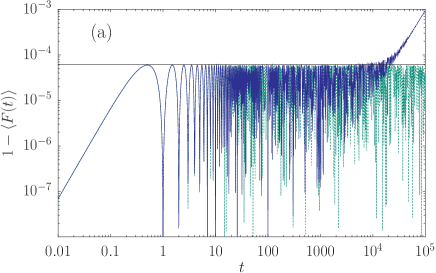
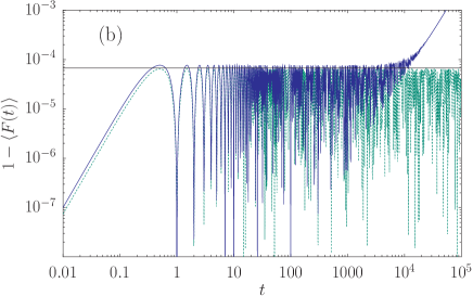
Figure 1: Comparison between the ensemble-averaged fidelity given by Eq. (16) (green/dashed curve) and numerical simulations (continuous/blue curve) for (a) $\beta=2$ and (b) $\beta=1$. In this case $k=2$, $\lambda=10^{-6}$, $n=1024$, $\epsilon_{1}=0.7618036$ and $\epsilon_{2}=0.9299698$. Notice that the agreement extends to times beyond $10^{3}t_{H}$. The horizontal lines display the value of the fidelity freeze according to Eq. (17).

We consider a normalized random initial state $|\Psi_{0}\rangle$, and make the simplification $|A_{\mu}|^{2}\sim 1/N$. We carry up the time integrals and compute the square modulus retaining terms up to second order in $\lambda$. Then, the ensemble-averaged fidelity to second order in $\lambda$ is given by

$$\overline{F_{\beta,\lambda}^{(2)}(t)}=1-\frac{2w_{k}^{2}\lambda^{2}}{n+1}\sum_{\mu\neq\rho}{\cal G}^{(k)}_{\mu,\rho}\frac{1-\cos[2\pi(\mu-\rho)t]}{[2\pi(\mu-\rho)]^{2}}+{\cal O}(\lambda^{4}).$$ (16)

Equation (16) is the main result in this paper. In Fig. 1 we show the comparison of the ensemble-averaged fidelity predicted by Eq. (16) with numerical calculations, both for $\beta=1$ and $\beta=2$. The results show excellent agreement even up to rather large values of $t$, when the fourth-order contributions in $\lambda$ eventually dominate and destroy the freeze of the fidelity. Notice that the agreement also holds for $\beta=1$, in spite of the fact that Eq. (16) was obtained for $\beta=2$. This confirms a posteriori that for $\beta=1$ the corrections to (14) are a factor $1/(n+1)$ smaller as assumed, and can be neglected in leading order in the boson number. The fact that Eq. (16) is not a perturbative expansion in time explains the good agreement for large values of $t$, which holds as $\lambda$ is small enough. In addition, for small times the results confirm the usual quadratic decay of the fidelity, namely, $1-\overline{F_{\beta,\lambda}^{(2)}(t)}\propto t^{2}+{\cal O}(t^{4})$. Fig. 2 displays the dependence of the ensemble-averaged fidelity with respect to $\lambda$ or $n$.

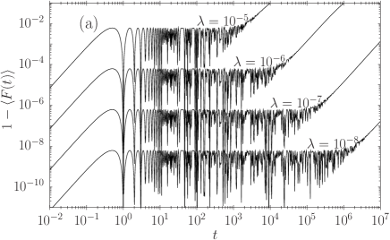
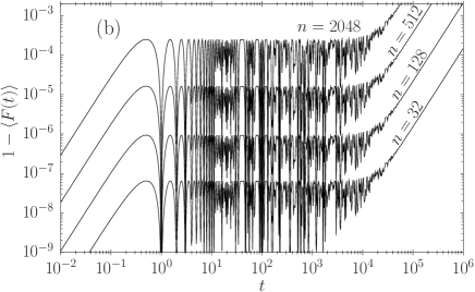
Figure 2: Ensemble-averaged fidelity decay for various values of (a) the perturbation strength $\lambda$, and (b) the number of particles $n$. Note that the time at which the fidelity freeze ends and decay sets back, $t_{e}$, is independent of $n$.

More interesting and far reaching is the fact that fidelity, up to second order in $\lambda$ is a Fourier cosine-series in $t$. The basic periodicity is precisely the Heisenberg time $t_{H}=1$, since the minimum difference in the occupation numbers for the states $|\mu\rangle$ and $|\rho\rangle$ in one of the single-particle states is precisely 1. Indeed, the double sum over the basis states excludes the case $\mu=\rho$, since for $\mu=\rho$ we have set ${\cal G}^{(k)}_{\mu,\mu}=0$ before the time-integration is carried up. This emphasizes the fact that the Fourier coefficients in Eq. (16) are related to the off-diagonal residual interaction. Moreover, we observe that, in units of the $t_{H}$, at integer values of time the time-dependent term of (16) vanishes identically, and therefore revival of $|\Psi_{0}\rangle$ are observed, as illustrated in  Fig. 1. These revivals are not a full recovery of $|\Psi_{0}\rangle$ though, since there may be corrections of higher order in $\lambda$, and Eq. (16) has been averaged over the ensemble. We emphasize that the periodicity $T_{f}=t_{H}$ of the revivals of the ensemble-averaged fidelity for the bosonic embedded ensembles follows from the fact that $\epsilon_{1}\neq\epsilon_{2}$, which is responsible for the complex exponential factor of Eq. (15).

Equation (16) permits to obtain an estimate of the freeze of the fidelity, which we denote by $F_{\rm freeze}$. Considering the minimum value for the fidelity when (16) is valid, that is, when the periodic revivals are observed because of the freeze of the fidelity, we have

$$F_{\rm freeze}=1-\frac{(w_{k}\lambda)^{2}}{\pi^{2}(n+1)}\sum_{\mu\neq\rho}\frac{{\cal G}^{(k)}_{\mu,\rho}}{(\mu-\rho)^{2}}.$$ (17)

Equation (17) predicts that $F_{\rm freeze}$ scales as $\lambda^{2}$. The scaling with respect to the number of particles is more involved since $w_{k}$ and the coefficients ${\cal G}_{\mu,\rho}^{(k)}$ depend on $n$. Using Stirling’s formula we obtain $w_{k}^{2}\sim n^{2-2k}$ and ${\cal G}_{\mu,\rho}^{(k)}\sim n^{2k}$, which yield the scaling $\sim n^{2}$, where we took into account that the sum over the many-body states cancels the normalization factor of the random initial state $|\Psi_{0}\rangle$. These scaling laws are confirmed numerically as illustrated in Fig. 3. At this point we note that the time $t_{e}$ during which the freeze of the fidelity lasts scales as $t_{e}\sim\lambda^{2}$ and is essentially independent of $n$; cf. Figs. 2 and 3.

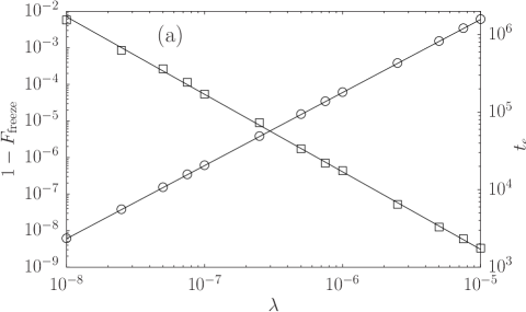
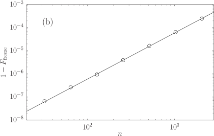
Figure 3: (a) Dependence of the freeze of the fidelity (circles) upon $\lambda$, which confirms that $1-F_{\rm freeze}\propto\lambda^{2}$. The right vertical scale indicates the time of duration of the freeze of the fidelity (data in squares) which shows the scaling $t_{e}\propto 1/n$. (b) Dependence of $F_{\rm freeze}$ on $n$ confirming the scaling $1-F_{\rm freeze}\propto n^{2}$.

IV Periodic fractional revivals and $k$-body interactions

As discussed above, Eq. (16) predicts periodic time-revivals of fixed period $T_{f}=t_{H}=1$, independently of the rank $k$ of the residual interaction. This is a consequence of the fact that the residual $k$-body interaction so far considered, contains terms which involve moving $1,2,\dots,k$ particles, from one of the single-particle levels to the other. That is, the many-body states coupled through the perturbation $\hat{V}_{k}(\beta)$ may differ at least in the occupation of one particle, and at most in the occupation of $k$. These differences are precisely the factors $\mu-\rho$ that appear in the Fourier expansion in Eq. (16), which denote the difference of number of particles in a given single-particle level. Clearly, the minimum difference fixes the periodicity of the Fourier cosine series.

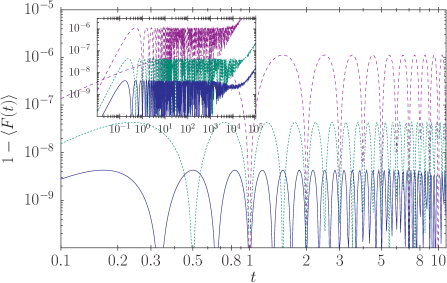
Figure 4: Ensemble-averaged fidelity decay for the residual interaction $\hat{\cal K}_{k}$ in Eq. (18) for $k=2$ (green/dotted curve) and $k=3$ (blue/continuous curve), illustrating the fractional periodic revivals. These correspond to $T_{f}=1/2$ and $T_{f}=1/3$, respectively. The magenta/dashed curve displays the result when all off-diagonal elements for $k=3$ of (1) are considered.

This explanation opens the following interesting possibility. By selecting the actual perturbing terms within the $k$-body residual interaction, we can actually tune the observed periodicity of the revivals during the fidelity freeze, in particular, making it different from Heisenberg time $T_{f}=1$. Indeed, we can fix the perturbation such that the only terms present move exactly $k$ particles from one single-particle level to the other one. That is, we restrict the general $k$-body Hamiltonian (1) such that the off-diagonal terms are

$$\hat{\cal K}_{k}=v_{k,0}(\hat{a}_{1}^{\dagger})^{k}(\hat{a}_{2})^{k}+v_{0,k}(\hat{a}_{2}^{\dagger})^{k}(\hat{a}_{1})^{k},$$ (18)

with $v_{k,0}=(v_{0,k})^{*}$ to ensure hermitecity. This choice of the residual interaction implies that the Fourier coefficients vanish unless $|\mu-\rho|=k$, that is, when the states $|\mu\rangle$ and $|\rho\rangle$ precisely differ in the occupation of $k$ particles with respect to one mode. In this case, the argument of the cosine function in Eq. (16) is $2\pi kt$, which implies that the periodicity of the revivals during the freeze of the fidelity becomes $T_{f}=1/k$ in units of the Heisenberg time. Apart from the fact that this periodicity differs from $1$, the important aspect is that the periodicity of the revivals during the freeze of the fidelity provides a direct measure of the rank of the interaction $k$ of the residual perturbation $\hat{\cal K}_{k}$. These are the fractional periodic revivals.

This prediction is illustrated in Fig. 4, where we plot the ensemble-averaged fidelity for an interaction of the form (18) for $k=2$ and $k=3$, and for comparison a case including all off-diagonal contributions of $\hat{H}_{k}$ in Eq. (1). The results clearly show $T_{f}=1/2$, $T_{f}=1/3$ for the first two cases, reflecting the value of the corresponding $k$-body interactions, and $T_{f}=1$, as expected from Eq. (16).

V Conclusions

In this paper, we have studied analytically and numerically the fidelity decay in the $k$-body embedded ensemble of random matrices for bosons distributed in two single-particle levels. We defined fidelity in terms of a reference Hamiltonian, which is assumed to be in diagonal form, and a perturbed Hamiltonian which in addition includes a purely off-diagonal residual $k$-body interaction. This situation mimics the typical set-up in mean-field calculations, but appears also in other interesting physical cases, such as time-reversal symmetry-breaking. This set-up fulfills the conditions to observe the freeze of the fidelity ProsenZnid2003 ; GKPSSZ2006 , thus allowing for longer control of the system.

We calculated the ensemble-averaged fidelity within the linear response theory up to second-order in the perturbation parameter, which is a Fourier series whose basic periodicity is equal to the Heisenberg time $t_{H}$. The analytical predictions are in good correspondence with the direct numerical results, confirming the presence of the freeze for the ensemble-averaged fidelity as well as the relevant scalings with respect to the strength of the perturbation and the number of particles of the system. The oscillatory part of this Fourier series cancels at integer times of $t_{H}$, thus manifesting the periodicity of the revivals. Selecting the off-diagonal terms of the $k$-body residual interaction, in order that the actual perturbation couples only many-body states differing exactly by $k$ particles in the occupation number of either single-particle level, we showed that the periodicity of the revivals becomes $1/k$ in units of the Heisenberg time. Therefore, the periodicity of the revivals of the ensemble-average fidelity during freeze may be used as a direct measure to detect the rank $k$ of the perturbing interaction. This aspect may be interesting in the context of current efforts that address effects related to three–body interactions Buechler2007 ; Johnson2009 which are responsible, for instance, for atomic losses in ultra-cold bosonic gases.

- (1) T. Gorin, T. Prosen, T.H. Seligman, and M. Žnidarič, Phys. Rep 435, 33 (2006).
- (2) T. Prosen and M. Žnidarič, New J. Phys. 5, 109 (2003); T. Prosen and M. Žnidarič, Phys. Rev. Lett. 94, 044101 (2005).
- (3) I. Pižorn, T. Prosen and T.H. Seligman, Phys. Rev. B 76 035122 (2007).
- (4) O.I. Lobkis and R.L. Weaver, Phys. Rev. Lett. 90, 254302 (2003).
- (5) T. Gorin, T.H. Seligman and R.L. Weaver, Phys. Rev. E 73, 015202(R) (2006).
- (6) L. Benet, C. Jung and F. Leyvraz, J. Phys. A: Math. Gen. 36, L217 (2003).
- (7) B.P. Anderson, M.A. Kasevich, Science 282, 1686 (1998).
- (8) M. Albiez, R. Gati, J. Fölling, S. Hunsmann, M. Cristiani, and M. K. Oberthaler, Phys. Rev. Lett. 95, 010402 (2005).
- (9) O. Morsch and M. Oberthaler, Rev. Mod. Phys. 78, 179 (2006).
- (10) R. Gati, M.K. Oberthaler, J. Phys. B: At. Mol. Opt. Phys. 40, R61 (2007).
- (11) J.B. French and S.S.M. Wong, Phys. Lett. B 33, 449 (1970); J.B. French and S.S.M. Wong, Phys. Lett. B 35, 5 (1971).
- (12) O. Bohigas and J. Flores, Phys. Lett. B 34, 261 (1971), O. Bohigas and J. Flores, Phys. Lett. B 35 383 (1971).
- (13) K.K. Mon and J.B. French, Ann. Phys. (N.Y.) 95, 90 (1975).
- (14) V.K.B. Kota and V. Potbhare, Phys. Rev. C 21, 2637 (1980).
- (15) V.R. Manfredi, Lett. Nuovo Cimento 40, 135 (1984).
- (16) T. Asaga, L. Benet, T. Rupp and H.A. Weidenmüller, Eurphys. Lett. 56, 340 (2001); ibid, Ann. Phys. (N.Y.) 298, 229 (2002).
- (17) I. Pižorn, T. Prosen, S. Mossmann and T.H Seligman, New J. Phys. 10, 023020 (2008).
- (18) V.K.B. Kota, Phys. Rep. 347, 223 (2001).
- (19) L. Benet and H.A. Weidenmüller, J. Phys. A: Math. Gen. 36, 3569 (2003).
- (20) L. Benet, S. Hernández-Quiroz and T.H. Seligman, AIP Conf. Proc. 1323, 6 (2010).
- (21) L. Benet, F. Leyvraz and T.H. Seligman, Phys. Rev. E 68, 045201(R) (2003).
- (22) S. Hernández-Quiroz and L. Benet, Phys. Rev. E 81, 036218 (2010).
- (23) T. Guhr, A. Mueller-Gröling and H. A. Weidenmüller, Phys. Rep. 299, 189 (1998).
- (24) A. I. Shnirelman, Usp. Mat. Nauk 30, 265 (1975); A. I. Shnirelman, addendum in V. F. Lazutkin, KAM Theory and Semiclassical Approximations to Eigenfunctions (Springer, Berlin, 1993).
- (25) T. Gorin, et al., Phys. Rev. Lett. 96, 244105 (2006).
- (26) T. Prosen, Phys. Rev. E 65, 036208 (2002); T. Prosen and M. Žnidarič, J. Phys A: Math Gen 35, 1455 (2002).
- (27) H.P. Büchler, A. Micheli and P. Zoller, Nature Physics 3 726 (2007).
- (28) P. R. Johnson, E. Tiesinga, J. V. Porto and C. J. Williams, New Journal of Physics 11, 093022 (2009), and references therein.