SDO Observations of Magnetic Reconnection at Coronal Hole Boundaries

Abstract

With the observations from the Atmospheric Imaging Assembly (AIA) and the Helioseismic and Magnetic Imager (HMI) aboard the Solar Dynamics Observatory, we investigate the coronal hole boundaries (CHBs) of an equatorial extension of polar coronal hole. At the CHBs, lots of extreme-ultraviolet (EUV) jets, which appear to be the signatures of magnetic reconnection, are observed in the 193 Å images, and some jets occur repetitively at the same sites. The evolution of the jets is associated with the emergence and cancelation of magnetic fields. We notice that both the east and the west CHBs shift westward, and the shift velocities are close to the velocities of rigid rotation compared with those of the photospheric differential rotation. This indicates that magnetic reconnection at CHBs results in the evolution of CHBs and maintains the rigid rotation of coronal holes.

1 Introduction

Coronal holes (CHs) are dark areas which can be observed at both the low latitudes and the polar regions of the Sun using X-ray and extreme-ultraviolet (EUV) lines (Chiuderi Drago et al. 1999). The magnetic fields within a CH region are dominated by one polarity, and thus the field lines in the upper atmosphere are open to the interplanetary region, generating high-speed solar winds that can lead to geomagnetic storms (Bohlin 1977; Krieger & Timothy 1973; Tu et al. 2005). Many basic characters of CHs and their relationship with magnetic fields have been studied (Wiegelmann & Solanki 2004; Meunier 2005; Zhang et al. 2006, 2007; Yang et al. 2009a, b). Using observations from the Solar Ultraviolet Measurements of Emitted Radiation (SUMER) instrument onboard the Solar and Heliospheric Observatory (SOHO), blue shifts indicating plasma flows within CHs are intensively investigated (Hassler et al. 1999; Peter & Judge 1999; Xia et al. 2004; Aiouaz et al. 2005; McIntosh et al. 2011). Recently, Hinode (Kosugi et al. 2007) observations display that CHs are nonpotential, e.g., in some strong magnetic field regions within CHs, the current densities are as large as those in flare productive active regions (Yang et al. 2011).

CHs can be classified into two types according to their locations: polar CHs and mid-latitude ones (Insley et al. 1995; Wang et al. 1996). The mid-latitude CHs can be “isolated” or connected with polar CHs called equatorial extensions of polar CHs (EECHs) (Insley et al. 1995). Observations reveal that EECHs rotate quasi-rigidly although the photosphere rotates differentially (Timothy et al. 1975; Insley et al. 1995; Wang et al. 1996). CH boundaries (CHBs) separate two kinds of areas with different configurations: CHs with open magnetic fields and surrounding quiet Sun with closed magnetic fields. Due to the fact that EECHs rotate rigidly while the underlying photospheric fields differentially, magnetic reconnection is necessary to happen at CHBs to maintain the rigid rotation of the CHs (Wang & Sheeley 1994; Fisk, et al. 1999).

Kahler & Moses (1990) studied an EECH in Skylab X-ray images and noticed that X-ray bright points at CHBs play an important role in the CH expansion and contraction. Kahler & Hudson (2002) studied three EECHs observed by the Yohkoh Soft X-ray telescope, however, they found no significant effect for bright points on CHB evolution. Using EUV images from the Transition Region and Coronal Explorer (TRACE) and the SOHO, Madjarska & Wiegelmann (2009) investigated the evolution of CHBs at small scales. They found that small-scale magnetic loops (appeared as bright points) play an important role in CHB evolution but did not find signature for a major energy release during the evolution of loops. Kahler et al. (2010) also focused on the changes of CHBs. But in their study, no example of the energetic jet was reported in EUV images. According to previous studies, jets are transient plasma ejections which are believed to result from magnetic reconnection (Shibata et al. 1992, 1994; Yakoyama & Shibata 1995). More recently, Subramanian et al. (2010) explored CHB evolution with the images from XRT on board Hinode. They observed some jet-like events at CHB regions and those ejections appeared to be triggered by magnetic reconnection.

The aim of this study is to examine if there exist some signatures (e.g., jets) of magnetic reconnection at CHBs in the EUV images from the Solar Dynamics Observatory (SDO; Schwer et al. 2002). In Sections 2 and 3, the observations and results are presented respectively. The conclusions and discussion are given in Section 4.

2 Observations and Data Analysis

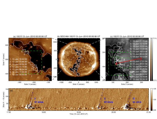
Figure 1: SDO$/$AIA 193 Å full-disk image (panel b) obtained on 13 June 2010 showing an EECH, and sub-images (panels a and c) with sharp CHBs. Panel d is running ratio space-time plot along slit “A—B” (red line in panel c). The contours represent CHBs. The white rectangles in panels a and c show jets occurring at the CHBs at different times. The dotted rectangles (left and right) in panel c outline the FOVs of Figures 2 and 3, respectively, and two dashed squares in panels a and c the FOVs of Figures 4 and 5, respectively.

The CH studied here is an EECH extended from the south pole to N41$\arcdeg$ in the middle of 2010 June (see Figure 1b). The data used here were obtained by the Atmospheric Imaging Assembly (AIA; Title et al. 2006) and the Helioseismic and Magnetic Imager (HMI; Schou et al. 2011) aboard the SDO from June 10 to June 15. The AIA takes full-disk images in 10 wavelengths with pixel size of 0$\arcsec$.6 and we use the 193 Å data at Level 1.5 with 12 s cadence to study the CH. We also adopt the full-disk line-of-sight magnetograms with 45 s cadence obtained by the HMI at 6173 Å with a spatial sampling of 0$\arcsec$.5 pixel^-1. The 193 channel contains lines from both Fe XII and Fe XXIV, and the corresponding temperatures are 1.5 MK and 20 MK, respectively. Among 10 wavelengths of AIA, 193 Å mainly reveals information of corona, 304 Å and 171 Å are mainly formed in chromosphere and transition region, while other lines are sensitive in response to the active region or flaring corona. Since CHs are low density and low temperature regions in the corona, so we choose 193 Å as the most appropriate one to study CHs. We can find that CHs are clearly visible in 193 Å images.

The AIA images and HMI magnetograms are differentially rotated to a reference time (2010 June 13 00:00:06 UT) when the CH was mainly located at the central meridian. In this study, the AIA images are displayed on logarithmic scale and the HMI magnetograms are averaged every three frames. The CHBs are determined as the regions with intensities 1.5 times the average intensity of the darkest region inside the CH, the same as the method that Madjarska & Wiegelmann (2009) used. We define the CHB regions as $\pm$ 15$\arcsec$ on both sides of the CHBs, as Subramanian et al. (2010) did in their study.

3 Results

Some parts of the CHB are diffuse, so we select two parts (Figures 1a and 1c, also outlined by two squares in Figure 1b) which are sharp enough to be defined well. In the early morning of 2010 June 13, the main body of the CH was mainly at the central meridian. To avoid projection effects (Kahler & Hudson 2002; Kahler et al. 2010), we use only the limbward CHB observations, i.e., the east CHB (ECHB) on June 12 (Figure 1a) and the west CHB (WCHB) on June 13 (Figure 1c).

3.1 Signatures of Magnetic Reconnection at the CHBs

The background of Figure 1a is an AIA 193 Å image at 00:00:06 UT on 2010 June 13. The sub-regions outlined by white rectangles display the jets occurring at different times on June 12, and the time of each jet is also listed in the Figure. In a one-day period, seven sites with bright jets are observed at the ECHB, as presented in Figure 1a. At the WCHB, more jets appeared (Figure 1c). On June 13, we find fifteen sites at the WCHB where obvious jets occurred. Here, we identify the jets by eye according to their appearance and evolution in 193 Å movies, instead of with automatic techniques. The automatic detection methods introduced in the newly published paper of Martens et al. (2011) will be helpful for us to investigate the jets at CHBs in future.

Some jets occurred repetitively at the same sites (e.g., in rectangle “8” in Figure 1c). Along slit “A—B”, we obtain the image profile by averaging five pixels in the running ratio images in the direction perpendicular to “A—B”. Then we make the running ratio space-time plot of such profiles over time from 17:00 UT to 21:00 UT, as shown in Figure 1d. During this period, three obvious jets are observed, as labeled with “i”, “ii”, and “iii,” and their lifetimes are about 12 minutes. The projection velocities of these three jets are 61 km s^-1, 61 km s^-1, and 54 km s^-1, respectively.

3.2 Evolution of the Jets at the CHBs

The sequence of 193 Å images in Figure 2 (from a to d) display the evolution of two jets located at the WCHB (also see rectangle “5” in Figure 1c). The underlying magnetic fields are presented in Figures 2e–h. At 16:44:03 UT, a cluster of magnetic elements with mixed polarities (denoted by arrow “3”) emerged at the CHB, and the negative flux, opposite to the surrounding polarities, became larger at 18:44:03 UT. During this process, bright point in the 193 Å images was observed at the location of magnetic emergence (indicated by arrow “1”). The newly emerged negative elements moved toward the surrounding positive ones and canceled with them (panels g–h). Above the cancelation region, two jets (denoted by arrows “2”) occurred in the corona (panels b–c) and then decayed (panel d).

Figure 3 presents the evolution process of another jet. At 20:09:06 UT, the area outlined by the square was a CHB region without obvious coronal activity (Figure 3a). Several minutes later, a jet appeared (denoted by arrow “1”). At 20:20:18, the jet had become more violent (Figure 2c). The decay of the jet is displayed in Figures 3d–e, and at 20:59:18 UT (Figure 3f), the jet disappeared. Correspondly, there are some changes in the underlying magnetic fields (Figures 3g–i). At 20:08:03 UT, before the occurrence of the jet, there existed lots of magnetic elements with opposite polarities (denoted by arrows labeled “2”). During the jet evolution, the negative elements canceled with the positive ones (Figure 3h). At 21:29:03 UT, the total magnetic flux decreased obviously and only several minor elements were remained (Figure 3i).

3.3 Shifts of the CHBs

In order to analyze the shifts of the CHBs, the derotated sub-images outlined by two dashed squares in Figure 1 are mapped into heliographic coordinates and used in Figures 4 and 5.

The FOV of Figure 4 covers a part of sharp ECHB. Panels a–d show the changes of ECHB on June 12. We can find some jets occurred at the ECHB (denoted by arrows “1” and “2”; see also Figure 1a). To examine the shift of ECHB, we make three space-time plots along three slits (“A—B”, “C—D”, and “E—F” in Figure 4b) in the latitudinal direction, and display them in Figures 4e–g, respectively. In the plots, each profile is obtained by averaging five pixels in 193 Å images in the direction perpendicular to the slits. The shift velocity of the ECHB at each site is derived by a linear fitting. We find that the shift velocities at three sites are 0$\arcdeg$.755 $\pm$ 0$\arcdeg$.008 day^-1, 0$\arcdeg$.619 $\pm$ 0$\arcdeg$.004 day^-1, and 0$\arcdeg$.369 $\pm$ 0$\arcdeg$.003 day^-1, respectively. The feature denoted by arrow “3” in panel f represents a jet. However, we find no obvious jet in panels e and g.

We also study a sharp section of WCHB, which is presented in Figure 5. Figures 5a–d exhibit the WCHB at different stages on June 13. Arrows “1” and “2” denote two jets appearing at the WCHB and more jets can be found in Figure 1c. Similarly as we deal with the ECHB, space-time plots along the slits “A—B”, “C—D”, “E—F” (see Figure 5b) are obtained and given in Figures 5e–g. In the three plots, we obtain the fitted velocities: 0$\arcdeg$.789 $\pm$ 0$\arcdeg$.009 day^-1, 1$\arcdeg$.015 $\pm$ 0$\arcdeg$.005 day^-1, and 0$\arcdeg$.949 $\pm$ 0$\arcdeg$.007 day^-1, respectively. The bright features indicated by arrows “3”–“5” are jets at the WCHB.

4 Conclusions and Discussion

By employing the observations from the AIA and HMI on board the SDO, we investigate the CHBs of an EECH. At the CHBs, a lot of jets are found in the 193 Å images, and some jets occurred repetitively at the same sites. The evolution of the jets is associated with emergence and cancelation of the underlying magnetic fields. We notice that both the ECHB and the WCHB shift westward, and the shift velocities are close to the velocities of rigid rotation compared with those of the photospheric rotation.

Subramanian et al. (2010) observed X-ray jets at CHBs with Hinode XRT data and they thought that those ejections appeared to be triggered by magnetic reconnection. In this study, we have observed many bright jets at both the ECHB and the WCHB in the EUV line images from the SDO. We think that these EUV jets are the observational signatures of magnetic reconnection at CHBs. In this study, more jets are observed at the WCHB than at the ECHB. It seems that this phenomenon is consistent with the concept of the E—W asymmetry in the CHB reconnection as discussed in Kahler et al. (2010).

We notice that some jets occurred repetitively at the same sites (see Figure 1d). The recurrence of the jets at CHBs is similar to the events in CHs, quiet regions, and active regions. Wang et al. (1997) and Chae et al. (1998, 1999) studied the disk and limb jets in quiet and active regions and found that the jets occurred repeatedly at the same sites. Repetitive occurrence of jets in CHs is also presented in the study of Subramanian et al. (2010). They reported that many bright points produced several jet-like events with no periodicity.

The average projection velocity of the jets in this study is about 60 km s^-1. It is difficult to know the real velocities of the jets from the projection velocities in this study. But if we assume the jets are locally vertical and combine with their heliocentric angle of almost 30$\arcdeg$, the real velocities should be around 120 km s^-1, about 2 times the projection velocities. Cirtain et al. (2007) studied four jets in detail and found there are two velocity components for each jet. one component is slow velocity of $\sim$200 km s^-1, close to the sound speed, and the other one observed at the start of each event is roughly $\sim$800 km s^-1, close to the Alfvén speed. They considered them as two kinds of outflows during the post-magnetic reconnection phase of a jet. Savcheva et al. (2007) statistically studied a large sample of jets and found that the outward velocity shows a peaked distribution with a maximum at 160 km s^-1. The estimated real velocity (120 km s^-1) in our study is generally consistent with those of Cirtain et al. (2007; 200 km s^-1) and many other former studies (Shibata et al. 1992; Shimojo et al. 1996; Savcheva et al. 2007). So we think that the jets with low velocities in our study are also resulted from magnetic reconnection, since they have been considered as one kind of outflows during the post-magnetic reconnection phase (Cirtain et al. 2007), though they might be directly driven by magnetosonic shock waves. In this study, we do not derive high velocity of about 800 km s^-1. Savcheva et al. (2007) introduced a “brightness contour method” which can detect high velocities of about 600–1000 km s^-1, but the error bars on the high velocities are usually very large. However, this method can be considered to use to study jets in detail in future.

In the studies of Madjarska & Wiegelmann (2009) and Subramanian et al. (2010), no photospheric magnetogram is used. So the evolution of magnetic fields associated with the bright points and jets at CHBs is not clear. With the HMI observations, we are able to know the evolution process of the magnetic fields underlying the coronal jets at the CHBs. When the jets occurred, magnetic emergence and cancelation were observed, as shown in Figures 2 and 3.

Since the AIA images are differentially rotated to a reference time, the CHBs should shift westward if the CH rotates rigidly and should keep stable without shift if the CH rotates differentially with the photosphere. After calculation, we know that, if the CH rotates rigidly, the shift velocity of the ECHB shown in Figure 4 should be 0$\arcdeg$.669 day^-1 and that of the WCHB in Figure 5 should be 0$\arcdeg$.490 day^-1. Actually, we obtain that the mean velocities of the ECHB and the WCHB are 0$\arcdeg$.581 day^-1 and 0$\arcdeg$.918 day^-1, respectively. The observed shift velocities are close to those required to maintain the rigid rotation compared with those of the photospheric differential rotation. It provides us exact evidences of the concept that magnetic reconnection at CHBs results in the evolution of CHBs and maintains the rigid rotation of CHs. The shift velocity of the WCHB is higher than the rigid rotation requires, which may be caused by the intensive magnetic reconnection indicated by more jets at the WCHB during this period.

However, not all the CHB shifts are accompanied by obvious signatures (such as jets) of magnetic reconnection, as revealed in Figures 4e and g. We think this may be caused by the concept that the reconnection at CHBs occurs just below the potential-field source surface (PFSS) (Wang & Sheeley 1994; Fisk 2005; Schwadron et al. 2005; Wang et al. 2007). This explanation is also adopted in the study of Kahler et al. (2010). They argued that gradual reconnection occurs at high altitudes, so they did not find jets and flare-like events in the EUV images. In our opinion, short period (about seven hours) and low cadence (4.4 min) observations could lead to the absence of jets in the EUV images. In addition, another possible reason is that magnetic reconnection at some sites is too weak to be observed. Based on the results, we think magnetic reconnection at CHBs can take place in the low corona indicated by the jets in 193 Å images, also in the high layer just below the PFSS as mentioned above.

In this Letter, we present the general appearance of the signatures, i.e. the jets in 193 Å images, of magnetic reconnection at the CHBs. But there are still lots of questions. Does the reconnection occur between open field lines in the CH and closed loops in the surrounding quiet Sun regions? Where does the reconnection take place and in which layer are the jets accelerated? Is it in corona or the lower regions? Is it possible that the formation of jets is caused by reconnection between low lying loops in the CH which can not extend in to the corona and significantly high coronal loops in the quiet Sun? As pointed out by the referee, observations in the other cooler wavelengths formed in chromosphere and transition region might help to get more insights regarding reconnection at CHBs, which can be taken into consideration in our next study.

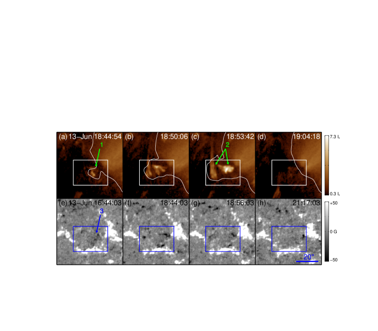
Figure 2: Sequence of AIA 193 Å images (upper panels) displaying the evolution of two jets, and HMI longitudinal magnetograms (lower panels) showing the underlying magnetic fields. The curves delineate CHBs and the rectangles outline the area within which magnetic emergence and cancelation took place. Arrows “1”, “2”, and “3” denote the bright point, jets, and emerging magnetic flux, respectively.

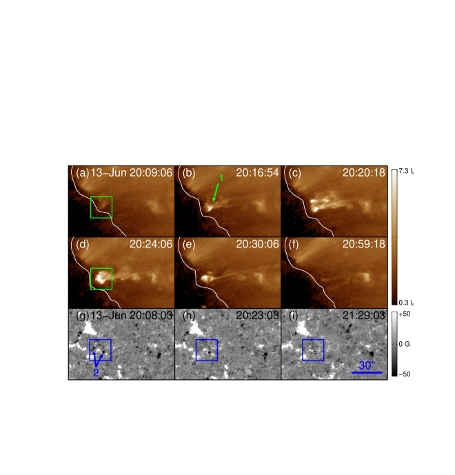
Figure 3: AIA images (panels a–f) and HMI magnetograms (panels g–i) exhibiting a signature of magnetic reconnection. The curves delineate CHBs and the squares outline the area where magnetic cancelation occurred. Arrows “1” and “2” indicate the jet and negative magnetic elements, respectively.

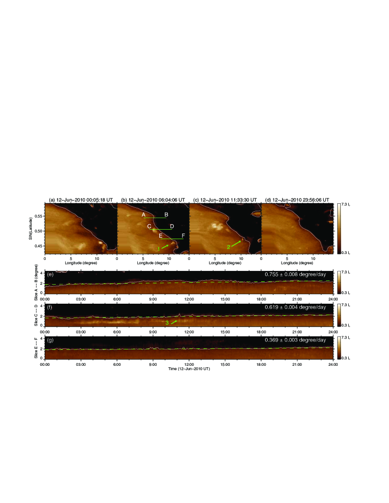
Figure 4: ECHB shift revealed in 193 Å images mapped into heliographic coordinates (panels a–d) and space-time plots (panels e–g) along slits “A—B”, “C—D”, and “E—F” (see panel b), respectively. The curves delineate CHBs and the arrows denote jets. The dashed lines are linear fits to the CHBs.

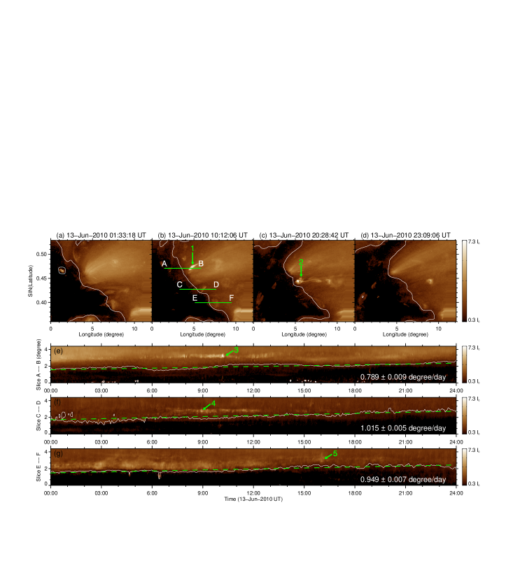
Figure 5: Similar to Figure 4 but for the WCHB.

References

- (1) Aiouaz, T., Peter, H., & Lemaire, P. 2005, A&A, 435, 713
- (2) Bohlin, J. D. 1977, Sol. Phys., 51, 377
- (3) Chae, J., et al. 1998, ApJ, 504, 123
- (4) Chae, J., Qiu, J., Wang, H. M., & Goode, P. R. 1999, ApJ, 513, 75
- (5) Chiuderi Drago, F., Landi, E., Fludra, A., & Kerdraon, A. 1999, A&A, 348, 261
- (6) Cirtain, J. W., Golub, L., Lundquist, L., et al. 2007, Science, 318, 1580
- (7) Fisk, L. A. 2005, ApJ, 626, 563
- (8) Fisk, L. A., Zurbuchen, T. H., & Schwadron, N. A. 1999, ApJ, 521, 868
- (9) Hassler, D. M., et al. 1999, Science, 283, 810
- (10) Insley, J. E., Moore, V., & Harrison, R. A. 1995, Sol. Phys., 160, 1
- (11) Kahler, S. W., & Hudson, H. S. 2002, ApJ, 574, 467
- (12) Kahler, S. W., Jibben, P., & DeLuca, E. E. 2010, Sol. Phys., 262, 135
- (13) Kahler, S. W., & Moses, D. 1990, ApJ, 362, 728
- (14) Kosugi, T., et al. 2007, Sol. Phys., 243, 3
- (15) Krieger, A. S., Timothy, A. F., & Roelof, E. C. 1973, Sol. Phys., 29, 505
- (16) Madjarska, M. S., & Wiegelmann, T. 2009, A&A, 503, 991
- (17) Martens, P. C. H., Attrill, G. D. R., Davey, A. R., et al. 2011, Sol. Phys., DOI:10.1007/s11207-010-9697-y
- (18) McIntosh, S. W., Leamon, R., J., & De Pontieu, B. 2011, ApJ, 727, 7
- (19) Meunier, N. 2005, A&A, 443, 309
- (20) Peter, H., & Judge, P. G. 1999, ApJ, 522, 1148
- (21) Savcheva, A., Cirtain, J., DeLuca, E. E., et al. 2007, PASJ, 59, S771
- (22) Schwadron, N. A., et al. 2005, J. Geophys. Res., 110, A04104
- (23) Schwer, K., Lilly, R. B., Thompson, B. J., & Brewer, D. A. 2002, AGU Fall Meeting Abstracts, C1
- (24) Schou, J., Scherrer, P. H., Bush, R. I., Wachter, R., Couvidat, S., et al. 2011, Sol. Phys., in preparation.
- (25) Shibata, K., Ishido, Y., Acton, L.W., et al. 1992, PASJ, 44, L173
- (26) Shibata, K., Nitta, N., Matsumoto, R., et al. 1994, in X-ray solar physics from Yohkoh, ed. Y. Uchida, T. Watanabe, K. Shibata, & H. S. Hudson, 29
- (27) Shimojo, M., Hashimoto, S., Shibata, K., et al. 1996, PASJ, 48, 123
- (28) Subramanian, S., Madjarska, M. S., & Doyle, J. G. 2010, A&A, 516, 50
- (29) Timothy, A. F., Krieger, A. S., & Vaiana, G. S. 1975, Sol. Phys., 42, 135
- (30) Title, A. M., Hoeksema, J. T., Schrijver, C. J., & The Aia Team 2006, COSPAR Plenary Meeting, 36th COSPAR Scientific Assembly, 2600
- (31) Tu, C. Y., Zhou, C., Marsch, E., et al. 2005, Science, 308, 519
- (32) Wang, H. M., Johannesson, A., Stage, M., Lee, C., & Zirin, H. 1998, Sol. Phys., 178, 55
- (33) Wang, Y. M., Biersteker, J. B., Sheeley, N. R., Koutchmy, S., Mouette, J., & Druckm ller, M. 2007, ApJ, 660, 882
- (34) Wang, Y. M., Hawley, S. H., & Sheeley, N. R. 1996, Science, 271, 464
- (35) Wang, Y. M., & Sheeley, N. R. 1994, ApJ, 430, 399
- (36) Wiegelmann, T., & Solanki, S. K. 2004, Sol. Phys., 225, 227
- (37) Xia, L. D., Marsch, E., & Wilhelm, K. 2004, A&A, 424, 1025
- (38) Yang, S. H., Zhang, J., & Borrero, J. M. 2009a, ApJ, 703, 1012
- (39) Yang, S. H., Zhang, J., Jin, C. L., et al. 2009b, A&A, 501, 745
- (40) Yang, S. H., Zhang, J., Li, T., & Ding, M. D. 2011, ApJ, 726, 49
- (41) Yokoyama, Y., & Shibata, K. 1995, Nature, 375, 42
- (42) Zhang, J., Ma, J., & Wang, H. M. 2006, ApJ, 649, 464
- (43) Zhang, J., Zhou, G. P., Wang, J. X., & Wang, H. M. 2007, ApJ, 655, L113