Spin-aligned neutron-proton pairs in $N=Z$ nuclei

Abstract

A study is carried out of the role of the aligned neutron-proton pair with angular momentum $J=9$ and isospin $T=0$ in the low-energy spectroscopy of the $N=Z$ nuclei ⁹⁶Cd, ⁹⁴Ag, and ⁹²Pd. Shell-model wave functions resulting from realistic interactions are analyzed in terms of a variety of two-nucleon pairs corresponding to different choices of their coupled angular momentum $J$ and isospin $T$. The analysis is performed exactly for four holes (⁹⁶Cd) and carried further for six and eight holes (⁹⁴Ag and ⁹²Pd) by means of a mapping to an appropriate version of the interacting boson model. The study allows the identification of the strengths and deficiencies of the aligned-pair approximation.

I Introduction

The study of nuclei with equal numbers of neutrons and protons ($N=Z$) is one of the declared goals of radioactive-ion-beam facilities, either in operation or under construction. Such nuclei are well known when $N$ and $Z$ are small but, as the atomic mass number $A=N+Z$ increases, they lie increasingly closer to the proton drip line and therefore become more difficult to study experimentally. Nevertheless, several phenomena of interest, such as the breaking of isospin symmetry or the emergence of new collective modes of excitation, are predicted to become more pronounced with increasing $A$, and this constitutes the main argument for undertaking the difficult studies of ever more heavier $N=Z$ nuclei.

Arguably, the goal of most interest in this quest is the uncovering of effects due to isoscalar ($T=0$) neutron-proton (n-p) pairing. In contrast to the usual isovector ($T=1$) pairing, where the orbital angular momenta and the spins of two nucleons are both antiparallel (i.e., $L=0$ and $S=0$), isoscalar pairing requires the spins of the nucleons to be parallel ($S=1$), resulting in a total angular momentum $J=1$. Collective correlation effects are predicted to occur as a result of isoscalar n-p pairing Warner06 but have resisted so far experimental confirmation because (i) the $jj$ coupling scheme which is applicable in all but the lightest nuclei disfavors the formation of isoscalar n-p pairs with $L=0$ Juillet00 , and (ii) the states associated with this collective mode are of low angular momentum $J$ and often hidden among high-$J$ isomeric states which hinders their experimental detection.

Currently, $N=Z$ experiments are approaching ¹⁰⁰Sn, involving studies of nuclei such as ⁹²Pd Cederwall10 where nucleons are dominantly confined to the $1g_{9/2}$ orbit. In the context of these experiments, Blomqvist recently proposed Blomqvist that a realistic description of shell-model wave functions can be obtained in terms of isoscalar n-p pairs which are completely aligned in angular momentum, that is, pairs with $J=9$. This proposal is attractive since it is well adapted to the $jj$ coupling scheme, valid in this mass region, and because it should encompass the description of high-$J$ isomeric states. Blomqvist’s idea is related to the so-called stretch scheme which was advocated a long time ago by Danos and Gillet Danos67 . In the stretch scheme, shell-model states are constructed from aligned n-p pairs, treated in a quasi-boson approximation which neglects antisymmetry between the nucleons in different pairs. The latter approximation is absent from Blomqvist’s approach.

In this paper we examine Blomqvist’s proposal for the $N=Z$ nuclei ⁹⁶Cd, ⁹⁴Ag, and ⁹²Pd. We consider several realistic two-body interactions for the $1g_{9/2}$ orbit and analyze the shell-model wave functions, obtained with these interactions, of the four-nucleon-hole system (⁹⁶Cd), in terms of a variety two-pair states. For the six- and eight-hole nuclei (⁹⁴Ag and ⁹²Pd) a direct shell-model analysis in terms of pair states is more difficult, and we prefer therefore to carry out an indirect check by means of a mapping to a corresponding boson model. In these cases our approach is intermediate between that of Blomqvist Blomqvist and of Danos and Gillet Danos67 . The boson mapping takes care of antisymmetry effects in an exact manner on the level of four nucleons but becomes approximate for more.

This paper is organized as follows. First, some necessary concepts and techniques are introduced: the formulas needed to carry out a shell-model calculation in a pair basis are given in Sect. II and two mapping techniques from an interacting fermion to an interacting boson model are reviewed in Sect. III. The results of our analysis of $N=Z$ nuclei are presented and discussed in Sect IV. The conclusions and outlook of this work are summarized in Sect. V.

II Four-particle matrix elements

This section summarizes the necessary ingredients to carry out calculations in an isospin formalism. The formulas given are valid for fermions as well as for bosons. Four-particle states are described by grouping the particles in two pairs. These two-pair states can be used, for example, as a basis in a shell-model calculation, facilitating the subsequent analysis of the pair structure of the eigenstates. Furthermore, the two-pair representation of four-particle states is the natural basis to map the shell model onto a corresponding model in terms of bosons. Once this mapping is carried out, the original interacting fermion problem is reduced to one of interacting bosons, which can also be solved with the results summarized in this section.

In the pair representation of four particles with angular momentum $j$ and isospin $t$ (both integer for bosons and half-odd-integer for fermions), a state can be written as $|(jt)^{2}(J_{1}T_{1})(jt)^{2}(J_{2}T_{2});JT\rangle$ where particles 1 and 2 are coupled to angular momentum and isospin $J_{1}T_{1}$, particles 3 and 4 to $J_{2}T_{2}$, and the intermediate quantum numbers $J_{1}T_{1}$ and $J_{2}T_{2}$ to total $JT$. It is convenient to introduce a short-hand notation that takes care simultaneously of angular momentum and isospin quantum numbers and we denote $JT$ as $\Gamma$; indices will always be carried over consistently, i.e., $\Gamma_{i}$ refers to $J_{i}T_{i}$, $\gamma$ to $jt$, etc. The state $|(jt)^{2}(J_{1}T_{1})(jt)^{2}(J_{2}T_{2});JT\rangle$ is then denoted as $|\gamma^{2}(\Gamma_{1})\gamma^{2}(\Gamma_{2});\Gamma\rangle$. This state is not (anti)symmetric in all four bosons (fermions) but can be made so by applying the (anti)symmetrization operator $\hat{P}$,

$$|\gamma^{4}[\Gamma_{1}\Gamma_{2}]\Gamma\rangle \equiv {\hat{P}}|\gamma^{2}(\Gamma_{1})\gamma^{2}(\Gamma_{2});\Gamma\rangle$$ (1)

$$= \sum_{\Gamma_{a}\Gamma_{b}}[\gamma^{2}(\Gamma_{a})\gamma^{2}(\Gamma_{b});\Gamma|\}\gamma^{4}[\Gamma_{1}\Gamma_{2}]\Gamma]|\gamma^{2}(\Gamma_{a})\gamma^{2}(\Gamma_{b});\Gamma\rangle,$$

where $[\gamma^{2}(\Gamma_{a})\gamma^{2}(\Gamma_{b});\Gamma|\}\gamma^{4}[\Gamma_{1}\Gamma_{2}]\Gamma]$ is a four-to-two coefficient of fractional parentage (CFP). The notation in square brackets $[\Gamma_{1}\Gamma_{2}]$ implies that (1) is constructed from a parent state Talmi93 with intermediate angular momenta and isospins $J_{1}T_{1}$ and $J_{2}T_{2}$. It is implicitly assumed that all pair quantum numbers are allowed, i.e. that $J_{i}$ is even for $T_{i}=1$ and odd for $T_{i}=0$.

The four-to-two CFP is given by

$$[\gamma^{2}(\Gamma_{a})\gamma^{2}(\Gamma_{b});\Gamma|\}\gamma^{4}[\Gamma_{1}\Gamma_{2}]\Gamma]=\frac{1}{\sqrt{{\cal{N}}^{\Gamma_{1}\Gamma_{2}}_{\gamma\Gamma}}}\left(\delta_{\Gamma_{1}\Gamma_{a}}\delta_{\Gamma_{2}\Gamma_{b}}+(-)^{J+T}\delta_{\Gamma_{1}\Gamma_{b}}\delta_{\Gamma_{2}\Gamma_{a}}+4\sigma\left[\begin{array}[]{ccc}\gamma&\gamma&\Gamma_{a}\\ \gamma&\gamma&\Gamma_{b}\\ \Gamma_{1}&\Gamma_{2}&\Gamma\end{array}\right]\right).$$ (2)

where $\sigma=+1$ for bosons and $\sigma=-1$ for fermions. Furthermore, ${\cal{N}}^{\Gamma_{1}\Gamma_{2}}_{\gamma\Gamma}$ is a normalization constant, $\delta_{\Gamma_{1}\Gamma_{a}}\equiv\delta_{J_{1}J_{a}}\delta_{T_{1}T_{a}}$, $\delta_{\Gamma_{2}\Gamma_{b}}\equiv\delta_{J_{2}J_{b}}\delta_{T_{2}T_{b}}$, and

$$\left[\begin{array}[]{ccc}\gamma&\gamma&\Gamma_{a}\\ \gamma&\gamma&\Gamma_{b}\\ \Gamma_{1}&\Gamma_{2}&\Gamma\end{array}\right]=[\Gamma_{1}][\Gamma_{2}][\Gamma_{a}][\Gamma_{b}]\left\{\begin{array}[]{ccc}j&j&J_{a}\\ j&j&J_{b}\\ J_{1}&J_{2}&J\end{array}\right\}\left\{\begin{array}[]{ccc}t&t&T_{a}\\ t&t&T_{b}\\ T_{1}&T_{2}&T\end{array}\right\},$$ (3)

where the symbol in curly brackets is a nine-$j$ symbol and $[\Gamma_{i}]=\sqrt{(2J_{i}+1)(2T_{i}+1)}$. The normalization constant is known in closed form as

$${\cal{N}}^{\Gamma_{1}\Gamma_{2}}_{\gamma\Gamma}=6\left(1+(-)^{J+T}\delta_{\Gamma_{1}\Gamma_{2}}+4\sigma\left[\begin{array}[]{ccc}\gamma&\gamma&\Gamma_{1}\\ \gamma&\gamma&\Gamma_{2}\\ \Gamma_{1}&\Gamma_{2}&\Gamma\end{array}\right]\right).$$ (4)

The states (1) do not form an orthonormal basis. One needs therefore to determine the overlap matrix elements which can be written in terms of the CFPs as

$$\langle\gamma^{4}[\Gamma_{1}\Gamma_{2}]\Gamma|\gamma^{4}[\Gamma^{\prime}_{1}\Gamma^{\prime}_{2}]\Gamma\rangle = \sum_{\Gamma_{a}\Gamma_{b}}[\gamma^{2}(\Gamma_{a})\gamma^{2}(\Gamma_{b});\Gamma|\}\gamma^{4}[\Gamma_{1}\Gamma_{2}]\Gamma][\gamma^{2}(\Gamma_{a})\gamma^{2}(\Gamma_{b});\Gamma|\}\gamma^{4}[\Gamma^{\prime}_{1}\Gamma^{\prime}_{2}]\Gamma]$$ (5)

$$= \frac{6}{\sqrt{{\cal{N}}^{\Gamma_{1}\Gamma_{2}}_{\gamma\Gamma}}}[\gamma^{2}(\Gamma_{1})\gamma^{2}(\Gamma_{2});\Gamma|\}\gamma^{4}[\Gamma^{\prime}_{1}\Gamma^{\prime}_{2}]\Gamma].$$

Furthermore, the matrix elements of the two-body part of the Hamiltonian can be expressed as

$$\langle\gamma^{4}[\Gamma_{1}\Gamma_{2}]\Gamma|\hat{H}_{2}|\gamma^{4}[\Gamma^{\prime}_{1}\Gamma^{\prime}_{2}]\Gamma\rangle=6\sum_{\Gamma_{a}\Lambda}[\gamma^{2}(\Gamma_{a})\gamma^{2}(\Lambda);\Gamma|\}\gamma^{4}[\Gamma_{1}\Gamma_{2}]\Gamma][\gamma^{2}(\Gamma_{a})\gamma^{2}(\Lambda);\Gamma|\}\gamma^{4}[\Gamma^{\prime}_{1}\Gamma^{\prime}_{2}]\Gamma]\nu_{\Lambda},$$ (6)

where $\nu_{\Lambda}$ are two-body matrix elements between normalized two-particle states, $\nu_{\Lambda}\equiv\langle\gamma^{2};\Lambda|\hat{H}_{2}|\gamma^{2};\Lambda\rangle$. The label $\Lambda$ is a short-hand notation for the two-particles’ angular momentum $\lambda$ and isospin $T$. For example, in the nuclear shell model the particles are nucleons with half-odd-integer angular momentum $j$ and isospin $t=1/2$. We recall that in this case the antisymmetric two-nucleon states are uniquely determined by the total angular momentum $\lambda$ and that the total isospin is a redundant quantum number which is $T=0$ for odd $\lambda$ and $T=1$ for even $\lambda$. The two-body matrix elements therefore depend on $\lambda$ only, $\nu_{\lambda}=\langle j^{2};\lambda|\hat{H}_{2}|j^{2};\lambda\rangle$. In the interacting boson model, in contrast, the particles are bosons with integer angular momentum $j$ and integer isospin $t=0$ or $t=1$. In the latter case, the two-particles’ isospin $T$ (obtained by coupling $t=1$ with $t=1$) is not redundant but is needed to fully characterize the two-particle state.

III Methods of mapping

The basic and common idea of different boson mapping methods is to truncate the full shell-model space to a subspace which is written in terms of fermion pairs and to establish subsequently a correspondence between the fermion-pair space and an analogous space which is written in terms of bosons. This section recalls briefly two methods, namely the OAI (Otsuka-Arima-Iachello) Otsuka78 and the democratic Skouras90 mappings that will be used in the applications.

III.1 The OAI mapping

We limit ourselves here to the problem of $n$ nucleons with isospin $t=1/2$ in a single orbit $j$ which is the case of interest in this paper. A detailed description of the method in its full generality can be found in Ref. Otsuka78 .

Let us first introduce the pair creation operators

$$A^{{\dagger}(JT)}_{M_{J}M_{T}}=\frac{1}{\sqrt{2}}[a^{\dagger}\times a^{\dagger}]^{(JT)}_{M_{J}M_{T}},$$ (7)

where $a^{\dagger}$ is the creation operator of a $t=1/2$ nucleon in orbit $j$ and the square brackets denote coupling to a tensor with angular momentum $J$ and isospin $T$, and projections $M_{J}$ and $M_{T}$, respectively. For nucleons in a single orbit $j$, the pair (7) is totally determined by its angular momentum $J$ and its isospin follows from it (i.e., $T=0$ for odd $J$ and $T=1$ for even $J$). The starting point of the OAI mapping is a given shell-model Hamiltonian $\hat{H}^{\rm F}$ which is a scalar in $J$ and $T$, and the selection of a number of fermion pairs $J_{1},J_{2},\dots,J_{p}$, to each of which will be associated a boson with the same angular momentum $J_{i}$. (For the bosons this angular momentum is by convention denoted as $\ell_{i}$, $\ell_{i}=J_{i}$.) For a single-$j$ orbit one may ignore the single-particle term of the Hamiltonian which we therefore take to be of pure two-body character and denote it as $\hat{H}^{\rm F}_{2}$. The one-body term of the mapped boson Hamiltonian $\hat{H}^{\rm B}$ is directly obtained from the matrix elements of the shell-model Hamiltonian $\hat{H}^{\rm F}_{2}$ between the pair states,

$$\epsilon_{\ell_{i}}\equiv\langle\ell_{i}|\hat{H}^{\rm B}|\ell_{i}\rangle=\langle J_{i}|\hat{H}^{\rm F}_{2}|J_{i}\rangle.$$ (8)

These matrix elements are interpreted as single-boson energies.

The determination of higher-body terms of the mapped boson Hamiltonian is more complicated, as we illustrate here for the two-body part. For a given angular momentum $J$ and isospin $T$, one first enumerates all possible two-pair states $|F_{i}\rangle\equiv|J_{a}J_{b};JT\rangle$, where the index $i=1,\dots,d$ corresponds to pairs $(a,b)$ with $1\leq a\leq b\leq p$. These will be mapped onto the two-boson states $|B_{i}\rangle\equiv|\ell_{a}\ell_{b};JT\rangle$,

$$|F_{i}\rangle\longrightarrow|B_{i}\rangle,\quad i=1,\dots,d.$$ (9)

This correspondence cannot be established directly since the boson states are orthogonal while the fermion states are not:

$$\langle B_{i}|B_{j}\rangle=\delta_{ij},\quad o_{ij}\equiv\langle F_{i}|F_{j}\rangle\neq\delta_{ij},$$ (10)

where $o_{ij}$ is the overlap matrix in fermion space. To deal with this problem, the strategy of the OAI mapping is to define for each $JT$ a hierarchy of pair states, to apply a Gram-Schmidt orthogonalization of this ordered sequence, and to associate the boson states with the orthonormalized fermion states. This leads to the definition of the correspondence

$$|\tilde{F}_{i}\rangle\Longrightarrow|B_{i}\rangle,\quad i=1,\dots,d,$$ (11)

where the states $|\tilde{F}_{i}\rangle$ form an orthonormalized basis. One has the series

$$|\tilde{F}_{1}\rangle = \frac{1}{\sqrt{o_{11}}}|F_{1}\rangle,$$

$$|\tilde{F}_{2}\rangle = \frac{1}{\sqrt{o_{22}-(\tilde{o}_{21})^{2}}}\bigl{(}|F_{2}\rangle-\tilde{o}_{21}|\tilde{F}_{1}\rangle\bigr{)},$$

$$\vdots$$

$$|\tilde{F}_{k}\rangle = \frac{1}{\sqrt{{\cal N}_{k}}}\left(|F_{k}\rangle-\sum_{i=1}^{k-1}\tilde{o}_{ki}|\tilde{F}_{i}\rangle\right),$$ (12)

until $k=p$, with

$${\cal N}_{k}=o_{kk}-\sum_{i=1}^{k-1}(\tilde{o}_{ki})^{2},\quad\tilde{o}_{ki}\equiv\langle F_{k}|\tilde{F}_{i}\rangle.$$ (13)

An efficient algorithm to carry out the Gram-Schmidt procedure involves expanding the orthonormal states $|\tilde{F}_{k}\rangle$ in the non-orthogonal basis $|F_{i}\rangle$ as

$$|\tilde{F}_{k}\rangle=\sum_{i=1}^{k}a_{ki}|F_{i}\rangle,$$ (14)

and calculating the coefficients $a_{ki}$ (needed for $k\geq i$) recursively from

$$a_{kk}=\frac{1}{\sqrt{{\cal N}_{k}}},\qquad a_{ki}=-\frac{1}{\sqrt{{\cal N}_{k}}}\sum_{i^{\prime}=i}^{k-1}\tilde{o}_{ki^{\prime}}a_{i^{\prime}i},\qquad\tilde{o}_{ki}=\sum_{i^{\prime}=1}^{i}a_{ii^{\prime}}o_{ki^{\prime}},$$ (15)

which as only input requires the knowledge of the overlap matrix elements $o_{ij}$. The matrix elements of the fermion Hamiltonian in the orthonormal basis $|\tilde{F}_{k}\rangle$ are then given by

$$\langle\tilde{F}_{k}|\hat{H}^{\rm F}_{2}|\tilde{F}_{l}\rangle=\sum_{ij}a_{ki}a_{lj}\langle F_{i}|\hat{H}^{\rm F}_{2}|F_{j}\rangle,$$ (16)

and the mapped boson Hamiltonian follows from

$$\langle\ell_{a}\ell_{b};JT|\hat{H}^{\rm B}|\ell_{a^{\prime}}\ell_{b^{\prime}};JT\rangle=\langle\widetilde{J_{a}J_{b}};JT|\hat{H}^{\rm F}_{2}|\widetilde{J_{a^{\prime}}J_{b^{\prime}}};JT\rangle.$$ (17)

Note that this equation defines the entire boson Hamiltonian up to and including two-body interactions. To isolate its two-body part $\hat{H}^{\rm B}_{2}$, one should subtract the previously determined one-body terms according to

$$\langle\ell_{a}\ell_{b};JT|\hat{H}^{\rm B}_{2}|\ell_{a^{\prime}}\ell_{b^{\prime}};JT\rangle=\langle\ell_{a}\ell_{b};JT|\hat{H}^{\rm B}|\ell_{a^{\prime}}\ell_{b^{\prime}};JT\rangle-(\epsilon_{\ell_{a}}+\epsilon_{\ell_{b}})\delta_{aa^{\prime}}\delta_{bb^{\prime}},$$ (18)

always assuming that $a\leq b$ and $a^{\prime}\leq b^{\prime}$.

This is the version of the OAI mapping as it will be applied in this paper. The boson Hamiltonian is obtained from the two- and four-particle systems and is kept constant for systems with higher numbers of particles. This is akin to the democratic mapping but the latter has the advantage that no hierarchy of two-pair states is required, as is discussed in the next subsection.

Nevertheless, the hierarchy imposed in the OAI mapping is often based on arguments of seniority which enables an extension to $n$-particle systems. To illustrate this point, we consider the case of a truncation onto a subspace constructed out of pairs of angular momenta $J=0$ ($S$ pair) and $J=2$ ($D$ pair). (In this example we assume for simplicity identical nucleons so that isospin can be omitted.) The creation operators $S^{\dagger}$ and $D^{\dagger}$ are defined as

$$S^{\dagger}=A^{{\dagger}(0)}_{0},\quad D^{\dagger}_{M}=A^{{\dagger}(2)}_{M}.$$ (19)

The truncated shell-model space is the $SD$ subspace spanned by the states

$$|j^{n}v\xi;JM_{J}\rangle=\frac{1}{{\cal N}_{\rm F}}{\cal P}(S^{\dagger})^{(n-v)/2}[(D^{\dagger})^{v/2}]^{(J)}_{M_{J}}|{\rm o}\rangle,$$ (20)

where $|{\rm o}\rangle$ refers to the closed core, $\xi$ denotes additional quantum numbers related to the intermediate angular-momentum couplings of the $D$ pairs, and ${\cal N}_{\rm F}$ is a normalization constant. The operator ${\cal P}$ is needed to ensure orthogonality of the basis. Its effect is a projection onto a subspace with seniority $v$, the number of particles not in pairs coupled to $J=0$. As a result the states (20) are normalized and can be mapped onto $sd$ states. This can be expressed by the general correspondence

$$|j^{n}v\xi;JM_{J}\rangle\Longrightarrow|n_{s}n_{d}\xi;JM_{J}\rangle=\frac{1}{{\cal N}_{\rm B}}(s^{\dagger})^{n_{s}}[(d^{\dagger})^{n_{d}}]^{(J)}_{M_{J}}|{\rm o}),$$ (21)

where $|{\rm o})$ is the boson vacuum, $n_{s}$ and $n_{d}$ are the $s$- and $d$-boson numbers, respectively, with $n_{s}=(n-v)/2$ and $n_{d}=v/2$, and ${\cal N}_{\rm B}$ is a normalization constant. The matrix elements of the mapped boson Hamiltonian are now defined as

$$\langle n_{s}n_{d}\xi;JM_{J}|\hat{H}^{\rm B}|n^{\prime}_{s}n^{\prime}_{d}\xi^{\prime};JM_{J}\rangle=\langle j^{n}v\xi;JM_{J}|\hat{H}^{\rm F}_{2}|j^{n}v^{\prime}\xi^{\prime};JM_{J}\rangle.$$ (22)

The difference with Eq. (17) is that the latter equation is specific to $n=4$ particles while the mapping (22) applies to any $n$. The calculation of an $n$-particle fermion matrix element is possible because the seniority formalism allows it to be reduced to $n=\max(v,v^{\prime})$ Talmi93 . Hence, as long as $v,v^{\prime}\leq 4$ the fermion matrix element can be computed and fixes the corresponding boson matrix element. The advantage of this procedure is that it determines a boson Hamiltonian which varies with particle number yielding a more adequate description of Pauli effects. Its disadvantage is that a generalization towards any choice of pairs and/or to neutrons and protons is difficult, if not impossible. Therefore, we opt in this paper for the simpler OAI mapping that defines a constant boson Hamiltonian from the two- and four-particle systems.

III.2 The democratic mapping

Again the starting point is the selection of a number of fermion pairs $J_{1},J_{2},\dots,J_{p}$ and a corresponding series of bosons with energies $\epsilon_{\ell_{i}}$ determined from Eq. (8). To establish the correspondence (9), complicated by the non-orthogonality of the fermion two-pair states, the democratic mapping relies on the diagonalization of the overlap matrix $o_{ij}$ defined in Eq. (10). This diagonalization provides, besides the eigenvalues $o_{k}$, an orthogonal basis $|X_{k}\rangle$,

$$|X_{k}\rangle=\sum_{i}c_{ki}|F_{i}\rangle,\quad k=1,\dots,d,$$ (23)

with

$$\langle X_{k}|X_{l}\rangle=\sum_{ij}c_{ki}c_{lj}o_{ij}=o_{k}\delta_{kl},\quad k,l=1,\dots,d.$$ (24)

We follow the convention of labeling non-orthogonal basis states by $i$ or $j$, and orthogonal basis states by $k$ or $l$. The coefficients $c_{ki}\equiv\langle F_{i}|X_{k}\rangle\equiv\langle X_{k}|F_{i}\rangle$ are transformation coefficients from the non-orthonormal basis $|F_{i}\rangle$ to the basis $|X_{k}\rangle$ and they satisfy

$$\sum_{i}c_{ki}c_{li}=\delta_{kl},\quad k,l=1,\dots,d.$$ (25)

The states $|X_{k}\rangle$ form an orthogonal but non-normalized basis since they satisfy (24). To normalize these states, we define

$$|\bar{F}_{k}\rangle=\frac{1}{\sqrt{o_{k}}}|X_{k}\rangle,\quad k=1,\dots,d,$$ (26)

which indeed satisfy

$$\langle\bar{F}_{k}|\bar{F}_{l}\rangle=\delta_{kl},\quad k,l=1,\dots,d.$$ (27)

The basis $|\bar{F}_{k}\rangle$ has the same role as the basis $|\tilde{F}_{k}\rangle$ in the OAI mapping but it is important to realize that both bases are not identical and lead to different boson Hamiltonians. The democratic mapping relies on the definition of a transformation in boson space which is analogous to the one in fermion space

$$|\bar{B}_{k}\rangle=\sum_{i}c_{ki}|B_{i}\rangle,\quad k=1,\dots,d.$$ (28)

From the orthogonality of the basis $|B_{i}\rangle$ and the properties of the coefficients $c_{ki}$ it can be shown that these states form an orthonormal set,

$$\langle\bar{B}_{k}|\bar{B}_{l}\rangle=\delta_{kl},\quad k,l=1,\dots,d.$$ (29)

We have now arrived at fermion and boson bases that are both orthonormal, and we can therefore establish the mapping

$$|\bar{F}_{k}\rangle\Longrightarrow|\bar{B}_{k}\rangle,\quad k=1,\dots,d,$$ (30)

and determine the matrix elements of the boson Hamiltonian in this basis,

$$\langle\bar{B}_{k}|\hat{H}^{\rm B}|\bar{B}_{l}\rangle=\langle\bar{F}_{k}|\hat{H}^{\rm F}_{2}|\bar{F}_{l}\rangle,\quad k,l=1,\dots,d.$$ (31)

With use of the inverse of the relation (28), of the equality (31), and of Eqs. (23) and (26), the matrix elements of the boson Hamiltonian in the original basis can be written in terms of those of the fermion Hamiltonian (also in the original basis) as

$$\langle B_{i}|\hat{H}^{\rm B}|B_{j}\rangle=\sum_{kl}\sum_{i^{\prime}j^{\prime}}\frac{1}{\sqrt{o_{k}o_{l}}}c_{ki}c_{ki^{\prime}}c_{lj}c_{lj^{\prime}}H^{\rm F}_{i^{\prime}j^{\prime}},$$ (32)

where $H^{\rm F}_{i^{\prime}j^{\prime}}\equiv\langle F_{i^{\prime}}|\hat{H}^{\rm F}_{2}|F_{j^{\prime}}\rangle$. Again, as with the OAI mapping, this defines the entire boson Hamiltonian from which the two-body part can be isolated by applying Eq. (18).

In some cases, $m$ fermion vectors $|F_{i}\rangle$ are linearly dependent on the $d-m$ others, leading to $m$ vanishing eigenvalues of the overlap matrix,

$$o_{i}=0,\quad i=1,\dots,m.$$ (33)

This problem can be solved by excluding from the fermion space $m$ states $|F_{i}\rangle$ and by calculating the matrix elements of $\hat{H}^{\rm B}$ from the remaining $d-m$ states. All other matrix elements of $\hat{H}^{\rm B}$ are defined such that

$$\langle B_{i}|\hat{H}^{\rm B}|B_{i}\rangle = \infty,\quad i=d-m+1,\dots,d,$$

$$\langle B_{i}|\hat{H}^{\rm B}|B_{j}\rangle = \langle B_{j}|\hat{H}^{\rm B}|B_{i}\rangle=0,\quad i\neq j,$$ (34)

where $i$ and $j$ in the last equation take the values $i=1,\dots,d$ and $j=d-m+1,\dots,d$. One has still to decide which $m$ vectors to remove from the fermion space. To avoid arbitrariness, one chooses the $m$ fermion states with the smallest overlap with the shell-model states.

IV Application to $N=Z$ nuclei

Of particular interest in this work are $N=Z$ nuclei with neutrons and protons in the $1g_{9/2}$ orbit. Recently, Blomqvist Blomqvist has conjectured that a valid interpretation of yrast states in these nuclei can be obtained in terms of n-p $T=0$ pairs which are coupled to maximum angular momentum $J=9$ and which therefore can be termed aligned n-p pairs. This is contrary to the usual interpretation of such states which involves low-spin pairs with isospin $T=1$ and possibly also with $T=0$. In this section we examine Blomqvist’s proposal with specific reference to the nuclei ⁹⁶Cd, ⁹⁴Ag, and ⁹²Pd, corresponding to four, six, and eight holes with respect to the ¹⁰⁰Sn core, respectively. Our study consists of two separate parts: the analysis of shell-model wave functions of ⁹⁶Cd in terms of a variety of two-fermion pairs and the mapping of shell-model onto corresponding boson states for ⁹⁶Cd and ⁹²Pd, following the formalism developed in the previous sections. First, an appropriate shell-model interaction should be determined.

IV.1 Shell-model interaction

For the purpose of checking the stability of our results and the reliability of our conclusions, we have carried out the analysis for three different shell-model interactions. The SLGT0 interaction is taken from Serduke et al. Serduke76 . It was used in the more recent analysis of Herndl and Brown Herndl97 where it was found to give satisfactory results for the neutron-deficient nuclei in the mass region $A=86$ to 100, which are of interest in the present study. A second shell-model interaction, which shall be named GF, is taken from Gross and Frenkel Gross76 . Both the SLGT0 and GF interactions are defined in the $2p_{1/2}+1g_{9/2}$ shell-model space and, to carry out an analysis in terms of aligned pairs, it is necessary to renormalize them to the $1g_{9/2}$ orbit. The resulting two-body matrix elements are shown in columns 2 and 3 of Table 1. The renormalization only affects the $(\lambda,T)=(0,1)$ and $(1,0)$ matrix elements since these are the only ones that also occur in the $2p_{1/2}$ orbit.

Table 1: Two-body matrix elements in the $1g_{9/2}$ orbit, in units of MeV, derived from the interactions SLGT0 and GF, and from the experimental spectrum of ⁹⁰Nb.

		$\nu_{\lambda}\equiv\langle(1g_{9/2})^{2};\lambda T|\hat{H}^{\rm F}_{2}|(1g_{9/2})^{2};\lambda T\rangle$
$(\lambda,T)$		SLGT0		GF		Nb90
$(0,1)$		$-2.392$		$-2.321$		$-1.758$
$(1,0)$		$-1.546$		$-1.524$		$-1.225$
$(2,1)$		$-0.906$		$-0.937$		$-0.573$
$(3,0)$		$-0.747$		$-0.700$		$-0.521$
$(4,1)$		$-0.106$		$-0.160$		$0.064$
$(5,0)$		$-0.423$		$-0.447$		$-0.332$
$(6,1)$		$0.190$		$0.140$		$0.266$
$(7,0)$		$-0.648$		$-0.640$		$-0.481$
$(8,1)$		$0.321$		$0.241$		$0.334$
$(9,0)$		$-1.504$		$-1.752$		$-1.376$

To avoid the renormalization procedure, we define a third interaction directly for the $1g_{9/2}$ orbit. This is done in the following way. The spectrum of ⁹⁰Nb is well known NNDC and enables the determination of the particle-hole interaction matrix elements

$$\nu_{\lambda}^{\rm ph}\equiv\langle 1g_{9/2}(1g_{9/2})^{-1};\lambda T|\hat{H}^{\rm F}_{2}|1g_{9/2}(1g_{9/2})^{-1};\lambda T\rangle.$$ (35)

The isospin $T$ is determined from $\lambda$, that is, $T=4$ for all states except for $\lambda=0$ which has $T=5$. The absolute value of the matrix element (35) for the ground state ($\lambda=8$) is obtained from the binding energies of the surrounding nuclei as

$$\nu_{8}^{\rm ph} = -\left(E(^{90}{\rm Zr})+E(^{90}{\rm Nb})-E(^{91}{\rm Nb})-E(^{89}{\rm Zr})\right)$$ (36)

$$= -783.794-776.895+788.942+771.825$$

$$= 0.078~{}{\rm MeV},$$

where $E$ stands for the nuclear binding energy, taken from the 2003 atomic mass evaluation Audi03 and corrected for the electrons’ binding energy Lunney03 . (The minus sign is needed to convert from binding energy to interaction energy.) All levels $\lambda=0,\dots,9$ of the particle-hole multiplet (35) are known in ⁹⁰Nb and fix the differences $\nu_{\lambda}^{\rm ph}-\nu_{8}^{\rm ph}$. A problem with this procedure concerns the choice of the relevant $J^{\pi}=1^{+}$ state in ⁹⁰Nb. Several of them are observed at low excitation energy and only one should be taken as a member of the particle-hole multiplet. We have taken the $J^{\pi}=1^{+}$ level at 2.126 MeV because this state is strongly populated in the $\beta$-decay of ⁹⁰Mo ($\log ft=4.9$) Porquet . Furthermore, it appears to be the only $1^{+}$ state observed in the triton spectrum obtained in the charge-exchange reaction ${}^{90}{\rm Zr}(^{3}{\rm He},t)^{90}{\rm Nb}$ Fields82 .

Once the particle-hole matrix elements $\nu_{\lambda}^{\rm ph}$ are derived in this way, the particle-particle (or hole-hole) matrix elements $\nu_{\lambda}^{\rm pp}$ are obtained from an inverted Pandya tranformation Pandya56 . Since absolute (as opposed to relative) matrix elements have been extracted from binding energies, care should be taken to use the appropriate Pandya transformation. Equation (18.63) of Ref. Talmi93 gives the following relation between absolute matrix elements:

$$\nu_{\lambda}^{\rm ph}=E_{0}-\sum_{\lambda^{\prime}}(2\lambda^{\prime}+1)\Bigl{\{}\begin{array}[]{ccc}j&j&\lambda\\ j&j&\lambda^{\prime}\end{array}\Bigr{\}}\nu_{\lambda^{\prime}}^{\rm pp},$$ (37)

where $E_{0}$ is a constant (i.e., $\lambda$-independent) interaction energy given by

$$E_{0}=\frac{1}{2j+1}\sum_{{\rm all}\;\lambda^{\prime}}(2\lambda^{\prime}+1)\nu_{\lambda^{\prime}}^{\rm pp}+\frac{2j-1}{2j+1}\sum_{{\rm even}\;\lambda^{\prime}}(2\lambda^{\prime}+1)\nu_{\lambda^{\prime}}^{\rm pp}.$$ (38)

To express the particle-particle in terms of the particle-hole matrix elements, as is needed here, the relation (37) can now be inverted in the usual manner, leading to

$$\nu_{\lambda}^{\rm pp}=E_{0}-\sum_{\lambda^{\prime}}(2\lambda^{\prime}+1)\Bigl{\{}\begin{array}[]{ccc}j&j&\lambda\\ j&j&\lambda^{\prime}\end{array}\Bigr{\}}\nu_{\lambda^{\prime}}^{\rm ph}.$$ (39)

The problem with this relation is that it is of no use as long as the constant $E_{0}$ is expressed in terms of particle-particle matrix elements, as in Eq. (38). We need an equation for $E_{0}$ in terms of particle-hole matrix elements. This can be obtained by inserting the expression (39) for $\nu_{\lambda}^{\rm pp}$ in Eq. (38) and solving for $E_{0}$, leading to

$$E_{0}=\frac{1}{2j(2j+1)}\sum_{{\rm all}\;\lambda^{\prime}}(2\lambda^{\prime}+1)\nu_{\lambda^{\prime}}^{\rm ph}-\frac{2j-1}{2j(2j+1)}\nu_{0}^{\rm ph}.$$ (40)

The resulting particle-particle matrix elements are shown in column 4 of Table 1 under ‘Nb90’, where the ‘pp’ index is omitted, $\nu_{\lambda}\equiv\nu_{\lambda}^{\rm pp}$, as will be done from now on. Note that the matrix elements thus obtained differ by a constant from those of Sorlin and Porquet (see Fig. 6 of Ref. Sorlin08 ), since we have taken care here of the constant interaction energy $E_{0}$.

It is seen from Table 1 that the matrix elements of the SLGT0 and GF interactions are similar. The biggest difference concerns the $(\lambda,T)=(9,0)$ matrix element which is more attractive by $\sim 250$ keV for GF. This conceivably might influence the approximation in terms of aligned $\lambda=9$ n-p pairs. The interaction derived from ⁹⁰Nb is less attractive (or more repulsive), in particular the pairing matrix element with $(\lambda,T)=(0,1)$. All three interactions, while having reasonable characteristics, are sufficiently different to test the robustness of our analysis.

Before proceeding with the wave-function analysis, we first check to what extent the $N=Z$ nuclei in this region can be described by confining nucleons to the $1g_{9/2}$ orbit. This approximation should be reasonable for nuclei close to (south-west of) ¹⁰⁰Sn but will become increasingly poor as one approaches ⁸⁰Zr. The latter nucleus is known to be deformed Lister87 and hence a single (spherical) orbit will not suffice for a reliable description of nuclei in its neighborhood. To quantify the limitation to the $1g_{9/2}$ orbit, we show in Table 2 the results of a shell-model calculation with the GF interaction. The table shows the fractions of $2p_{1/2}+1g_{9/2}$ shell-model eigenstates of ⁹⁶Cd and ⁹²Pd that lie within the $1g_{9/2}$ subspace, expressed in percentages. It is seen that for the lowest eigenstates this fraction is large, hence justifying the restriction to the $1g_{9/2}$ orbit. Therefore, we henceforth restrict the shell-model space to $1g_{9/2}$, in which case the formalism of Sect. II can be applied.

Table 2: Fractions of $2p_{1/2}+1g_{9/2}$ shell-model eigenstates of the GF interaction that lie within the $1g_{9/2}$ subspace, expressed in percentages.

$J^{\pi}_{i}$	$0^{+}_{1}$	$0^{+}_{2}$	$2^{+}_{1}$	$2^{+}_{2}$	$4^{+}_{1}$	$4^{+}_{2}$	$6^{+}_{1}$	$8^{+}_{1}$	$10^{+}_{1}$
96Cd	96	86	98	97	98	98	98	97	99
92Pd	90	95	92	95	94	93	95	94	96

IV.2 Shell-model analysis of the $(1g_{9/2})^{4}$ system

With the formalism developed in Sect. II it is now possible to perform a shell-model calculation for four holes in the $1g_{9/2}$ orbit and analyze the resulting wave functions in terms of two-pair states. We concentrate on the $N=Z$ case which corresponds to two neutrons and two protons. For a given angular momentum $J$, the overlap matrix between all possible two-pair states $|(jt)^{4}[(J_{1}T_{1})(J_{2}T_{2})]JT\rangle$ is constructed using Eq. (5). The number $d$ of linearly independent states $JT$ is given by the number of non-zero eigenvalues of the overlap matrix. We then select $d$ linearly independent but otherwise arbitrary two-pair states that shall be denoted in short as $|F_{i}\rangle,i=1,\dots,d$. Diagonalization of the overlap matrix $o_{ij}\equiv\langle F_{i}|F_{j}\rangle$ allows the definition of an orthonormal basis

$$|\bar{F}_{k}\rangle=\sum_{i}\bar{c}_{ki}|F_{i}\rangle,\quad k=1,\dots,d,$$ (41)

with $\bar{c}_{ki}=c_{ki}/\sqrt{o_{k}}$ in the notation of Sect. III. This basis can now be used to construct the energy matrix,

$$\langle\bar{F}_{k}|\hat{H}^{\rm F}_{2}|\bar{F}_{l}\rangle=\sum_{ij}\bar{c}_{ki}\bar{c}_{lj}\langle F_{i}|\hat{H}^{\rm F}_{2}|F_{j}\rangle,$$ (42)

to be computed with use of Eq. (6). The diagonalization of this matrix leads to the energy eigenvalues $\epsilon_{r},r=1,\dots,d$, with corresponding eigenvectors given by

$$|E_{r}\rangle=\sum_{k}e_{rk}|\bar{F}_{k}\rangle=\sum_{ki}e_{rk}\bar{c}_{ki}|F_{i}\rangle.$$ (43)

Note that the energies $\epsilon_{r}$ are independent of the choice of two-pair states $|F_{i}\rangle$ as long as the latter span the entire $JT$ space. Although the above procedure might seem rather cumbersome for performing a four-hole shell-model calculation, it has the advantage of providing us directly with the pair structure of the shell-model eigenstates from the overlaps

$$\langle F_{i}|E_{r}\rangle=\sum_{kj}e_{rk}\bar{c}_{kj}o_{ij}.$$ (44)

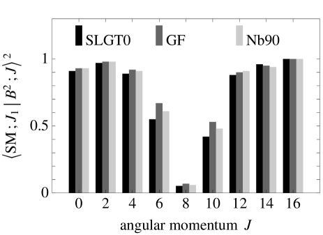
Figure 1: Overlaps of the $(1g_{9/2})^{4}$ yrast eigenstates of the interactions SLGT0, GF, and Nb90 with angular momentum $J$ and isospin $T=0$, with the two-pair state $|B^{2};J\rangle$.

We now analyze the yrast eigenstates of the various interactions defined in Table 1, that is, the quantities $\langle F_{i}|E_{r}\rangle^{2}$ for $r=1$ and a variety of two-pair states $F_{i}$. Pairs with angular momentum $J$ are generically denoted as $P_{J}$ and explicitly, following standard spectroscopic notation, as $S$, $D$, $G$, $I$, and $K$ for $J=0$, 2, 4, 6, and 8. Since this paper deals in particular with the aligned n-p pair with $J=9$, we reserve for it the non-standard notation ‘$B$’ (for Blomqvist). The central result is shown in Fig. 1 which displays the quantity $\langle J_{1}|B^{2};J\rangle^{2}$ where $|J_{1}\rangle$ is the yrast eigenstate with angular momentum $J$ and isospin $T=0$ of the interactions SLGT0, GF, and Nb90. Most yrast states have a large overlap with $B^{2}$, as was shown by Blomqvist, but this is conspicuously not the case for $J\approx 8$. It seems as if the two aligned n-p pairs do not like to couple to a total angular momentum which equals their individual spins.

Table 3: Coefficients $a_{[\Gamma_{1}\Gamma_{2}]\Gamma}^{\lambda}$ in the expansion (45) of the diagonal energies of the $(9/2)^{4}$ system for isospin $T=0$.

		$J=0$			$J=2$			$J=4$			$J=6$			$J=8$			$J=10$
$\lambda$		$[B^{2}]$	$[S^{2}]$		$[B^{2}]$	$[SD]$		$[B^{2}]$	$[SG]$		$[B^{2}]$	$[SI]$		$[B^{2}]$	$[SK]$		$[B^{2}]$	$[DK]$
0		1.14	2.20		0.85	1.20		0.42	1.20		0.11	1.20		0.01	1.20		—	—
1		0.76	0.16		0.64	0.28		0.42	0.24		0.18	0.17		0.04	0.08		0.00	0.02
2		1.70	0.09		1.79	1.30		1.74	0.08		1.26	0.04		0.55	0.07		0.10	1.15
3		0.23	0.38		0.33	0.47		0.50	0.21		0.57	0.28		0.43	0.52		0.18	0.11
4		0.16	0.16		0.34	0.15		0.79	1.26		1.41	0.21		1.76	0.08		1.36	0.10
5		0.01	0.60		0.02	0.39		0.09	0.54		0.24	0.62		0.47	0.68		0.62	0.66
6		0.00	0.24		0.00	0.11		0.05	0.30		0.21	1.29		0.65	0.20		1.42	0.21
7		0.00	0.82		0.00	0.39		0.00	0.94		0.01	0.97		0.06	0.77		0.19	1.18
8		0.00	0.31		0.00	0.23		0.00	0.16		0.00	0.26		0.02	1.45		0.12	1.53
9		2.00	1.04		2.00	1.47		2.00	1.07		2.00	0.96		2.00	0.95		2.00	1.03

To acquire some insight in this finding, we note that simple expressions in terms of the two-body matrix elements are available for the diagonal energies of two-pair states,

$$E(\gamma^{4}[\Gamma_{1}\Gamma_{2}]\Gamma)\equiv\langle\gamma^{4}[\Gamma_{1}\Gamma_{2}]\Gamma|\hat{H}^{\rm F}_{2}|\gamma^{4}[\Gamma_{1}\Gamma_{2}]\Gamma\rangle=\sum_{\lambda}a_{[\Gamma_{1}\Gamma_{2}]\Gamma}^{\lambda}\;\nu_{\lambda},$$ (45)

where the coefficients $a_{[\Gamma_{1}\Gamma_{2}]\Gamma}^{\lambda}$ of relevance to the present discussion are shown in Table 3. According to a recent paper by Talmi Talmi10 , they are non-negative rational numbers; since they involve ratios of rather large integers in this case, Table 3 gives numerical approximations. Of all the coefficients given in this table, the important ones have $\lambda=0$, 1, and 9, because these are the multipolarities of the most attractive interaction matrix elements. It is seen that the contributions of the aligned matrix element ($\lambda=9$) to the energies of the states $|(9/2)^{4}[B^{2}]J\rangle$ and $|(9/2)^{4}[SP_{J}]J\rangle$ remain more or less constant, independent of $J$. This is not the case for the pairing matrix element ($\lambda=0$) whose contribution to the energy of $|(9/2)^{4}[B^{2}]J\rangle$ disappears as $J$ increases while it remains important for $|(9/2)^{4}[SP_{J}]J\rangle$. The combined effect of these contributions is that the state $|(9/2)^{4}[SP_{J}]J\rangle$ dips below $|(9/2)^{4}[B^{2}]J\rangle$ around $J\approx 8$ and as a result picks up the largest component of the yrast eigenstate. Hence, the feature of the disappearing $B$ dominance around $J\approx 8$ is explained by a combination of geometry—the CFPs in the $j=9/2$ orbit, and dynamics—the dependence of the interaction matrix elements on $\lambda$.

Table 4: Overlaps of the $(1g_{9/2})^{4}$ yrast eigenstates of the SLGT0 interaction with angular momentum $J$ and isospin $T=0$ with various two-pair states, expressed in percentages.

$J$	$B^{2}$	$SP_{J}$	$D^{2}$	$DG$	$DI$	$DK$	$G^{2}$	$I^{2}$	$K^{2}$
$0$	91	80	35	—	—	—	18	7.4	1.9
$2$	97	85	17	22	—	—	1.5	0.0	0.4
$4$	89	64	42	11	11	—	0.2	0.2	0.0
$6$	55	70	—	43	0.2	4.3	0.0	0.2	0.0
$8$	5.3	83	—	—	7.4	24	1.8	0.2	0.1
$10$	42	—	—	—	—	58	—	6.1	0.5
$12$	88	—	—	—	—	—	—	57	1.5
$14$	96	—	—	—	—	—	—	—	31.4
$16$	100	—	—	—	—	—	—	—	100

Figure 1 shows that the overlaps $\langle J_{1}|B^{2};J\rangle^{2}$ are very similar for the three interactions. This finding is at the basis of the fact that the subsequent analysis gives consistent results for the three interactions. While there can be significant differences in the shell-model results with the different interactions, the approximation in terms of aligned pairs is similar for the three interactions. In other words, if a particular shell-model state is well approximated in terms of aligned pairs for one interaction, it is so for the other two as well; if the approximation is less good, it is so for all three interactions. Although we have carried out the complete analysis for the three interactions SLGT0, GF, and Nb90, we will show in the following only the results of the former since it has a proven track record of satisfactorily reproducing the data in the mass region of interest Herndl97 .

In Table 4 are shown the amplitudes in percentages for yrast eigenstates of the SLGT0 interaction with even $J$ and $T=0$, that is, the quantities $100\times\langle F_{i}|E_{r}\rangle^{2}$ for $r=1$ and a variety of pair states $|F_{i}\rangle$. The numbers illustrate that, at least at low and at high angular momentum $J$, the overlaps of the physical eigenstates with $|B^{2};J\rangle$ are more important than those with other pair combinations. The percentages shown in Table 4 also illustrate the non-orthogonality of the two-pair basis. For the example, the $J=0$ ground state has a 91% overlap with $B^{2}$ but also a 80% overlap with $S^{2}$; this can only be if the overlap $\langle B^{2}|S^{2}\rangle$ itself is rather large.

IV.3 Boson mappings

Ideally, one would like to perform a similar analysis of shell-model eigenstates for more than four nucleons. That is a challenging problem, however, since it requires the formulation of a nucleon-pair shell model Chen93 ; Chen97 in an isospin-invariant formalism. In this paper we choose to extend our analysis toward higher hole number through the boson mapping techniques explained in Sect. III. It is important to stress that this approximation goes beyond the original proposal of Blomqvist since it involves an additional assumption of the boson character of the fermion pairs. The results presented in this subsection therefore do not directly address Blomqvist’s conjecture.

Once the mapping is carried out for the two- and four-hole systems according to one of the two procedures described in Sect. III, a Hamiltonian is obtained in terms of the selected bosons $\ell_{1},\ell_{2},\dots,\ell_{p}$, which can then be applied to systems with two or more bosons. Such a description shall be referred to as $\ell_{1}\ell_{2}\dots\ell_{p}$-IBM, where IBM stands for interacting boson model Iachello87 . Note that all versions of IBM thus obtained are isospin invariant; for example, the $sd$-IBM is in fact the IBM-3 of Elliott and White Elliott80 .

To compare the merits of different selections of fermion pairs, the following mappings are considered:

1. A single fermion pair $B$ with $J=9,T=0$, leading to the $b$-IBM.

2. Two fermion pairs $S$ and $B$ with $J=0,T=1$ and $J=9,T=0$, leading to the $sb$-IBM.

3. Two fermion pairs $S$ and $D$ with $J=0$ and 2, both with $T=1$, leading to the $sd$-IBM.

4. Three fermion pairs $S$, $D$, and $G$ with $J=0$, 2, and 4, all with $T=1$, leading to the $sdg$-IBM.

The first two cases are inspired by Blomqvist’s conjecture, involving the aligned n-p pair, while the next two are the standard choice of the IBM Iachello87 and its most frequently used extension which includes $g$ bosons. (For a review on the latter, see Ref. Devi92 .)

Table 5: Energies (in MeV) of $T=0$ levels for four nucleons in the $1g_{9/2}$ orbit (⁹⁶Cd) calculated with the shell-model interaction SLGT0 and compared with various versions of IBM obtained by democratic or OAI mapping. $E_{0}$ is the binding energy of the ground state.

		SLGT0		$b$-IBM		$sb$-IBM		$sd$-IBM		$sdg$-IBM
$E_{0}$		9.050		8.643		9.041		8.932		9.050
$0_{1}^{+}$		0		0		0		0		0
$2_{1}^{+}$		0.963		0.678		1.077		1.199		1.002
$4_{1}^{+}$		2.100		1.941		2.339		3.754		2.204
$6_{1}^{+}$		3.079		3.302		3.700		—		4.034
$8_{1}^{+}$		3.449		4.425		4.824		—		5.688
$10_{1}^{+}$		5.227		5.179		5.578		—		—
$12_{1}^{+}$		5.904		5.572		5.971		—		—
$14_{1}^{+}$		6.056		5.692		6.091		—		—
$16_{1}^{+}$		5.904		5.496		5.895		—		—
$18_{1}^{+}$		—		$\infty$		$\infty$		—		—
$0_{2}^{+}$		4.594		—		4.613		4.491		4.594
$2_{2}^{+}$		4.491		—		—		4.730		4.554
$4_{2}^{+}$		4.390		—		—		—		4.538

The results obtained with the various boson Hamiltonians are compared with $T=0$ eigenstates of the SLGT0 interaction for four, six, and eight nucleons in Tables 5, 6, and 7, respectively. The numerical calculations have been performed with the codes ArbModel Heinze and IBM-3 Isacker . The former is a general purpose program that can handle systems of fermions and/or bosons with arbitrary spins and can thus be used for the shell-model as well as the IBM calculations; the latter code is specifically written for the isospin-invariant $sd$-IBM. Alternatively, for three and four identical bosons (i.e., for $b$-IBM) the calculations can be performed with the expressions given in Sect. II and equivalent ones for the three-hole case.

A few remarks are in order. All results concern absolute energies. In the first line of each table are given the binding energies $E_{0}$ of the $T=0$ ground states, as obtained in the various mappings, which should be compared with the corresponding quantity in the shell model. In subsequent lines are given the energies of a selected number of states, relative to this ground state. This might lead to some seemingly counterintuitive results. For example, it is seen from Table 4 that the four-hole $2^{+}_{1}$ shell-model state overlaps 97 % with a $B^{2}$ configuration. Why, then, should its excitation energy come out rather poorly in $b$-IBM (0.678 MeV compared with 0.963 MeV in the shell model, see Table 5)? The reason is that the absolute energy of the $2^{+}_{1}$ state is rather well reproduced (it misses only 0.122 MeV of the shell-model correlation energy) while the absolute energy of the ground state is rather worse underbound (by 0.407 MeV) in $b$-IBM.

Table 6: Energies (in MeV) of $T=0$ levels for six nucleons in the $1g_{9/2}$ orbit (⁹⁴Ag) calculated with the shell-model interaction SLGT0 and compared with various versions of the IBM obtained with two methods of mapping, democratic (Dem) and OAI. $E_{0}$ is the binding energy of the ground state.

		SLGT0		$b$-IBM		$sb$-IBM				$sd$-IBM
						Dem		OAI		Dem		OAI
$E_{0}$		11.276		11.368		11.368		11.368		8.592		8.592
$0_{1}^{+}$		—		—		—		—		—		—
$1_{1}^{+}$		0.126		4.340		4.340		4.340		0		0
$2_{1}^{+}$		1.580		—		—		—		—		—
$3_{1}^{+}$		0.298		3.540		3.540		3.540		0.547		0.547
$4_{1}^{+}$		1.531		3.848		3.848		3.848		—		—
$5_{1}^{+}$		0.674		2.163		2.163		2.163		—		—
$6_{1}^{+}$		1.354		2.352		2.352		2.352		—		—
$7_{1}^{+}$		0		0		0		0		—		—
$8_{1}^{+}$		0.380		0.505		0.505		0.505		—		—
$9_{1}^{+}$		0.432		0.796		0.572		0.538		—		—
$10_{1}^{+}$		1.579		1.784		1.784		1.784		—		—
$11_{1}^{+}$		1.572		1.833		1.833		1.833		—		—
$12_{1}^{+}$		2.933		3.351		3.351		3.351		—		—
$13_{1}^{+}$		2.734		3.220		3.220		3.220		—		—
$14_{1}^{+}$		3.840		4.857		4.857		4.857		—		—
$15_{1}^{+}$		3.577		4.602		4.602		4.602		—		—
$16_{1}^{+}$		5.364		6.029		6.029		6.029		—		—
$17_{1}^{+}$		5.219		5.677		5.677		5.677		—		—
$18_{1}^{+}$		6.606		6.772		6.772		6.772		—		—
$19_{1}^{+}$		6.155		6.324		6.324		6.324		—		—
$20_{1}^{+}$		—		$\infty$		$\infty$		$\infty$		—		—
$21_{1}^{+}$		6.464		6.609		6.609		6.609		—		—

The two-boson spectra obtained from mapping the four-hole shell-model results depend on the kind of pairs included in the basis but otherwise they are identical in the OAI and democratic mappings. Therefore, for each of the different IBM versions, there is a unique spectrum shown in Table 5 which is identical to that of the shell-model hamiltonian when diagonalized in the corresponding (possibly truncated) two-pair basis. While the OAI and democratic mappings yield the same energy spectrum for four holes, they lead to different boson-boson interaction matrix elements. Hence, the OAI and democratic results are different for the six- and eight-hole spectra shown in Tables 6 and 7.

If the number of two-pair states equals the number of independent four-hole shell-model states, then the two-boson calculation reproduces the four-hole results exactly. According to Table 5 this happens, for example, for the three $J^{\pi}=0^{+}$ states with $T=0$ which can be exactly described as combinations of $|S^{2};0\rangle$, $|D^{2};0\rangle$, and $|G^{2};0\rangle$. Consequently, the three shell-model $0^{+}$ states are exactly reproduced in $sdg$-IBM.

Because of the Pauli exclusion principle, no four-hole shell-model state exists with $J=18$ while this angular momentum is allowed in the coupling of two bosons with $J=9$. This is an example of the complication mentioned at the end of Sect. III and the solution given there should be applied. In this case it implies that the matrix element $\langle B^{2};18|\hat{H}^{\rm B}_{2}|B^{2};18\rangle$ should be taken infinitely repulsive and it is only by adhering to this procedure that reasonable results can be obtained.

Not much is known experimentally about ⁹⁴Ag except for the presence of two isomers, with tentative spin-parity assignments $7^{+}$ (presumably the lowest $T=0$ state) and $21^{+}$ at about $5.78(3)$ MeV above the $7^{+}$ Mukha05 . The different shell-model interactions SLGT0, GF, and Nb90 all predict a $7^{+}$ as the $T=0$ ground state, and a $21^{+}$ level at 6.464, 5.948, and 4.632 MeV, respectively. The $b$-IBM reproduces the shell-model result for the binding energies of these isomers to about 100 keV for the $7^{+}$ and less than that for the $21^{+}$ (see Table 6 for the results of the SLGT0 interaction). This result is valid for the different shell-model interactions: although the binding energies calculated with the three shell-model interactions vary by several MeV, in each case they are matched by the (appropriately mapped) $b$-IBM to within about 100 keV, indicating that the $B$ pair incorporates most of the correlations for the $7^{+}$ and $21^{+}$ states.

The $b$-IBM results should be contrasted to those obtained with $sd$-IBM which fails completely to reproduce the spectroscopy of ⁹⁴Ag. This is not surprising since it is known from the work of Elliott and Evans Elliott81 that IBM-3 cannot give a satisfactory description of odd-odd nuclei which require the addition of isoscalar $s$ and $d$ bosons leading to the so-called IBM-4. While the latter is a realistic model when low-$j$ shell-model orbits are involved (e.g., for $sd$-shell nuclei Halse84 ; Halse85 ), the present results seem to indicate that the mapping from a shell-model space with high-$j$ orbits calls for the inclusion of an aligned isoscalar n-p pair with $J=2j$.

Table 7: Energies (in MeV) of $T=0$ levels for eight nucleons in the $1g_{9/2}$ orbit (⁹²Pd) calculated with the shell-model interaction SLGT0 and compared with various versions of the IBM obtained with two methods of mapping, democratic (Dem) and OAI. $E_{0}$ is the binding energy of the ground state.

		SLGT0		$b$-IBM		$sb$-IBM				$sd$-IBM
						Dem		OAI		Dem		OAI
$E_{0}$		18.937		18.135		18.771		18.646		18.624		19.999
$0_{1}^{+}$		0		0		0		0		0		0
$2_{1}^{+}$		0.927		0.637		1.170		0.917		0.728		0.762
$4_{1}^{+}$		1.728		1.104		1.740		1.608		1.561		2.054
$6_{1}^{+}$		2.512		1.965		2.628		2.441		3.155		4.267
$8_{1}^{+}$		3.198		2.836		3.501		3.320		5.486		6.861
$10_{1}^{+}$		4.233		3.683		4.325		4.185		—		—
$12_{1}^{+}$		5.123		4.414		5.050		4.924		—		—

While $b$-IBM and $sb$-IBM are largely equivalent for the odd-odd nucleus ⁹⁴Ag, this is not the case for the even-even nucleus ⁹²Pd. As can be seen from Table 7, the $s$ boson provides crucial additional correlation energy which brings the boson result close to its shell-model equivalent. This nucleus was studied recently in a fusion-evaporation experiment Cederwall10 . The excitation energies of the yrast levels, calculated with the SLGT0 interaction, are in reasonable agreement with the observed values of 0.874, 1.786, and 2.535 MeV, respectively.

IV.4 Electric quadrupole properties

A further test of the aligned-n-p-pair hypothesis can be obtained from electric quadrupole (E2) transition properties. The E2 operator in the shell model is given by

$$\hat{T}^{\rm F}_{\mu}({\rm E}2)=e_{\nu}\sum_{i\in\nu}r_{i}^{2}Y_{2\mu}(\theta_{i},\phi_{i})+e_{\pi}\sum_{i\in\pi}r_{i}^{2}Y_{2\mu}(\theta_{i},\phi_{i}),$$ (46)

where the sums are over neutrons and protons, and each sum is multiplied with the appropriate effective charge. This operator can be written alternatively as a sum of an isoscalar operator, multiplied by $(e_{\nu}+e_{\pi})$, and an isovector operator, multiplied by $(e_{\nu}-e_{\pi})$. For the E2 transitions between $T=0$ levels of interest here, only the former part contributes. In second quantization, which is a convenient formalism for carrying out the mapping, the fermion E2 operator can be written as

$$\hat{T}^{\rm F}_{\mu}({\rm E}2)=-\sqrt{\frac{55}{3\pi}}l_{\rm ho}^{2}\left[e_{\nu}(a^{\dagger}_{\nu}\times\tilde{a}_{\nu})^{(2)}_{\mu}+e_{\pi}(a^{\dagger}_{\pi}\times\tilde{a}_{\pi})^{(2)}_{\mu}\right],$$ (47)

where $a^{\dagger}_{\rho}$ creates a neutron ($\rho=\nu$) or a proton ($\rho=\pi$) in the $1g_{9/2}$ orbit, and $\tilde{a}_{jm}=(-)^{j+m}a_{j-m}$. Furthermore, the factor in front comes from the radial integral over harmonic-oscillator wave functions (with length parameter $l_{\rm ho}$) involving the $1g_{9/2}$ orbit.

The lowest-order bosonic image of the fermion E2 operator is defined by the diagonal (reduced) matrix element in the $9^{+}$ state of the 1n-1p system which is given by

$$\langle(1g_{9/2})^{2};9^{+}||\hat{T}^{\rm F}({\rm E}2)||(1g_{9/2})^{2};9^{+}\rangle=-\sqrt{\frac{55}{3\pi}}l_{\rm ho}^{2}\times\sqrt{\frac{1330}{187}}(e_{\nu}+e_{\pi}).$$ (48)

The E2 operator of the $b$-IBM is of the form

$$\hat{T}^{\rm B}_{\mu}({\rm E}2)=e_{\rm b}(b^{\dagger}\times\tilde{b})^{(2)}_{\mu},$$ (49)

and is necessarily of scalar character in isospin. Since the mapping implies the equality

$$\langle(1g_{9/2})^{2};9^{+}||\hat{T}^{\rm F}({\rm E}2)||(1g_{9/2})^{2};9^{+}\rangle=\langle b||\hat{T}^{\rm B}({\rm E}2)||b\rangle,$$ (50)

and the since the boson matrix element on the right-hand side equals $\sqrt{5}e_{\rm b}$, we find the following expression of the boson effective charge $e_{\rm b}$ in terms of the shell-model neutron and proton effective charges:

$$e_{\rm b}=-\sqrt{\frac{55}{3\pi}}l_{\rm ho}^{2}\times\sqrt{\frac{266}{187}}(e_{\nu}+e_{\pi}).$$ (51)

In the following, the factor $\sqrt{55/3\pi}(e_{\nu}+e_{\pi})l_{\rm ho}^{2}$ is divided out of all matrix elements, fermionic as well bosonic.

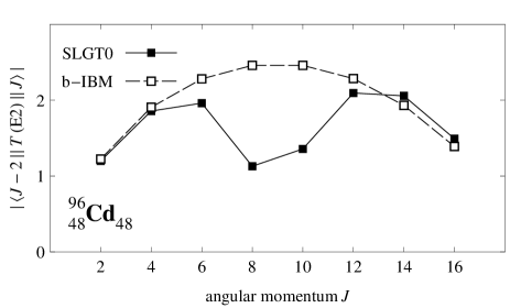
Figure 2: Absolute values of the E2 reduced matrix elements for the transitions $J\rightarrow J-2$ between four-nucleon-hole states with $T=0$ in the $1g_{9/2}$ orbit (⁹⁶Cd), calculated with the SLGT0 shell-model interaction and compared with the mapped $b$-IBM. Matrix elements are expressed in units $\sqrt{55/3\pi}(e_{\nu}+e_{\pi})l_{\rm ho}^{2}$ (see text).

A first test is from E2 transitions between four-nucleon-hole states with $T=0$. The shell-model results obtained with the SLGT0 interaction, shown in Fig. 2, display a characteristic decrease in quadrupole strength for $J\approx 8$ which can be viewed as a remnant of a seniority-like classification. The figure also shows the results found in $b$-IBM using the boson effective charge derived in Eq. (51), with no adjustable parameter. Not surprisingly, given that the $J=8$ state is poorly described in terms of aligned n-p pairs (and hence $b$ bosons), the two transitions involving this state deviate strongly in $b$-IBM from the corresponding shell-model result. Other transitions agree, however.

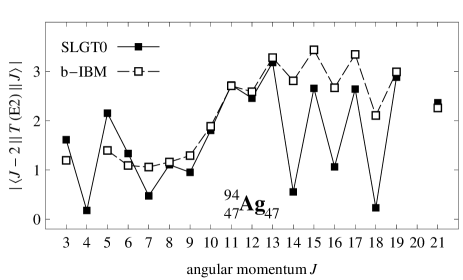
Figure 3: Absolute values of the E2 reduced matrix elements for the transitions $J\rightarrow J-2$ between six-nucleon-hole states with $T=0$ in the $1g_{9/2}$ orbit (⁹⁴Ag), calculated with the SLGT0 shell-model interaction and compared with the mapped $b$-IBM. Matrix elements are expressed in units $\sqrt{55/3\pi}(e_{\nu}+e_{\pi})l_{\rm ho}^{2}$ (see text).

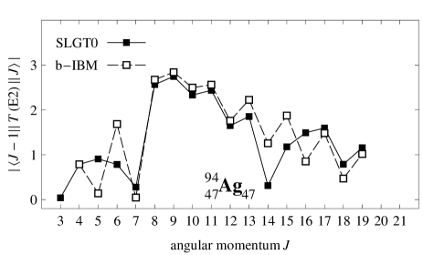
Figure 4: Same caption as Fig. 3 for $J\rightarrow J-1$ transitions.

A second test is provided by E2 transitions between six-nucleon-hole states with $T=0$. They are shown in Figs. 3 and 4 for $J\rightarrow J-2$ and $J\rightarrow J-1$, respectively. Assuming that an agreement between shell model and $b$-IBM is obtained only if both the initial and final states are adequately represented by $b$ bosons, we conclude that the $b$-IBM is a good approximation for two ranges of angular momenta, namely $J=6$ to 13 and $J=17$ to 21. This conclusion agrees, at least qualitatively, with the one drawn on the basis of energies (see Table 7). Since three $b$ bosons cannot couple to total angular momentum $J=2$, this state is absent from $b$-IBM while it is present in the shell model (see Table 7). As a consequence, no $4\rightarrow 2$ or $3\rightarrow 2$ transitions occur in $b$-IBM (see Figs. 3 and 4). These transitions exist in the shell model but it is rather striking that the calculated matrix elements are very small indeed.

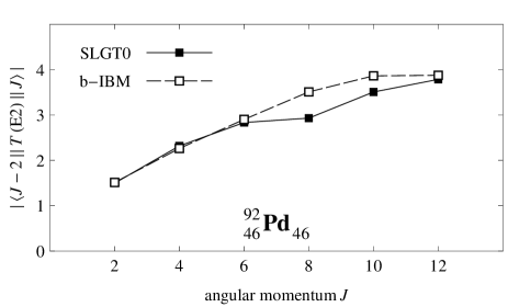
Figure 5: Same caption as Fig. 2 for eight-nucleon-hole states (⁹²Pd).

Finally, in Fig. 5 are shown the E2 transitions between eight-nucleon-hole states with $T=0$. A small depletion of the E2 strength calculated in the shell model is perceptible for $J\approx 8$ and is absent in $b$-IBM. Apart from this deviation both calculations agree, indicating that the shell-model wave functions can be adequately represented in terms of a single $b$ boson. We emphasize once more that, the number of states that can be written in terms of $B$ pairs is small (of the order of 10), no effective charges are needed to arrive at the agreement in Fig. 5.

Let us now formulate an overall evaluation of these results. While the $b$-IBM gives in all cases an reasonable description of the ground-state binding energy, the addition of the standard $s$ boson (with $J=0,T=1$) further improves the agreement. In fact, the energies obtained in $sb$-IBM (both with the OAI and democratic mappings) agree well with those of the shell-model levels except for (i) the $J=8$ level in the four-hole system, (ii) low-$J$ levels of the six-hole system, and (iii) levels with $J=14$ to 16 in the six-hole system. The first discrepancy is obviously related to the small overlap of the $J=8$ shell-model state with $|B^{2};J=8\rangle$, noted in Table 4 and explained in Sect. IV.2. The second difference is also understandable since a correct description of the low-$J$ states in the odd-odd nucleus ⁹⁴Ag requires the consideration of low-$J$ pairs with $T=0$ which have been omitted from the present mapping. The third deviation could be related to an unfavorable coupling of three $B$ pairs to the angular momenta $J=14$, 15, and 16, akin to the coupling of two $B$ pairs to $J=8$. The results as regards E2 transitions are consistent with what is concluded from the analysis of spectra.

V Conclusions

We have shown in this paper that part of the low-energy spectroscopy of $N=Z$ nuclei which have their valence nucleons confined to a single high-$j$ orbit, can be represented in terms of an aligned isoscalar n-p $B$ pair with $J=2j$ and is further improved by the inclusion of an isovector $S$ pair coupled to $J=0$. This was proven explicitly for a four-hole system and indirectly, through a mapping onto a corresponding boson system, for six and eight holes. Some deficiencies were found in this approach. A first concerns states of the four-hole system with angular momentum $J\approx 2j$ which turn out to be poorly approximated with just $S$ and $B$ pairs. A second deficiency is more generic and pertains to the low-$J$ states in odd-odd $N=Z$ nuclei, the description of which calls for the inclusion of isoscalar n-p pairs with low angular momentum. Nevertheless, it should be noted that the two isomers that have been observed so far in ⁹⁴Ag, $(7^{+})$ and $(21^{+})$, are adequately described in terms of $b$ bosons.

These results were obtained for the $1g_{9/2}$ orbit and for three different choices of two-body interaction. To what extent are they valid in general and can they be considered as representative of a system of neutrons and protons confined to a high-$j$ orbit? In essence, two ingredients, geometry and dynamics, determine the outcome of the present pair analysis. The geometry is defined by the CFPs and, provided $j$ is not too small, is expected to evolve only slowly with $j$. (It would in fact be an exercise of some interest to perform the pair analysis in the limit of large $j$.) The dynamics is determined by the two-body interaction which in our study was varied significantly but within reasonable bounds. The matrix elements shown in Table 1 are typical of what is obtained for a residual interaction with a short-range, attractive character Schiffer76 and we may thus expect similar results when we move to orbits other than $1g_{9/2}$.

This work calls for further studies. The pair analysis of the shell-model wave functions should be extended to higher particle numbers which can be achieved through an isospin-invariant formulation of the nucleon-pair shell model. Consequently, the present results require further confirmation at higher particle number but one is tempted to conclude at this point that a realistic model can be formulated in terms of $s$ and $b$ bosons. Due to its simplicity, such a model could be of use to elucidate the main structural features of $N\sim Z$ nuclei in this mass region. These topics are currently under study.

We wish to thank Stefan Heinze for his help with the numerical calculations with ArbModel and Aurore Dijon for her help with the shell-model calculations. This work has been carried out in the framework of CNRS/DEF project N 19848. S.Z. thanks the Algerian Ministry of High Education and Scientific Research for financial support. This work was also partially supported by the Agence Nationale de Recherche, France, under contract nr ANR-07-BLAN-0256-03.

References

- (1) D.D. Warner, M. Bentley, and P. Van Isacker, Nature Phys. 2, 311 (2006).
- (2) O. Juillet and S. Josse, Eur. Phys. J. A 8, 291 (2000).
- (3) B. Cederwall et al., Nature 469, 68 (2011).
- (4) J. Blomqvist, private communication.
- (5) M. Danos and V. Gillet, Phys. Rev. 161, 1034 (1967).
- (6) I. Talmi, Simple Models of Complex Nuclei. The Shell Model and Interacting Boson Model (Harwood, Academic, Chur, Switzerland, 1993).
- (7) T. Otsuka, A. Arima, and F. Iachello, Nucl. Phys. A 309, 1 (1978).
- (8) L. D. Skouras, P. Van Isacker, and M. A. Nagarajan, Nucl. Phys. A 516, 255 (1990).
- (9) E. J. D. Serduke, R. D. Lawson, and D. H. Gloeckner, Nucl. Phys. A 256, 45 (1976).
- (10) H. Herndl and B. A. Brown, Nucl. Phys. A 627, 35 (1997).
- (11) R. Gross and A. Frenkel, Nucl. Phys. A 267, 85 (1976).
- (12) National Nuclear Data Center (NNDC), http://www.nndc.bnl.gov/
- (13) G. Audi, A. H. Wapstra, and C. Thibault, Nucl. Phys. A 729, 337 (2003).
- (14) D. Lunney, J. M. Pearson, and C. Thibault, Rev. Mod. Phys. 75, 1021 (2003).
- (15) M.-G. Porquet, private communication.
- (16) C. A. Fields, R. A. Ristinen, L. E. Samuelson, and P. A. Smith, Nucl. Phys. A 385, 449 (1982).
- (17) S. P. Pandya, Phys. Rev. 103, 956 (1956).
- (18) O. Sorlin and M.-G. Porquet, Progr. Part. Nucl. Phys. 61, 602 (2008).
- (19) C. J. Lister et al., Phys. Rev. Lett. 59, 1270 (1987).
- (20) I. Talmi, Nucl. Phys. A 846, 31 (2010).
- (21) J.-Q. Chen, Nucl. Phys. A 562, 218 (1993).
- (22) J.-Q. Chen, Nucl. Phys. A 626, 686 (1997).
- (23) F. Iachello and A. Arima, The Interacting Boson Model (Cambridge University Press, Cambridge, 1987).
- (24) Y. D. Devi and V. K. B. Kota, Pramana J. Phys. 39 1992 (413).
- (25) J. P. Elliott and A. P. White, Phys. Lett. B 97, 169 (1980).
- (26) S. Heinze, program ArbModel, University of Köln, unpublished.
- (27) P. Van Isacker, program IBM-3, unpublished.
- (28) I. Mukha et al., Phys. Rev. Lett. 95, 022501 (2005).
- (29) J. P. Elliott and J. A. Evans, Phys. Lett. B 101, 216 (1981).
- (30) P. Halse, J. P. Elliott and J. A. Evans, Nucl. Phys. A 417, 301 (1984).
- (31) P. Halse, Nucl. Phys. A 445, 93 (1985).
- (32) J.P. Schiffer and W.W. True, Rev. Mod. Phys. 48, 191 (1976).