Abstract

In our work on the development of a model–independent data analysis method for estimating the spin–independent (SI) scalar coupling of Weakly Interacting Massive Particles (WIMPs) on nucleons by using measured recoil energies from direct Dark Matter detection experiments directly, it was assumed that the analyzed data sets are background–free, i.e., all events are WIMP signals. In this article, as a more realistic study, we take into account a fraction of possible residue background events, which pass all discrimination criteria and then mix with other real WIMP–induced events in our data sets. Our simulations show that, for the estimation of the SI WIMP–nucleon coupling, the maximal acceptable fraction of residue background events in the analyzed data set of ${\cal O}(50)$ total events is $\sim$ 10% – 20%. For a WIMP mass of 100 GeV and 20% residue background events, the systematic deviation of the reconstructed SI WIMP coupling (with a reconstructed WIMP mass) would in principle be $\sim+13\%$ with a statistical uncertainty of $\sim^{+21\%}_{-14\%}$ ($\sim-3.3\%^{+18\%}_{-13\%}$ for background–free data sets).

1 Introduction

Currently, direct Dark Matter detection experiments searching for Weakly Interacting Massive Particles (WIMPs) are one of the promising methods for understanding the nature of Dark Matter (DM) and identifying them among new particles produced at colliders as well as reconstructing the (sub)structure of our Galactic halo [1, 2, 3, 4]. To this aim, model–independent methods for determining the WIMP mass [5, 6] as well as estimating the spin–independent (SI) WIMP coupling on nucleons [7, 8] from direct detection experiments have been developed.

These methods built basically on the work on the reconstruction of the (moments of the) one–dimensional velocity distribution function of halo WIMPs by using experimental data (measured recoil energies) directly [12]. The spectrum of recoil energy is proportional to an integral over the one–dimensional WIMP velocity distribution, $f_{1}(v)$, where $v$ is the absolute value of the WIMP velocity in the laboratory frame. In fact, this integral is just the minus–first moment of the velocity distribution function, which can be estimated from experimental data directly [12, 6]. Then, by assuming that the SI WIMP–nucleus interaction dominates and the WIMP couplings on protons and on neutrons are approximately equal, this SI WIMP coupling on nucleons can be estimated from experimental data directly [7, 8]. It was found that, by combining experimental data sets with different target nuclei, the SI WIMP–nucleon coupling can be estimated without making any assumption about the velocity distribution of halo WIMPs nor prior knowledge about the WIMP mass [7, 8].

In the work on the development of these model–independent data analysis procedures for extracting WIMP properties from direct detection experiments, it was assumed that the analyzed data sets are background–free, i.e., all events are WIMP signals. Active background discrimination techniques should make this condition possible. For example, the ratio of the ionization to recoil energy, the so–called “ionization yield”, used in the CDMS-II experiment provides an event–by–event rejection of electron recoil events to be better than $10^{-4}$ misidentification [18]. By combining the “phonon pulse timing parameter”, the rejection ability of the misidentified electron recoils (most of them are “surface events” with sufficiently reduced ionization energies) can be improved to be $<10^{-6}$ [18]. Moreover, as demonstrated by the CRESST collaboration [19], by means of inserting a scintillating foil, which causes some additional scintillation light for events induced by $\alpha$-decay of ${}^{210}{\rm Po}$ and thus shifts the pulse shapes of these events faster than pulses induced by WIMP interactions in the crystal, the pulse shape discrimination (PSD) technique can then easily distinguish WIMP–induced nuclear recoils from those induced by backgrounds.

However, as the most important issue in all underground experiments, the signal identification ability and possible residue background events which pass all discrimination criteria and then mix with other real WIMP–induced events in analyzed data sets should also be considered. Therefore, in this article, as a more realistic study, we follow our works on the effects of residue background events in direct Dark Matter detection experiments [23, 24] and want to study how well we could estimate the SI WIMP–nucleon coupling model–independently by using “impure” data sets and how “dirty” these data sets could be to be still useful.

The remainder of this article is organized as follows. In Sec. 2 I review the model–independent method for estimating the SI WIMP coupling on nucleons by using experimental data sets directly. In Sec. 3 the effects of residue background events in the analyzed data sets on the measured energy spectrum as well as on the reconstructed WIMP mass will briefly be discussed. In Sec. 4 I show numerical results of the reconstructed SI WIMP–nucleon coupling by using mixed data sets with different fractions of residue background events based on Monte Carlo simulations. I conclude in Sec. 5. Some technical details will be given in an appendix.

2 Method for estimating the SI WIMP–nucleon coupling

The basic expression for the differential event rate for elastic WIMP–nucleus scattering is given by [3]:

$$\frac{dR}{dQ}={\cal A}F^{2}(Q)\int_{v_{\rm min}}^{v_{\rm max}}\left[\frac{f_{1}(v)}{v}\right]dv~{}\!.$$ (1)

Here $R$ is the direct detection event rate, i.e., the number of events per unit time and unit mass of detector material, $Q$ is the energy deposited in the detector, $F(Q)$ is the elastic nuclear form factor, $f_{1}(v)$ is the one–dimensional velocity distribution function of the WIMPs impinging on the detector, $v$ is the absolute value of the WIMP velocity in the laboratory frame. The constant coefficient ${\cal A}$ is defined as

$${\cal A}\equiv\frac{\rho_{0}\sigma_{0}}{2m_{\chi}m_{\rm r,N}^{2}}~{}\!,$$ (2)

where $\rho_{0}$ is the WIMP density near the Earth and $\sigma_{0}$ is the total cross section ignoring the form factor suppression. The reduced mass $m_{\rm r,N}$ is defined by

$$m_{\rm r,N}\equiv\frac{m_{\chi}m_{\rm N}}{m_{\chi}+m_{\rm N}}~{}\!,$$ (3)

where $m_{\chi}$ is the WIMP mass and $m_{\rm N}$ that of the target nucleus. Finally, $v_{\rm min}$ is the minimal incoming velocity of incident WIMPs that can deposit the energy $Q$ in the detector:

$$v_{\rm min}=\alpha\sqrt{Q}~{}\!,$$ (4)

with the transformation constant

$$\alpha\equiv\sqrt{\frac{m_{\rm N}}{2m_{\rm r,N}^{2}}}~{}\!,$$ (5)

and $v_{\rm max}$ is the maximal WIMP velocity in the Earth’s reference frame, which is related to the escape velocity from our Galaxy at the position of the Solar system, $v_{\rm esc}~{}\>\raisebox{-3.01385pt}{$\stackrel{{\scriptstyle\textstyle>}}{{\sim}}$}\>~{}600$ km/s.

For spin–independent scalar WIMP interactions, the total cross section in Eq. (2) can be expressed as [3, 4]

$$\sigma_{0}^{\rm SI}=\left(\frac{4}{\pi}\right)m_{\rm r,N}^{2}\Big{[}Zf_{\rm p}+(A-Z)f_{\rm n}\Big{]}^{2}~{}\!.$$ (6)

Here $m_{\rm r,N}$ is the reduced mass defined in Eq. (3), $Z$ is the atomic number of the target nucleus, i.e., the number of protons, $A$ is the atomic mass number, $A-Z$ is then the number of neutrons, $f_{\rm(p,n)}$ are the effective scalar couplings of WIMPs on protons p and on neutrons n, respectively. Here we have to sum over the couplings on each nucleon before squaring because the wavelength associated with the momentum transfer is comparable to or larger than the size of the nucleus, the so–called “coherence effect”. In addition, for the lightest supersymmetric neutralino, and for all WIMPs which interact primarily through Higgs exchange, the scalar couplings are approximately the same on protons and on neutrons: $f_{\rm n}\simeq f_{\rm p}$. Thus the “pointlike” cross section $\sigma_{0}^{\rm SI}$ in Eq. (6) can be written as

$$\sigma_{0}^{\rm SI}\simeq\left(\frac{4}{\pi}\right)m_{\rm r,N}^{2}A^{2}|f_{\rm p}|^{2}=A^{2}\left(\frac{m_{\rm r,N}}{m_{\rm r,p}}\right)^{2}\sigma_{\chi{\rm p}}^{\rm SI}~{}\!,$$ (7)

where $m_{\rm r,p}$ is the reduced mass of the WIMP mass $m_{\chi}$ and the proton mass $m_{\rm p}$, and

$$\sigma_{\chi{\rm p}}^{\rm SI}=\left(\frac{4}{\pi}\right)m_{\rm r,p}^{2}|f_{\rm p}|^{2}$$ (8)

is the SI WIMP–nucleon cross section. Here the tiny mass difference between a proton and a neutron has been neglected.

It was found that, by using a time–averaged recoil spectrum, and assuming that no directional information exists, the normalized one–dimensional velocity distribution function of halo WIMPs, $f_{1}(v)$, can be solved from Eq. (1) analytically [12] and, consequently, its generalized moments can be estimated by [12, 6]

$$\langle{\textstyle{v^{n}}}\rangle(v(Q_{\rm min}),v(Q_{\rm max})) = \int_{v(Q_{\rm min})}^{v(Q_{\rm max})}v^{n}f_{1}(v)~{}\!dv$$ (9)

$$= \alpha^{n}\left[\frac{2Q_{\rm min}^{(n+1)/2}r(Q_{\rm min})/F^{2}(Q_{\rm min})+(n+1)I_{n}(Q_{\rm min},Q_{\rm max})}{2Q_{\rm min}^{1/2}r(Q_{\rm min})/F^{2}(Q_{\rm min})+I_{0}(Q_{\rm min},Q_{\rm max})}\right]~{}\!.$$

Here $v(Q)=\alpha\sqrt{Q}$, $Q_{\rm(min,max)}$ are the experimental minimal and maximal cut–off energies of the data set, respectively,

$$r(Q_{\rm min})\equiv\left(\frac{dR}{dQ}\right)_{{\rm expt},~{}\!Q=Q_{\rm min}}$$ (10)

is an estimated value of the measured recoil spectrum $(dR/dQ)_{\rm expt}$ (before normalized by an experimental exposure $\cal E$) at $Q=Q_{\rm min}$, and $I_{n}(Q_{\rm min},Q_{\rm max})$ can be estimated through the sum:

$$I_{n}(Q_{\rm min},Q_{\rm max})=\sum_{a=1}^{N_{\rm tot}}\frac{Q_{a}^{(n-1)/2}}{F^{2}(Q_{a})}~{}\!,$$ (11)

where the sum runs over all events in the data set that satisfy $Q_{a}\in[Q_{\rm min},Q_{\rm max}]$ and $N_{\rm tot}$ is the number of such events. Note that, firstly, by using the second line of Eq. (9) $\langle{\textstyle{v^{n}}}\rangle(v(Q_{\rm min}),v(Q_{\rm max}))$ can be determined independently of the local WIMP density $\rho_{0}$, of the velocity distribution function of incident WIMPs, $f_{1}(v)$, as well as of the WIMP–nucleus cross section $\sigma_{0}$. Secondly, $r(Q_{\rm min})$ and $I_{n}(Q_{\rm min},Q_{\rm max})$ are two key quantities for our analysis, which can be estimated either from a functional form of the recoil spectrum or from experimental data (i.e., the measured recoil energies) directly.

By substituting the first expression in Eq. (7) into Eq. (1), and using the fact that the integral over the one–dimensional WIMP velocity distribution on the right–hand side of Eq. (1) is the minus–first moment of this distribution, which can be estimated by Eq. (9) with $n=-1$, we have

$$\left(\frac{dR}{dQ}\right)_{{\rm expt},~{}\!Q=Q_{\rm min}} = {\cal E}{\cal A}F^{2}(Q_{\rm min})\int_{v(Q_{\rm min})}^{v(Q_{\rm max})}\left[\frac{f_{1}(v)}{v}\right]dv$$ (12)

$$= {\cal E}\left(\frac{2\rho_{0}A^{2}|f_{\rm p}|^{2}}{\pi m_{\chi}}\right)F^{2}(Q_{\rm min})\cdot\frac{1}{\alpha}\left[\frac{2r(Q_{\rm min})/F^{2}(Q_{\rm min})}{2Q_{\rm min}^{1/2}r(Q_{\rm min})/F^{2}(Q_{\rm min})+I_{0}}\right]~{}\!.$$

Using the definition (5) of $\alpha$, the squared SI WIMP coupling on protons (nucleons) can then be expressed as [7, 8]

$$|f_{\rm p}|^{2}=\frac{1}{\rho_{0}}\left[\frac{\pi}{4\sqrt{2}}\left(\frac{1}{{\cal E}A^{2}\sqrt{m_{\rm N}}}\right)\right]\left[\frac{2Q_{\rm min}^{1/2}r(Q_{\rm min})}{F^{2}(Q_{\rm min})}+I_{0}\right]\left(m_{\chi}+m_{\rm N}\right)~{}\!.$$ (13)

Note that the experimental exposure ${\cal E}$ appearing in the denominator relates the actual counting rate $(dR/dQ)_{\rm expt}$ to the normalized rate in Eq. (1).

As mentioned in the introduction, the Dark Matter density at the position of the Solar system, $\rho_{0}$, appearing in the denominator of the expression (13) for estimating $|f_{\rm p}|^{2}$ has conventionally been estimated by means of the measurement of the rotation curve of the Milky Way. The currently most commonly used value for $\rho_{0}$ is [3, 4]

$$\rho_{0}\approx 0.3~{}{\rm GeV/cm^{3}}~{}\!,$$ (14)

with an uncertainty of a factor of $\sim$ 2. However, some new techniques have been developed for determining $\rho_{0}$ with a higher precision [13, 14, 15, 16, 17]. These estimates give rather larger values for $\rho_{0}$; e.g., Catena and Ullio gave [13]

$$\rho_{0}=0.39\pm 0.03~{}{\rm GeV/cm^{3}}~{}\!,$$ (15)

and Salucci et al. even gave [15]

$$\rho_{0}=0.43\pm 0.11\pm 0.10~{}{\rm GeV/cm^{3}}~{}\!.$$ (16)

Moreover, instead of a spherical symmetric density profile assumed in Refs. [13, 15], in Refs. [14, 16, 17] the authors considered an axisymmetric density profile for a flattened Galactic Dark Matter halo [25] caused by the disk structure of the luminous baryonic component. It was found that the local density of such a non–spherical DM halo could be enhanced by $\sim$ 20% or larger [14, 16] and Pato et al. gave therefore [16]

$$\rho_{0}=0.466\pm 0.033({\rm stat})\pm 0.077({\rm syst})~{}{\rm GeV/cm^{3}}~{}\!.$$ (17)

Nevertheless, since the squared SI WIMP–nucleon coupling $|f_{\rm p}|^{2}$ is inversely proportional to the local WIMP density, by using Eq. (13) one can at least give an upper bound on $|f_{\rm p}|^{2}$. Moreover, as shown in Refs. [7, 8], in spite of the very few ($\cal O$(50)) events from one experiment, for a WIMP mass of 100 GeV, the SI WIMP–nucleon coupling $|f_{\rm p}|$ can be estimated with a statistical uncertainty of only $\sim$ 15%; it leads to an uncertainty on the SI WIMP–nucleon cross section of $\sim$ 30%, which is (much) smaller than the uncertainty on the estimate of the local Dark Matter density.

3 Effects of residue background events

In this section I first show some numerical results of the energy spectrum of WIMP recoil signals mixed with a few background events. Then I review the effects of residue background events in the analyzed data sets on the reconstruction of the WIMP mass $m_{\chi}$.

For generating WIMP–induced signals, we use the shifted Maxwellian velocity distribution [2, 3, 12]:

$$f_{1,{\rm sh}}(v)=\frac{1}{\sqrt{\pi}}\left(\frac{v}{v_{\rm e}v_{0}}\right)\bigg{[}e^{-(v-v_{\rm e})^{2}/v_{0}^{2}}-e^{-(v+v_{\rm e})^{2}/v_{0}^{2}}\bigg{]}~{}\!,$$ (18)

with $v_{0}\simeq 220~{}{\rm km/s}$ and $v_{\rm e}=1.05~{}\!v_{0}$, which are the Sun’s orbital velocity and the Earth’s velocity in the Galactic frame, respectively; the maximal cut–off of the velocity distribution function has been set as $v_{\rm max}=700$ km/s. The commonly used elastic nuclear form factor for the SI cross section [26, 3, 4]:

$$F_{\rm SI}^{2}(Q)=\left[\frac{3j_{1}(qR_{1})}{qR_{1}}\right]^{2}e^{-(qs)^{2}}$$ (19)

will also be used. Meanwhile, in order to check the need of a prior knowledge about an (exact) form of the residue background spectrum, two forms for the background spectrum have been considered. The simplest choice is a constant spectrum:

$$\left(\frac{dR}{dQ}\right)_{\rm bg,const}=1~{}\!.$$ (20)

More realistically, we use the target–dependent exponential form introduced in Ref. [23] for the residue background spectrum:

$$\left(\frac{dR}{dQ}\right)_{\rm bg,ex}=\exp\left(-\frac{Q/{\rm keV}}{A^{0.6}}\right)~{}\!.$$ (21)

Here $Q$ is the recoil energy, $A$ is the atomic mass number of the target nucleus. The power index of $A$, 0.6, is an empirical constant, which has been chosen so that the exponential background spectrum is somehow similar to, but still different from the expected recoil spectrum of the target nucleus; otherwise, there is in practice no difference between the WIMP scattering and background spectra. Note that, among different possible choices, we use in our simulations the atomic mass number $A$ as the simplest, unique characteristic parameter in the general analytic form (21) for defining the residue background spectrum for different target nuclei. However, it does not mean that the (superposition of the real) background spectra would depend simply/primarily on $A$ or on the mass of the target nucleus, $m_{\rm N}$. In other words, it is practically equivalent to use expression (21) or $(dR/dQ)_{\rm bg,ex}=e^{-Q/13.5~{}{\rm keV}}$ directly for a ${}^{76}{\rm Ge}$ target.

Note also that, firstly, as argued in Ref. [23], two forms of background spectrum given above are rather naive; however, since we consider here only a few residue background events induced by perhaps two or more different sources, which pass all discrimination criteria, and then mix with other WIMP–induced events in our data sets of ${\cal O}(50)$ total events, exact forms of different background spectra are actually not very important and these two spectra, in particular, the exponential one, should practically not be unrealistic. Secondly, as demonstrated in Refs. [7, 8] and reviewed in the previous section, the model–independent data analysis procedure for estimating the SI WIMP–nucleon coupling requires only measured recoil energies (induced mostly by WIMPs and occasionally by background sources) from direct detection experiments. Therefore, for applying this method to future real data, a prior knowledge about (different) background source(s) is not required at all.

Moreover, for our numerical simulations presented here as well as in the next section, the actual numbers of signal and background events in each simulated experiment are Poisson–distributed around their expectation values independently; and the total event number recorded in one experiment is then the sum of these two numbers. Additionally, we assumed that all experimental systematic uncertainties as well as the uncertainty on the measurement of the recoil energy could be ignored. The energy resolution of most existing detectors is so good that its error can be neglected compared to the statistical uncertainty for the foreseeable future with pretty few events.

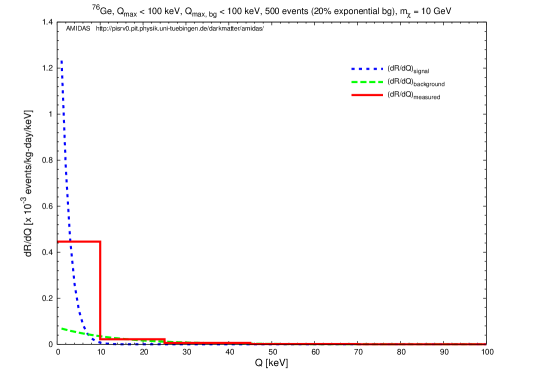
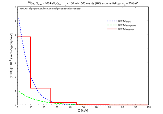
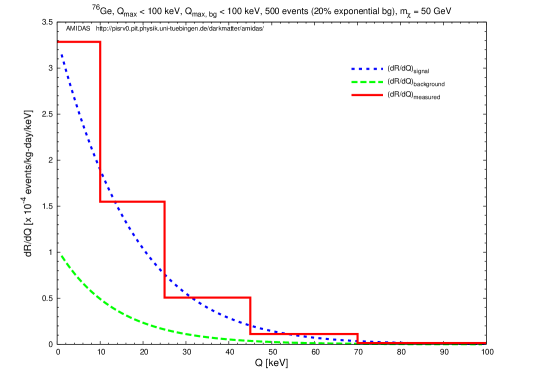
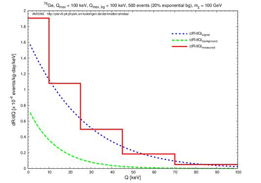
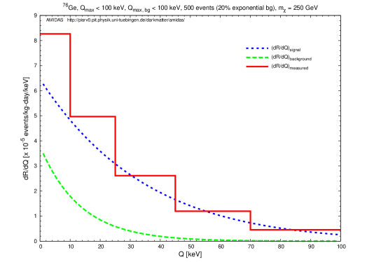
Figure 1: Measured energy spectra (solid red histograms) for a ${}^{76}{\rm Ge}$ target with six different WIMP masses: 10, 25, 50, 100, 250, and 500 GeV. The dotted blue curves are the elastic WIMP–nucleus scattering spectra, whereas the dashed green curves are the exponential background spectra normalized to fit to the chosen background ratio, which has been set as 20% here. The experimental threshold energies have been assumed to be negligible and the maximal cut–off energies are set as 100 keV. The background windows have been assumed to be the same as the experimental possible energy ranges. 5,000 experiments with 500 total events on average in each experiment have been simulated. See the text for further details (plots from Ref. [23]).

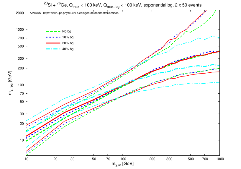
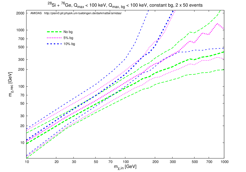
Figure 2: The reconstructed WIMP masses and the lower and upper bounds of the 1$\sigma$ statistical uncertainties by using mixed data sets from WIMP–induced and background events as functions of the input WIMP mass. ${}^{28}{\rm Si}$ and ${}^{76}{\rm Ge}$ have been chosen as two target nuclei. The exponential (upper) and constant (lower) forms given in Eqs. (21) and (20) have been used for the background spectrum. The background ratios shown here are no background (dashed green), 5% (dotted magenta), 10% (long–dotted blue), 20% (solid red), and 40% (dash–dotted cyan) background events in the analyzed data sets in the experimental energy ranges between 0 and 100 keV. Each experiment contains 50 total events on average. Other parameters are as in Figs. 1. See the text for further details (plots from Ref. [23]).

3.1 On the measured energy spectrum

In Figs. 1 I show measured energy spectra (solid red histograms) for a ${}^{76}{\rm Ge}$ target with six different WIMP masses: 10, 25, 50, 100, 250, and 500 GeV based on Monte Carlo simulations. The dotted blue curves are the elastic WIMP–nucleus scattering spectra, whereas the dashed green curves are the exponential background spectra given in Eq. (21), which have been normalized so that the ratios of the areas under these background spectra to those under the (dotted blue) WIMP scattering spectra are equal to the background–signal ratio in the whole data sets (e.g., 20% backgrounds to 80% signals shown in Figs. 1). The experimental threshold energies have been assumed to be negligible and the maximal cut–off energies are set as 100 keV. The background windows (the possible energy ranges in which residue background events exist) have been assumed to be the same as the experimental possible energy ranges. 5,000 experiments with 500 total events on average in each experiment have been simulated.

Remind that the measured energy spectra shown here are averaged over the simulated experiments. Five bins with linear increased bin widths have been used for binning generated signal and background events. As argued in Ref. [12], for reconstructing the one–dimensional WIMP velocity distribution function, this unusual, particular binning has been chosen in order to accumulate more events in high energy ranges and thus to reduce the statistical uncertainties in high velocity ranges. However, as shown in Sec. 2, for the estimation of the SI WIMP–nucleon coupling (as well as for the determination of the WIMP mass [6]), one needs either events in the first energy bin or all events in the whole data set. Hence, there is in practice no difference between using an equal bin width for all bins or a (linear) increased bin widths.

It can be found in Figs. 1 that the shape of the WIMP scattering spectrum depends highly on the WIMP mass: for light WIMPs ($m_{\chi}~{}\>\raisebox{-3.01385pt}{$\stackrel{{\scriptstyle\textstyle<}}{{\sim}}$}\>~{}50$ GeV), the recoil spectra drop sharply with increasing recoil energies, while for heavy WIMPs ($m_{\chi}~{}\>\raisebox{-3.01385pt}{$\stackrel{{\scriptstyle\textstyle>}}{{\sim}}$}\>~{}100$ GeV), the spectra become flatter. In contrast, the exponential background spectra shown here depend only on the target mass and are rather flatter (sharper) for light (heavy) WIMP masses compared to the WIMP scattering spectra. This means that, once input WIMPs are light (heavy), background events would contribute relatively more to high (low) energy ranges, and, consequently, the measured energy spectra would mimic scattering spectra induced by heavier (lighter) WIMPs. Moreover, for heavy WIMP masses, since background events would contribute relatively more to low energy ranges, the estimated value of the measured recoil spectrum at the lowest experimental cut–off energy, $r(Q_{\rm min})$, could thus be (strongly) overestimated.

More detailed illustrations and discussions about the effects of residue background events on the measured energy spectrum can be found in Ref. [23].

3.2 On the reconstructed WIMP mass

Figs. 2 show the reconstructed WIMP masses and the lower and upper bounds of the 1$\sigma$ statistical uncertainties by means of the model–independent procedure introduced in Refs. [5, 6] with mixed data sets from WIMP–induced and background events as functions of the input WIMP mass. As in Ref. [6], ${}^{28}{\rm Si}$ and ${}^{76}{\rm Ge}$ have been chosen as two target nuclei. The experimental threshold energies of two experiments have been assumed to be negligible and the maximal cut–off energies are set the same as 100 keV. The exponential (upper) and constant (lower) forms given in Eqs. (21) and (20) have been used for the background spectrum. The background windows are set the same as the experimental possible energy ranges for both experiments. The background ratios shown here are no background (dashed green), 5% (dotted magenta), 10% (long–dotted blue), 20% (solid red), and 40% (dash–dotted cyan) background events in the analyzed data sets. 2 $\times$ 5,000 experiments have been simulated. Each experiment contains 50 total events on average. Note that all events recorded in our data sets are treated as WIMP signals in the analysis, although statistically we know that a fraction of these events could be backgrounds.

From the upper frame of Figs. 2 it can be seen clearly that, for light WIMP masses ($m_{\chi}~{}\>\raisebox{-3.01385pt}{$\stackrel{{\scriptstyle\textstyle<}}{{\sim}}$}\>~{}100$ GeV), caused by the relatively flatter background spectrum (compared to the scattering spectrum induced by light WIMPs), the energy spectrum of all recorded events would mimic a scattering spectrum induced by WIMPs with a relatively heavier mass, and, consequently, the reconstructed WIMP masses as well as the statistical uncertainty intervals could be overestimated. In contrast, for heavy WIMP masses ($m_{\chi}~{}\>\raisebox{-3.01385pt}{$\stackrel{{\scriptstyle\textstyle>}}{{\sim}}$}\>~{}100$ GeV), caused by the relatively sharper background spectrum, relatively more background events contribute to low energy ranges, and the energy spectrum of all recorded events would mimic a scattering spectrum induced by WIMPs with a relatively lighter mass. Hence, the reconstructed WIMP masses as well as the statistical uncertainty intervals could be underestimated.

As a comparison, the lower frame of Figs. 2 shows that, since the constant background spectrum is flatter for all WIMP masses, background events contribute always relatively more to high energy ranges, and the measured energy spectra would thus always mimic scattering spectra induced by heavier WIMPs. Therefore, the reconstructed WIMP masses as well as the statistical uncertainty intervals are overestimated for all input WIMP masses.

Moreover, Figs. 2 show that the larger the fraction of background events in the analyzed data sets, the more strongly over-/underestimated the reconstructed WIMP masses as well as the statistical uncertainty intervals. Nevertheless, it can be found that, with $\sim$ 10% – 20% residue background events in the analyzed data sets of $\sim$ 50 total events, the 1$\sigma$ statistical uncertainty band could in principle cover the true WIMP mass pretty well.

More detailed illustrations and discussions about the effects of residue background events on the determination of the WIMP mass can be found in Ref. [23].

4 Results of the reconstructed SI WIMP–nucleon coupling

In this section I present simulation results of the reconstructed SI WIMP coupling on nucleons by means of the model–independent method described in Sec. 2 with mixed data sets from WIMP–induced and background events. The WIMP mass $m_{\chi}$ appearing in the expression (13) for estimating $|f_{\rm p}|^{2}$ has been assumed to be known precisely from other (e.g., collider) experiments with an overall uncertainty of 5% of the input (true) WIMP mass or determined from other two direct detection experiments. The SI WIMP–nucleon cross section for our simulations is set as $\sigma_{\chi{\rm p}}^{\rm SI}=10^{-8}$ pb, the currently most commonly used value for the local WIMP density, $\rho_{0}=0.3~{}{\rm GeV/cm^{3}}$, needed in Eq. (13) has been used for both simulations and data analyses. A ${}^{76}{\rm Ge}$ nucleus has been chosen as our detector target for reconstructing $|f_{\rm p}|^{2}$, whereas a ${}^{28}{\rm Si}$ target and a second ${}^{76}{\rm Ge}$ target have been used for determining $m_{\chi}$. The experimental threshold energies of all experiments have been assumed to be negligible and the maximal cut–off energies are set the same as 100 keV. The exponential background spectrum given in Eq. (21) has been used for generating background events in windows of the entire experimental possible ranges. (3 $\times$) 5,000 experiments have been simulated.

Fig. 3 shows the reconstructed squared SI WIMP–nucleon couplings, $|f_{\rm p}|^{2}$, and their lower and upper bounds of the 1$\sigma$ statistical uncertainties by using mixed data sets as functions of the input WIMP mass. The WIMP mass $m_{\chi}$ needed in Eq. (13) has been assumed to be known precisely. The background ratios shown here are no background (dashed green), 10% (long–dotted blue), 20% (solid red), and 40% (dash–dotted cyan) background events in the analyzed data sets in the experimental energy ranges between 0 and 100 keV. Each experiment contains 50 total events on average. Remind that all events recorded in our data sets are treated as WIMP signals in the analysis.

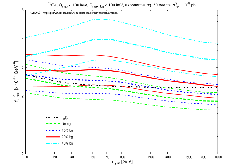
Figure 3: The reconstructed squared SI WIMP–nucleon couplings and the lower and upper bounds of the 1$\sigma$ statistical uncertainties by using mixed data sets from WIMP–induced and background events as functions of the input WIMP mass. A ${}^{76}{\rm Ge}$ nucleus has been chosen as the target. The WIMP mass $m_{\chi}$ needed in Eq. (13) has been assumed to be known precisely. The background ratios shown here are no background (dashed green), 10% (long–dotted blue), 20% (solid red), and 40% (dash–dotted cyan) background events in the analyzed data sets in the experimental energy ranges between 0 and 100 keV. The double–dotted black curve indicates the theoretical value of $|f_{\rm p}|^{2}$ corresponding to the fixed SI WIMP–nucleon cross section $\sigma_{\chi{\rm p}}^{\rm SI}=10^{-8}$ pb. Each data set contains 50 total events on average. Other parameters are as in Figs. 1. See the text for further details.

It can be found in Fig. 3 that the larger the background ratio in the analyzed data set, the more strongly overestimated the reconstructed SI WIMP–nucleon coupling for all input WIMP masses. This can be understood from the expression (1) for the different event rate $dR/dQ$. For a given WIMP mass and a specified target nucleus, the SI WIMP–nucleus cross section is proportional to the total event number–to–exposure ratio:

$$\sigma_{0}^{\rm SI}\simeq\left(\frac{4}{\pi}\right)m_{\rm r,N}^{2}A^{2}|f_{\rm p}|^{2}\propto\frac{1}{{\cal E}}\int_{Q_{\rm min}}^{Q_{\rm max}}\left(\frac{dR}{dQ}\right)_{\rm expt}dQ=\frac{R_{\rm expt}(Q_{\rm min},Q_{\rm max})}{{\cal E}_{\rm sg}}~{}\!.$$ (22)

Here and throughout the subscripts “sg” and “bg” stand for WIMP signals and background events, respectively; ${\cal E}_{\rm sg}$ is the required exposure to observe the expected “WIMP signal” (not total) events. Note that, since background events in our data set are in fact unexpected, the exposure ${\cal E}$ in Eqs. (12) and (13) should thus be equal to ${\cal E}_{\rm sg}$. For a fixed number of total “observed” events, the larger the background ratio, or, equivalently, the smaller the number of real WIMP–induced events, the smaller the required exposure ${\cal E}={\cal E}_{\rm sg}$ for accumulating the total observed events, and, therefore, the larger the estimated SI WIMP–nucleon coupling. In other words, due to extra unexpected background events in our data set, one will use a larger number of total events to estimate the SI WIMP coupling, and thus overestimate it.

More exactly (and mathematically), we can separate the prefactor in the second bracket on the right–hand side of Eq. (13) into two terms:

$$\frac{1}{{\cal E}}\!\left[\frac{2Q_{\rm min}^{1/2}r(Q_{\rm min})}{F^{2}(Q_{\rm min})}+I_{0}\!\right]=\frac{1}{{\cal E}_{\rm sg}}\!\left[\frac{2Q_{\rm min}^{1/2}r_{\rm sg}(Q_{\rm min})}{F^{2}(Q_{\rm min})}+I_{0,\rm sg}\!\right]+\frac{1}{{\cal E}_{\rm sg}}\!\left[\frac{2Q_{\rm min}^{1/2}r_{\rm bg}(Q_{\rm min})}{F^{2}(Q_{\rm min})}+I_{0,\rm bg}\!\right].$$ (23)

It can thus be seen clearly that the prefactor in the expression (13) for estimating $|f_{\rm p}|^{2}$ would always be overestimated with non–negligible background events. Remind that $r(Q_{\rm min})$ and $I_{0}$ given in Eqs. (10) and (11) are estimated from the measured recoil spectrum $(dR/dQ)_{\rm expt}$ before normalized by ${\cal E}$ (or, equivalently, ${\cal E}_{\rm sg}$). Hence, while the first term on the right–hand side of Eq. (23) remains unchanged by increasing the background ratio (and in turn with a decreased number of WIMP–induced events), the second term above contributed from residue background events causes the overestimate of the reconstructed SI WIMP coupling. Remind also that the experimental minimal cut–off energy, $Q_{\rm min}$, has been set to be negligible. Thus the first term involving $Q_{\rm min}^{1/2}r_{\rm bg}(Q_{\rm min})$ in the bracket of the second term above does not contribute to the reconstructed $|f_{\rm p}|^{2}$ in our simulations shown here; otherwise, the reconstructed $|f_{\rm p}|^{2}$ could be more strongly overestimated, especially for WIMP masses $m_{\chi}~{}\>\raisebox{-3.01385pt}{$\stackrel{{\scriptstyle\textstyle>}}{{\sim}}$}\>~{}50$ GeV (see Figs. 1).

Moreover, for three cases with background ratios  $\stackrel{{\scriptstyle\textstyle<}}{{\sim}}$  20% shown in Fig. 3, the larger the input WIMP mass, the more strongly overestimated the SI WIMP coupling. However, interestingly, once the background ratio rises to  $\stackrel{{\scriptstyle\textstyle>}}{{\sim}}$  20% (the dash–dotted cyan curves indicate a background ration of 40%), a hump at an input WIMP mass of $\sim$ 60 GeV appears. The reason is as follows. In the appendix I will show that the second term on the right–hand side of Eq. (23) is proportional to the “WIMP scattering” spectrum (not the “background” spectrum!):

$$\frac{1}{{\cal E}_{\rm sg}}\left[\frac{2Q_{\rm min}^{1/2}r_{\rm bg}(Q_{\rm min})}{F^{2}(Q_{\rm min})}+I_{0,\rm bg}\right] \propto \frac{r_{\rm bg}}{1-r_{\rm bg}}\int_{Q_{\rm min}}^{Q_{\rm max}}\left(\frac{dR}{dQ}\right)_{\rm sg}dQ$$ (24)

$$\equiv \left(\frac{r_{\rm bg}}{1-r_{\rm bg}}\right)R_{\rm sg}(Q_{\rm min},Q_{\rm max})~{}\!.$$

Here $(dR/dQ)_{\rm sg}$ and $R_{\rm sg}$ are the normalized differential and total event rate of WIMP signals, respectively; $r_{\rm bg}$ is the ratio of residue background events in the whole data set. It can be understood from Eq. (1) that $(dR/dQ)_{\rm sg}$ and therefore $R_{\rm sg}$ are functions of the input (true) WIMP mass, through not only $m_{\chi}$ and $m_{\rm r,N}$ in the denominator of ${\cal A}$ defined in Eq. (2), but also the transformation constant $\alpha$ in Eq. (5).

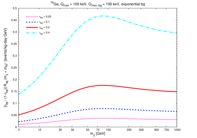
Figure 4: The products of $\big{[}r_{\rm bg}/(1-r_{\rm bg})\big{]}~{}\!R_{\rm sg}$ and $(m_{\chi}+m_{\rm N})$ as functions of $m_{\chi}$ for a ${}^{76}{\rm Ge}$ target with different background ratios $r_{\rm bg}$. The background ratios shown here are 5% (dotted magenta), 10% (long–dotted blue), 20% (solid red), and 40% (dash–dotted cyan). Parameters are as in Fig. 3. See the text for further details.

Fig. 4 shows the products of $\big{[}r_{\rm bg}/(1-r_{\rm bg})\big{]}~{}\!R_{\rm sg}$ and $(m_{\chi}+m_{\rm N})$ as functions of $m_{\chi}$ for a ${}^{76}{\rm Ge}$ target with different background ratios $r_{\rm bg}$. It can be found that the extra contribution from residue background events, which is proportional to the product of $\big{[}r_{\rm bg}/(1-r_{\rm bg})\big{]}~{}\!R_{\rm sg}$ and $(m_{\chi}+m_{\rm N})$, has indeed a maximum at a WIMP mass of $\sim$ 75 GeV. Considering the slightly decreased $|f_{\rm p}|^{2}$ value by increasing the input WIMP mass without background events (the dashed green curves in Fig. 3), the total recorded events (including WIMP–induced and background events) should thus result in a hump of the reconstructed $|f_{\rm p}|^{2}$ at an input WIMP mass of $\sim$ 60 GeV, once the background fraction in our data set is large enough.

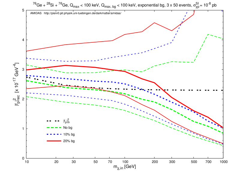
Figure 5: As in Fig. 3, except that the WIMP mass $m_{\chi}$ in Eq. (13) has been reconstructed by using two other data sets with a ${}^{28}{\rm Si}$ target and a second ${}^{76}{\rm Ge}$ target.

In Fig. 5 the WIMP mass $m_{\chi}$ needed in expression (13) has been reconstructed by using two other data sets with a ${}^{28}{\rm Si}$ target and a second ${}^{76}{\rm Ge}$ target. As shown in Figs. 2 and discussed in Sec. 3.2, due to the contribution from residue background events, if the input WIMP mass is light (heavy), the reconstructed mass would be overestimated (underestimated). Hence, for input masses  $\stackrel{{\scriptstyle\textstyle<}}{{\sim}}$  ( $\stackrel{{\scriptstyle\textstyle>}}{{\sim}}$ ) 150 GeV, the SI WIMP–nucleon couplings reconstructed by using three independent data sets would be larger (smaller) than those reconstructed by using only one data set with an extra information about the WIMP mass (cf. Fig. 3). In addition, the statistical uncertainties on the reconstructed SI WIMP couplings would also be (much) larger. However, both Figs. 3 and 5 indicate that one could in principle estimate the SI WIMP–nucleon coupling up to a WIMP mass of $\sim$ 1 TeV by using one or three independent data sets with maximal 20% background events (solid red). For a WIMP mass of 100 GeV and 20% residue background events, the systematic deviation of the reconstructed SI WIMP coupling $|f_{\rm p}|$ (with a reconstructed WIMP mass) would in principle be $\sim+13\%$ with a statistical uncertainty of $\sim^{+21\%}_{-14\%}$ ($\sim-3.3\%^{+18\%}_{-13\%}$ for background–free data sets).

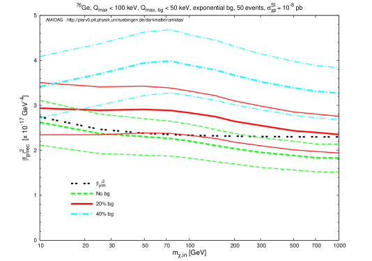
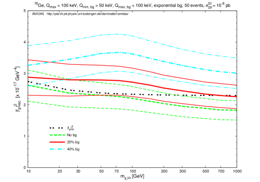
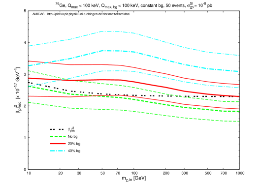
Figure 6: As in Fig. 3, except that the background spectra and/or windows are different: exponential spectrum between 0 and 50 keV (top), exponential spectrum between 50 and 100 keV (middle), and constant spectrum between 0 and 100 keV (bottom).

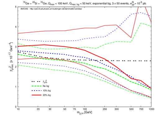
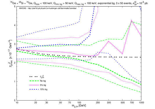
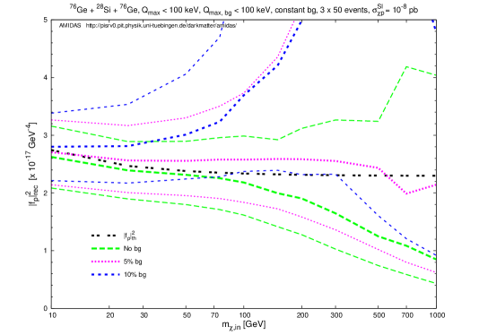
Figure 7: As in Figs. 6, except that the WIMP mass $m_{\chi}$ in Eq. (13) has been reconstructed by using two other data sets with a ${}^{28}{\rm Si}$ target and a second ${}^{76}{\rm Ge}$ target. The background ratios shown in two lower frames are no background (dashed green), 5% (dotted magenta), and 10% (long–dotted blue).

Furthermore, in order to check effects of different background discrimination ability in different energy ranges and the need of a prior knowledge about an (exact) form of the residue background spectrum, in Figs. 6 and 7 we consider two different background windows: between 0 and 50 keV and between 50 and 100 keV for the exponential background spectrum as well as the rather extrem constant spectrum given in Eq. (20) with a window between 0 and 100 keV.

Firstly, from Figs. 6, it can be seen clearly that, by using one data set with up to 20% background events and a precisely known WIMP mass as an input information, the SI WIMP–nucleon coupling $|f_{\rm p}|$ can in principle be estimated with a maximal $\sim+11\%$ systematic deviation (for an input WIMP mass of 100 GeV) from the theoretical value and a statistical uncertainty of $\sim\pm 9\%$. More importantly, all three cases show almost the same result. This indicates that, once the WIMP mass can be known (pretty) precisely, not the exact form of the residue background spectrum, but the amount in the analyzed data set could affect (significantly) the reconstructed SI WIMP–nucleon coupling.

In contrast, results shown in Figs. 7 depend strongly on the reconstruction of the WIMP mass. As discussed in Ref. [23] and Sec. 3.2, for cases with the exponential background spectrum and background windows in the whole experimental possible and low energy ranges, the reconstructed WIMP mass could be slightly overestimated (underestimated), once incident WIMPs are light (heavy). However, for the case with the exponential spectrum and windows in high energy ranges, or the case with the constant spectrum and windows of whole experimental possible energy ranges, the reconstructed WIMP mass could be (strongly) overestimated for all input WIMP masses. Here the effect of a (strongly) overestimated WIMP mass can be seen clearly here. Since for the case shown in Fig. 5 our background spectra are exponential, only very few background events could be observed in the energy range between 50 and 100 keV. Hence, for the case with background windows only in the low energy ranges (top in Figs. 7), not surprisingly, the result of the reconstructed SI WIMP coupling is almost the same as shown in Fig. 5.

However, for the case with the exponential background spectrum and background windows in high energy ranges (middle in Figs. 7) or the case with the constant spectrum in whole experimental possible energy ranges (bottom), the results are almost the same: the larger the background ratio, the more strongly overestimated the SI WIMP coupling, in particular for heavy input WIMP masses. Nevertheless, by using (two or) three data sets with background ratios of $\>\raisebox{-3.01385pt}{$\stackrel{{\scriptstyle\textstyle<}}{{\sim}}$}\>~{}10\%$, one could in principle reconstruct the SI WIMP–nucleon coupling (as well as the WIMP mass [23]) pretty well, without knowing the (exact) form of the background spectrum.

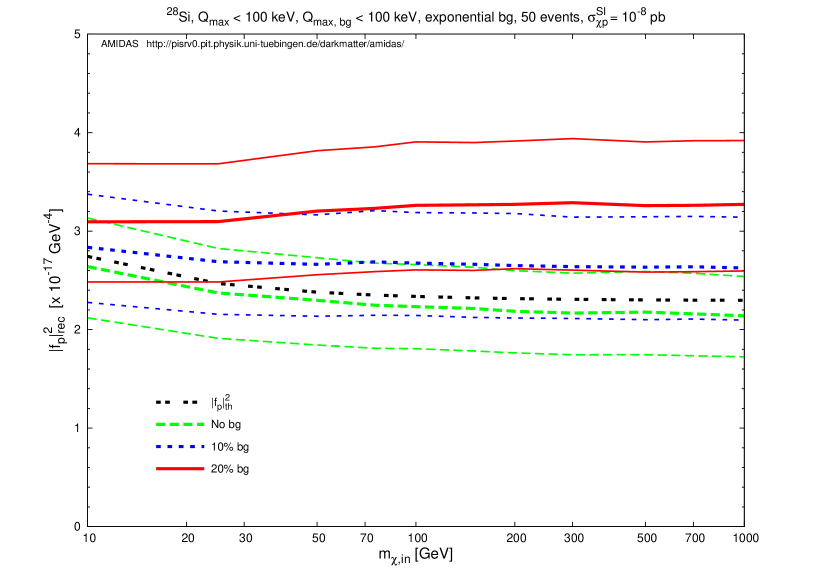
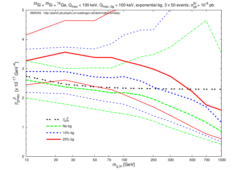
Figure 8: As in Figs. 3 (upper) and 5 (lower), except that ${}^{28}{\rm Si}$ has been used as the (first) target for reconstructing $f_{\rm p}|^{2}$. Remind that two data sets with the ${}^{28}{\rm Si}$ target are different.

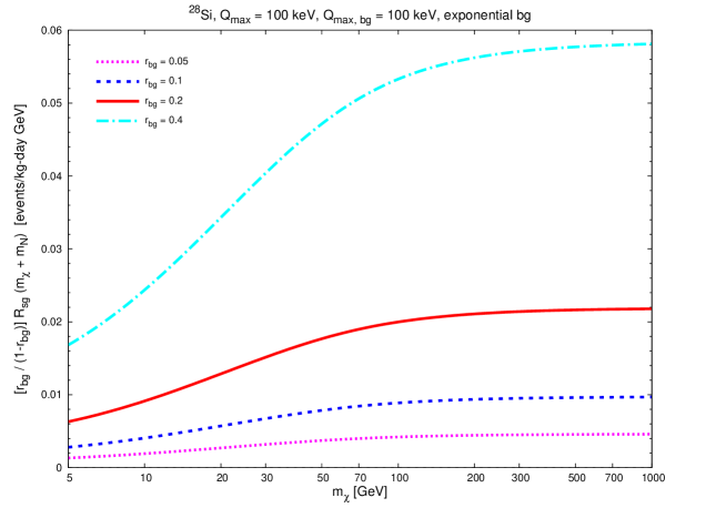
Figure 9: As in Fig. 4, except that a ${}^{28}{\rm Si}$ target has been used.

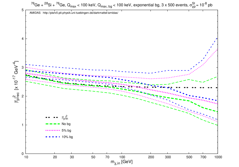
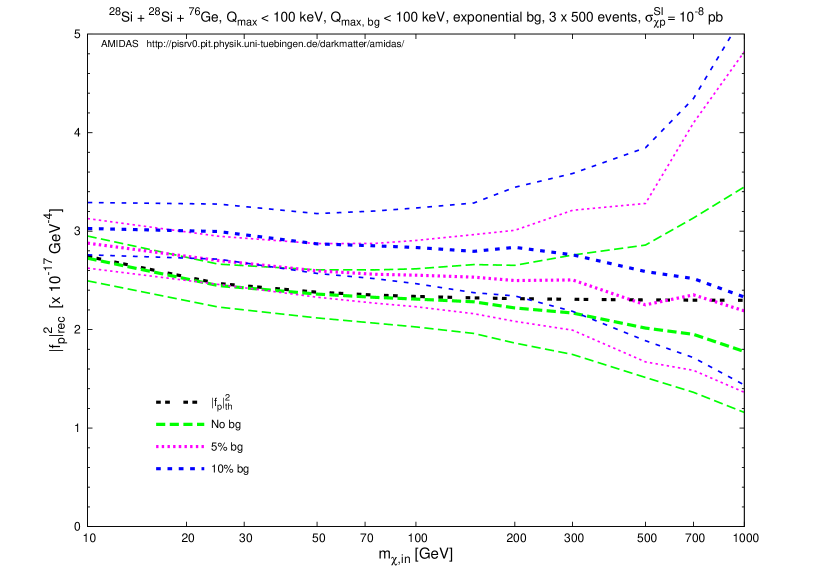
Figure 10: As in Fig. 5 and the lower frame of Figs. 8, except that the expected number of total events in each data set has been risen by a factor of 10, i.e., 500 events on average, for both the ${}^{76}{\rm Ge}$ (upper) and the ${}^{28}{\rm Si}$ (lower) target. The background ratios shown here are no background (dashed green), 5% (dotted magenta), and 10% (long–dotted blue) background events in the analyzed data sets in the experimental energy ranges between 0 and 100 keV.

In Figs. 8 we consider a rather light target nucleus: ${}^{28}{\rm Si}$. The WIMP mass $m_{\chi}$ has been assumed to be known precisely (upper) or reconstructed from other two data sets (lower). Only the exponential form for residue background spectrum has been considered here. Remind that, as found in Refs. [7, 8], with a light target nucleus, e.g., Si or Ar, the statistical uncertainty on the reconstructed SI WIMP–nucleon coupling is larger than that with a heavy nucleus, e.g., Ge or Xe. Consequently, for both cases (with a precisely known or a reconstructed WIMP mass), the reconstructed SI WIMP couplings as well as the 1$\sigma$ statistical uncertainties shown in Figs. 8 are larger than those with ${}^{76}{\rm Ge}$ shown in Figs. 3 and 5.

On the other hand, the systematic deviations of the (under)estimated SI WIMP coupling for heavy input WIMP masses ($m_{\chi}~{}\>\raisebox{-3.01385pt}{$\stackrel{{\scriptstyle\textstyle>}}{{\sim}}$}\>~{}300$ GeV) are smaller for light nuclei than those for heavy ones [7, 8]. In addition, as shown in Fig. 9, the background contribution (the second term on the right–hand side of Eq. (23)) increases pretty quickly with an increased WIMP mass. Hence, for input WIMP masses $m_{\chi}~{}\>\raisebox{-3.01385pt}{$\stackrel{{\scriptstyle\textstyle>}}{{\sim}}$}\>~{}100$ GeV, the reconstructed SI WIMP–nucleon couplings with a ${}^{28}{\rm Si}$ target nucleus would be more strongly overestimated than those reconstructed with a ${}^{76}{\rm Ge}$ target. Nevertheless, for both cases (with a precisely known or a reconstructed WIMP mass), with $\sim$ 10% – 20% background events in our data sets, the 1$\sigma$ statistical uncertainty bands could in principle still cover the theoretical value of $|f_{\rm p}|$. For an input WIMP mass of 100 GeV, by using three data sets with 10% background events, the systematic deviation of and the statistical uncertainty on the reconstructed SI WIMP–nucleon coupling $|f_{\rm p}|$ is $\sim+8\%^{+26\%}_{-17\%}$ ($\sim-3\%^{+23\%}_{-17\%}$ for background–free data sets).

Finally, considering the progress of detection and background discrimination techniques of the next–generation ton–scale detectors, in Figs. 10 we rise the expected number of total events in each data set by a factor of 10, i.e., 500 events on average, for both ${}^{76}{\rm Ge}$ (upper) and ${}^{28}{\rm Si}$ (lower) targets. Here I show only the results with the reconstructed WIMP mass. Since the statistical uncertainties shrink now by a factor of $\>\raisebox{-3.01385pt}{$\stackrel{{\scriptstyle\textstyle>}}{{\sim}}$}\>~{}3$, the maximal acceptable background ratio becomes $\sim$ 5% (i.e., $\sim$ 25 residue background events in each data set). For an input WIMP mass of 100 GeV, the systematic deviation would then be $\sim+2\%$ (with Ge) and $\sim+5\%$ (with Si) with a statistical uncertainty of $\sim 5\%$ (with Ge) and $\sim 7\%$ (with Si).

5 Summary and conclusions

In this paper I reexamine the model–independent data analysis method introduced in Refs. [7, 8] for the estimation of the spin–independent scalar coupling of Weakly Interacting Massive Particles on nucleons from data (measured recoil energies) of direct Dark Matter detection experiments directly by taking into account a fraction of residue background events, which pass all discrimination criteria and then mix with other real WIMP–induced events in the analyzed data sets. This method requires neither prior knowledge about the WIMP scattering spectrum nor about different possible background spectra; the needed information is the recoil energies recorded in direct detection experiments, an unique assumption about the local WIMP density, and (occasionally) the mass of incident WIMPs.

For the mass of incident WIMPs required in this data analysis, we considered two cases: known precisely with an overall uncertainty (of 5% of the input WIMP mass in our simulations) from other (e.g., collider) experiments as well as reconstructed by using other direct detection experiments. Our simulations show that, assuming an exponential form for the residue background spectrum, with $\sim$ 50 total events in each data set, for both cases the maximal acceptable background ratio is $\sim$ 20% (i.e., $\sim$ 10 background events). For a WIMP mass of 100 GeV and 20% residue background events, the systematic deviation of the reconstructed SI WIMP coupling $|f_{\rm p}|$ (with a reconstructed WIMP mass) would in principle be $\sim+13\%$ with a statistical uncertainty of $\sim^{+21\%}_{-14\%}$ ($\sim-3.3\%^{+18\%}_{-13\%}$ for background–free data sets).

Furthermore, in order to check effects of different background discrimination ability in different energy ranges and the need of a prior knowledge about an (exact) form of the residue background spectrum, we considered two different background windows: between 0 and 50 keV and between 50 and 100 keV for the exponential background spectrum as well as the rather extrem constant spectrum with a window between 0 and 100 keV. It has been found that, with a precisely known WIMP mass, all three cases show almost the same result as that for the exponential background spectrum with a window of the whole experimental possible energy range. This indicates that, once the WIMP mass can be known (pretty) precisely, not the exact form of the residue background spectrum, but their amount in the analyzed data set could affect (significantly) the reconstructed SI WIMP–nucleon coupling.

On the other hand, we considered a rather light target nucleus: ${}^{28}{\rm Si}$ with both a precisely known and a reconstructed WIMP mass. For both cases the reconstructed SI WIMP couplings would be more strongly overestimated and the 1$\sigma$ statistical uncertainties would also be larger than those with ${}^{76}{\rm Ge}$. Nevertheless, with $\sim$ 10% – 20% background events in our data sets, the 1$\sigma$ statistical uncertainty bands could in principle still cover the theoretical value of $|f_{\rm p}|$. For an input WIMP mass of 100 GeV, by using three data sets with 10% background events, the systematic deviation of and the statistical uncertainty on the reconstructed SI WIMP–nucleon coupling $|f_{\rm p}|$ is $\sim+8\%^{+26\%}_{-17\%}$ ($\sim-3\%^{+23\%}_{-17\%}$ for background–free data sets).

Finally, for rather next–generation ton–scale detectors, we considered the use of data sets of ${\cal O}(500)$ events for both ${}^{76}{\rm Ge}$ and ${}^{28}{\rm Si}$ targets. Our results show that, with a maximal background ratio of 5% (i.e., $\sim$ 25 total events in each data set), one could in principle still reconstructed the SI WIMP–nucleon coupling pretty well: for an input WIMP mass of 100 GeV, the systematic deviation would be $\sim+2\%$ (with Ge) and $\sim+5\%$ (with Si) with a statistical uncertainty of $\sim 5\%$ (with Ge) and $\sim 7\%$ (with Si).

In summary, as the third part of the study of the effects of residue background events in direct Dark Matter detection experiments, we considered the estimation of the SI WIMP–nucleon coupling. Our results show that, with currently running and projected experiments using detectors with $10^{-9}$ to $10^{-11}$ pb sensitivities [29, 20, 30, 31] and $<10^{-6}$ background rejection ability [19, 21, 22, 18], once one or more experiments with different target nuclei could accumulate a few tens events (in one experiment), we could in principle already estimate the SI coupling of Dark Matter particles on ordinary matter with a reasonable precession, or at least give an upper bound on that, even though there could be some background events mixed in our data sets for the analysis and the reconstructed value would thus be overestimated. Moreover, although two forms for background spectrum and three windows for residue background events considered in this work are rather naive; one should be able to extend our observations/discussions to predict the effects of possible background events in their own experiment. Hopefully, this will encourage our experimental colleagues to present their (future) results as the “most possible area(s)” in the parameter space of different extensions of the Standard Model of particle physics and in turn to offer stringenter information for identifying (WIMP) Dark Matter particles at colliders as well as for predicting spectra in indirect Dark Matter detection experiments.

Acknowledgments

The author would like to thank the Physikalisches Institut der Universität Tübingen for the technical support of the computational work demonstrated in this article. This work was partially supported by the National Science Council of R.O.C. under contract no. NSC-99-2811-M-006-031 as well as by the LHC Physics Focus Group, National Center of Theoretical Sciences, R.O.C..

Appendix A Formulae needed in Sec. 2

Here I list all formulae needed for the model–independent data analysis procedure used in Sec. 2. Detailed derivations and discussions can be found in Refs. [12, 6].

A.1 Estimating $r(Q_{\rm min})$ and $I_{n}(Q_{\rm min},Q_{\rm max})$

First, consider experimental data described by

$${\textstyle Q_{n}-\frac{b_{n}}{2}}\leq Q_{n,i}\leq{\textstyle Q_{n}+\frac{b_{n}}{2}}~{}\!,~{}~{}~{}~{}~{}~{}~{}~{}~{}~{}~{}~{}i=1,~{}2,~{}\cdots,~{}N_{n},~{}n=1,~{}2,~{}\cdots,~{}B.$$ (A1)

Here the total energy range between $Q_{\rm min}$ and $Q_{\rm max}$ has been divided into $B$ bins with central points $Q_{n}$ and widths $b_{n}$. In each bin, $N_{n}$ events will be recorded. Since the recoil spectrum $dR/dQ$ is expected to be approximately exponential, the following ansatz for the measured recoil spectrum (before normalized by the experimental exposure ${\cal E}$) in the $n$th bin has been introduced [12]:

$$\left(\frac{dR}{dQ}\right)_{{\rm expt},~{}\!n}\equiv\left(\frac{dR}{dQ}\right)_{{\rm expt},~{}\!Q\simeq Q_{n}}\equiv r_{n}~{}\!e^{k_{n}(Q-Q_{s,n})}~{}\!.$$ (A2)

Here $r_{n}$ is the standard estimator for $(dR/dQ)_{\rm expt}$ at $Q=Q_{n}$:

$$r_{n}=\frac{N_{n}}{b_{n}}~{}\!,$$ (A3)

$k_{n}$ is the logarithmic slope of the recoil spectrum in the $n$th $Q-$bin, which can be computed numerically from the average value of the measured recoil energies in this bin:

$$\overline{Q-Q_{n}}|_{n}=\left(\frac{b_{n}}{2}\right)\coth\left(\frac{k_{n}b_{n}}{2}\right)-\frac{1}{k_{n}}~{}\!,$$ (A4)

where

$$\overline{(Q-Q_{n})^{\lambda}}|_{n}\equiv\frac{1}{N_{n}}\sum_{i=1}^{N_{n}}\left(Q_{n,i}-Q_{n}\right)^{\lambda}~{}\!.$$ (A5)

The error on the logarithmic slope $k_{n}$ can be estimated from Eq. (A4) directly as

$$\sigma^{2}(k_{n})=k_{n}^{4}\left\{1-\left[\frac{k_{n}b_{n}/2}{\sinh(k_{n}b_{n}/2)}\right]^{2}\right\}^{-2}\sigma^{2}\left(\overline{Q-Q_{n}}|_{n}\right)~{}\!,$$ (A6)

with

$$\sigma^{2}\left(\overline{Q-Q_{n}}|_{n}\right)=\frac{1}{N_{n}-1}\bigg{[}\overline{(Q-Q_{n})^{2}}|_{n}-\overline{Q-Q_{n}}|_{n}^{2}\bigg{]}~{}\!.$$ (A7)

$Q_{s,n}$ in the ansatz (A2) is the shifted point at which the leading systematic error due to the ansatz is minimal [12],

$$Q_{s,n}=Q_{n}+\frac{1}{k_{n}}\ln\left[\frac{\sinh(k_{n}b_{n}/2)}{k_{n}b_{n}/2}\right]~{}\!.$$ (A8)

Note that $Q_{s,n}$ differs from the central point of the $n$th bin, $Q_{n}$. From the ansatz (A2), the counting rate at $Q=Q_{\rm min}$ can be calculated by

$$r(Q_{\rm min})=r_{1}e^{k_{1}(Q_{\rm min}-Q_{s,1})}~{}\!,$$ (A9)

and its statistical error can be expressed as

$$\sigma^{2}(r(Q_{\rm min}))=r^{2}(Q_{\rm min})\left\{\frac{1}{N_{1}}+\left[\frac{1}{k_{1}}-\left(\frac{b_{1}}{2}\right)\left(1+\coth\left(\frac{b_{1}k_{1}}{2}\right)\right)\right]^{2}\sigma^{2}(k_{1})\right\}~{}\!,$$ (A10)

since

$$\sigma^{2}(r_{n})=\frac{N_{n}}{b_{n}^{2}}~{}\!.$$ (A11)

Finally, since all $I_{n}$ are determined from the same data, they are correlated with

$${\rm cov}(I_{n},I_{m})=\sum_{a=1}^{N_{\rm tot}}\frac{Q_{a}^{(n+m-2)/2}}{F^{4}(Q_{a})}~{}\!,$$ (A12)

where the sum runs over all events with recoil energy between $Q_{\rm min}$ and $Q_{\rm max}$. And the correlation between the errors on $r(Q_{\rm min})$, which is calculated entirely from the events in the first bin, and on $I_{n}$ is given by

$${\rm cov}(r(Q_{\rm min}),I_{n})$$ (A13)

$$= r(Q_{\rm min})~{}\!I_{n}(Q_{\rm min},Q_{\rm min}+b_{1})$$

$$~{}~{}~{}~{}\times\left\{\frac{1}{N_{1}}+\left[\frac{1}{k_{1}}-\left(\frac{b_{1}}{2}\right)\left(1+\coth\left(\frac{b_{1}k_{1}}{2}\right)\right)\right]\right.$$

$$~{}~{}~{}~{}~{}~{}~{}~{}~{}~{}~{}~{}~{}~{}\times\left.\left[\frac{I_{n+2}(Q_{\rm min},Q_{\rm min}+b_{1})}{I_{n}(Q_{\rm min},Q_{\rm min}+b_{1})}-Q_{1}+\frac{1}{k_{1}}-\left(\frac{b_{1}}{2}\right)\coth\left(\frac{b_{1}k_{1}}{2}\right)\right]\sigma^{2}(k_{1})\right\}~{}\!;$$

note that the sums $I_{i}$ here only count in the first bin, which ends at $Q=Q_{\rm min}+b_{1}$.

On the other hand, with a functional form of the recoil spectrum (e.g., fitted to experimental data), $(dR/dQ)_{\rm expt}$, one can use the following integral forms to replace the summations given above. Firstly, the average $Q-$value in the $n$th bin defined in Eq. (A5) can be calculated by

$$\overline{(Q-Q_{n})^{\lambda}}|_{n}=\frac{1}{N_{n}}\int_{Q_{n}-b_{n}/2}^{Q_{n}+b_{n}/2}\left(Q-Q_{n}\right)^{\lambda}\left(\frac{dR}{dQ}\right)_{\rm expt}dQ~{}\!.$$ (A14)

For $I_{n}(Q_{\rm min},Q_{\rm max})$ given in Eq. (11), we have

$$I_{n}(Q_{\rm min},Q_{\rm max})=\int_{Q_{\rm min}}^{Q_{\rm max}}\frac{Q^{(n-1)/2}}{F^{2}(Q)}\left(\frac{dR}{dQ}\right)_{\rm expt}dQ~{}\!,$$ (A15)

and similarly for the covariance matrix for $I_{n}$ in Eq. (A12),

$${\rm cov}(I_{n},I_{m})=\int_{Q_{\rm min}}^{Q_{\rm max}}\frac{Q^{(n+m-2)/2}}{F^{4}(Q)}\left(\frac{dR}{dQ}\right)_{\rm expt}dQ~{}\!.$$ (A16)

Remind that $(dR/dQ)_{\rm expt}$ is the measured recoil spectrum before normalized by the exposure. Finally, $I_{i}(Q_{\rm min},Q_{\rm min}+b_{1})$ needed in Eq. (A13) can be calculated by

$$I_{n}(Q_{\rm min},Q_{\rm min}+b_{1})=\int_{Q_{\rm min}}^{Q_{\rm min}+b_{1}}\frac{Q^{(n-1)/2}}{F^{2}(Q)}\bigg{[}r_{1}~{}\!e^{k_{1}(Q-Q_{s,1})}\bigg{]}dQ~{}\!.$$ (A17)

Note that, firstly, $r(Q_{\rm min})$ and $I_{n}(Q_{\rm min},Q_{\rm min}+b_{1})$ should be estimated by Eqs. (A9) and (A17) with $r_{1}$, $k_{1}$ and $Q_{s,1}$ estimated by Eqs. (A3), (A4), and (A8) in order to use the other formulae for estimating the (correlations between the) statistical errors without any modification. Secondly, $r(Q_{\rm min})$ and $I_{n}(Q_{\rm min},Q_{\rm max})$ estimated from a scattering spectrum fitted to experimental data are usually not model–independent any more.

A.2 Determining the WIMP mass $m_{\chi}$

By requiring that the values of a given moment of $f_{1}(v)$ estimated by Eq. (9) from two experiments with different target nuclei, $X$ and $Y$, agree, $m_{\chi}$ appearing in the prefactor $\alpha^{n}$ on the right–hand side of Eq. (9) can be solved analytically as [5, 6]:

$$\left.m_{\chi}\right|_{\left<{v^{n}}\right>}=\frac{\sqrt{m_{X}m_{Y}}-m_{X}({\cal R}_{n,X}/{\cal R}_{n,Y})}{{\cal R}_{n,X}/{\cal R}_{n,Y}-\sqrt{m_{X}/m_{Y}}}~{}\!,$$ (A18)

with ${\cal R}_{n,(X,Y)}$ defined by

$${\cal R}_{n,X}\equiv\left[\frac{2Q_{{\rm min},X}^{(n+1)/2}r_{X}(Q_{{\rm min},X})/F_{X}^{2}(Q_{{\rm min},X})+(n+1)I_{n,X}}{2Q_{{\rm min},X}^{1/2}r_{X}(Q_{{\rm min},X})/F_{X}^{2}(Q_{{\rm min},X})+I_{0,X}}\right]^{1/n}~{}\!,$$ (A19)

and ${\cal R}_{n,Y}$ can be defined analogously. Here $n\neq 0$, $m_{(X,Y)}$ and $F_{(X,Y)}(Q)$ are the masses and the form factors of the nucleus $X$ and $Y$, respectively, and $r_{(X,Y)}(Q_{{\rm min},(X,Y)})$ refer to the counting rates for the target $X$ and $Y$ at the respective lowest recoil energies included in the analysis. Note that the general expression (A18) can be used either for spin–independent or for spin–dependent scattering, one only needs to choose different form factors under different assumptions; the form factors needed for estimating $I_{n,(X,Y)}$ by Eq. (11) or (A15) are thus also different.

By using the standard Gaussian error propagation, a lengthy expression for the statistical uncertainty on $\left.m_{\chi}\right|_{\left<{v^{n}}\right>}$ given in Eq. (A18) can be obtained as

$$\left.\sigma(m_{\chi})\right|_{\left<{v^{n}}\right>} = \frac{\sqrt{m_{X}/m_{Y}}\left|m_{X}-m_{Y}\right|\left({\cal R}_{n,X}/{\cal R}_{n,Y}\right)}{\left({\cal R}_{n,X}/{\cal R}_{n,Y}-\sqrt{m_{X}/m_{Y}}\right)^{2}}$$ (A20)

$$~{}~{}~{}~{}\times\left[\frac{1}{{\cal R}_{n,X}^{2}}\sum_{i,j=1}^{3}\left(\frac{\partial{\cal R}_{n,X}}{\partial c_{i,X}}\right)\left(\frac{\partial{\cal R}_{n,X}}{\partial c_{j,X}}\right){\rm cov}(c_{i,X},c_{j,X})+(X\longrightarrow Y)\right]^{1/2}\!.$$

Here a short–hand notation for the six quantities on which the estimate of $m_{\chi}$ depends has been introduced:

$$c_{1,X}=I_{n,X}~{}\!,~{}~{}~{}~{}~{}~{}~{}~{}~{}~{}~{}~{}c_{2,X}=I_{0,X}~{}\!,~{}~{}~{}~{}~{}~{}~{}~{}~{}~{}~{}~{}c_{3,X}=r_{X}(Q_{{\rm min},X})~{}\!;$$ (A21)

and similarly for the $c_{i,Y}$. Estimators for ${\rm cov}(c_{i},c_{j})$ have been given in Eqs. (A12) and (A13). Explicit expressions for the derivatives of ${\cal R}_{n,X}$ with respect to $c_{i,X}$ are:

$$\frac{\partial{\cal R}_{n,X}}{\partial I_{n,X}}=\frac{n+1}{n}\left[\frac{F_{X}^{2}(Q_{{\rm min},X})}{2Q_{{\rm min},X}^{(n+1)/2}r_{X}(Q_{{\rm min},X})+(n+1)I_{n,X}F_{X}^{2}(Q_{{\rm min},X})}\right]{\cal R}_{n,X}~{}\!,$$ (A22a)

$$\frac{\partial{\cal R}_{n,X}}{\partial I_{0,X}}=-\frac{1}{n}\left[\frac{F_{X}^{2}(Q_{{\rm min},X})}{2Q_{{\rm min},X}^{1/2}r_{X}(Q_{{\rm min},X})+I_{0,X}F_{X}^{2}(Q_{{\rm min},X})}\right]{\cal R}_{n,X}~{}\!,$$ (A22b)

and

$$\frac{\partial{\cal R}_{n,X}}{\partial r_{X}(Q_{{\rm min},X})} = \frac{2}{n}\left[\frac{Q_{{\rm min},X}^{(n+1)/2}I_{0,X}-(n+1)Q_{{\rm min},X}^{1/2}I_{n,X}}{2Q_{{\rm min},X}^{(n+1)/2}r_{X}(Q_{{\rm min},X})+(n+1)I_{n,X}F_{X}^{2}(Q_{{\rm min},X})}\right]$$ (A22c)

$$~{}~{}~{}~{}~{}~{}~{}~{}~{}~{}~{}~{}~{}~{}~{}~{}\times\left[\frac{F_{X}^{2}(Q_{{\rm min},X})}{2Q_{{\rm min},X}^{1/2}r_{X}(Q_{{\rm min},X})+I_{0,X}F_{X}^{2}(Q_{{\rm min},X})}\right]{\cal R}_{n,X}~{}\!;$$

explicit expressions for the derivatives of ${\cal R}_{n,Y}$ with respect to $c_{i,Y}$ can be given analogously. Note that, firstly, factors ${\cal R}_{n,(X,Y)}$ appear in all these expressions, which can practically be cancelled by the prefactors in the bracket in Eq. (A20). Secondly, all the $I_{0,(X,Y)}$ and $I_{n,(X,Y)}$ should be understood to be computed according to Eq. (11) or (A15) with integration limits $Q_{\rm min}$ and $Q_{\rm max}$ specific for that target.

On the other hand, since $|f_{\rm p}|^{2}$ in Eq. (13) is identical for different targets, it leads to a second expression for determining $m_{\chi}$ [6]:

$$\left.m_{\chi}\right|_{\sigma}=\frac{\left(m_{X}/m_{Y}\right)^{5/2}m_{Y}-m_{X}({\cal R}_{\sigma,X}/{\cal R}_{\sigma,Y})}{{\cal R}_{\sigma,X}/{\cal R}_{\sigma,Y}-\left(m_{X}/m_{Y}\right)^{5/2}}~{}\!.$$ (A23)

Here $m_{(X,Y)}\propto A_{(X,Y)}$ has been assumed, and ${\cal R}_{\sigma,(X,Y)}$ are defined by

$${\cal R}_{\sigma,X}\equiv\frac{1}{{\cal E}_{X}}\left[\frac{2Q_{{\rm min},X}^{1/2}r_{X}(Q_{{\rm min},X})}{F_{X}^{2}(Q_{{\rm min},X})}+I_{0,X}\right]~{}\!,$$ (A24)

and similarly for ${\cal R}_{\sigma,Y}$; ${\cal E}_{(X,Y)}$ here are the experimental exposures with the target $X$ and $Y$. Similar to the analogy between Eqs. (A18) and (A23), the statistical uncertainty on $\left.m_{\chi}\right|_{\sigma}$ given in Eq. (A23) can be expressed as

$$\left.\sigma(m_{\chi})\right|_{\sigma} = \frac{\left(m_{X}/m_{Y}\right)^{5/2}\left|m_{X}-m_{Y}\right|\left({\cal R}_{\sigma,X}/{\cal R}_{\sigma,Y}\right)}{\left[{\cal R}_{\sigma,X}/{\cal R}_{\sigma,Y}-\left(m_{X}/m_{Y}\right)^{5/2}\right]^{2}}$$ (A25)

$$~{}~{}~{}~{}~{}~{}\times\left[\frac{1}{{\cal R}_{\sigma,X}^{2}}\sum_{i,j=2}^{3}\left(\frac{\partial{\cal R}_{\sigma,X}}{\partial c_{i,X}}\right)\left(\frac{\partial{\cal R}_{\sigma,X}}{\partial c_{j,X}}\right){\rm cov}(c_{i,X},c_{j,X})+(X\longrightarrow Y)\right]^{1/2}~{}\!,$$

where I have used again the short–hand notation in Eq. (A21); note that $c_{1,(X,Y)}=I_{n,(X,Y)}$ do not appear here. Expressions for the derivatives of ${\cal R}_{\sigma,X}$ can be computed from Eq. (A24) as

$$\frac{\partial{\cal R}_{\sigma,X}}{\partial I_{0,X}}=\left[\frac{F_{X}^{2}(Q_{{\rm min},X})}{2Q_{{\rm min},X}^{1/2}r_{X}(Q_{{\rm min},X})+I_{0,X}F_{X}^{2}(Q_{{\rm min},X})}\right]{\cal R}_{\sigma,X}~{}\!,$$ (A26a)

$$\frac{\partial{\cal R}_{\sigma,X}}{\partial r_{X}(Q_{{\rm min},X})}=\left[\frac{2Q_{{\rm min},X}^{1/2}}{2Q_{{\rm min},X}^{1/2}r_{X}(Q_{{\rm min},X})+I_{0,X}F_{X}^{2}(Q_{{\rm min},X})}\right]{\cal R}_{\sigma,X}~{}\!;$$ (A26b)

and similarly for the derivatives of ${\cal R}_{\sigma,Y}$. Remind that factors ${\cal R}_{\sigma,(X,Y)}$ appearing here can also be cancelled by the prefactors in the bracket in Eq. (A25).

In order to yield the best–fit WIMP mass as well as to minimize its statistical uncertainty by combining the estimators for different $n$ in Eq. (A18) with each other and with the estimator in Eq. (A23), a $\chi^{2}$ function has been introduced as [6]

$$\chi^{2}(m_{\chi})=\sum_{i,j}\left(f_{i,X}-f_{i,Y}\right){\cal C}^{-1}_{ij}\left(f_{j,X}-f_{j,Y}\right)~{}\!,$$ (A27)

where

$$f_{i,X} \equiv \alpha_{X}^{i}\left[\frac{2Q_{{\rm min},X}^{(i+1)/2}r_{X}(Q_{\rm min})/F^{2}_{X}(Q_{{\rm min},X})+(i+1)I_{i,X}}{2Q_{{\rm min},X}^{1/2}r_{X}(Q_{\rm min})/F^{2}_{X}(Q_{{\rm min},X})+I_{0,X}}\right]\left(\frac{1}{300~{}{\rm km/s}}\right)^{i}$$ (A28a)

$$= \left(\frac{\alpha_{X}{\cal R}_{i,X}}{300~{}{\rm km/s}}\right)^{i}~{}\!,$$

for $i=-1,~{}1,~{}2,~{}\dots,~{}n_{\rm max}$, and

$$f_{n_{\rm max}+1,X} \equiv {\cal E}_{X}\left[\frac{A_{X}^{2}}{2Q_{{\rm min},X}^{1/2}r_{X}(Q_{\rm min})/F^{2}_{X}(Q_{{\rm min},X})+I_{0,X}}\right]\left(\frac{\sqrt{m_{X}}}{m_{\chi}+m_{X}}\right)$$ (A28b)

$$= \frac{A_{X}^{2}}{{\cal R}_{\sigma,X}}\left(\frac{\sqrt{m_{X}}}{m_{\chi}+m_{X}}\right)~{}\!;$$

the other $n_{\rm max}+2$ functions $f_{i,Y}$ can be defined analogously. Here $n_{\rm max}$ determines the highest moment of $f_{1}(v)$ that is included in the fit. The $f_{i}$ are normalized such that they are dimensionless and very roughly of order unity in order to alleviate numerical problems associated with the inversion of their covariance matrix. Note that the first $n_{\rm max}+1$ fit functions depend on $m_{\chi}$ only through the overall factor $\alpha$ and $m_{\chi}$ in Eqs. (A28a) and (A28b) is now a fit parameter, which may differ from the true value of the WIMP mass. Finally, $\cal C$ in Eq. (A27) is the total covariance matrix. Since the $X$ and $Y$ quantities are statistically completely independent, $\cal C$ can be written as a sum of two terms:

$${\cal C}_{ij}={\rm cov}\left(f_{i,X},f_{j,X}\right)+{\rm cov}\left(f_{i,Y},f_{j,Y}\right)~{}\!.$$ (A29)

The entries of the $\cal C$ matrix given here involving basically only the moments of the WIMP velocity distribution can be read off Eq. (82) of Ref. [12], with an slight modification due to the normalization factor in Eq. (A28a):

$${\rm cov}\left(f_{i},f_{j}\right) = {\cal N}_{\rm m}^{2}\bigg{[}f_{i}~{}\!f_{j}~{}\!{\rm cov}(I_{0},I_{0})+\widetilde{\alpha}^{i+j}(i+1)(j+1){\rm cov}(I_{i},I_{j})\bigg{.}$$

$$~{}~{}~{}~{}~{}~{}~{}~{}-\widetilde{\alpha}^{j}(j+1)f_{i}~{}\!{\rm cov}(I_{0},I_{j})-\widetilde{\alpha}^{i}(i+1)f_{j}~{}\!{\rm cov}(I_{0},I_{i})\bigg{.}$$

$$~{}~{}~{}~{}~{}~{}~{}~{}~{}~{}~{}~{}+D_{i}D_{j}\sigma^{2}(r(Q_{\rm min}))-\left(D_{i}f_{j}+D_{j}f_{i}\right){\rm cov}(r(Q_{\rm min}),I_{0})\Bigg{.}$$

$$~{}~{}~{}~{}~{}~{}~{}~{}~{}~{}~{}~{}~{}~{}~{}~{}\bigg{.}+\widetilde{\alpha}^{j}(j+1)D_{i}~{}\!{\rm cov}(r(Q_{\rm min}),I_{j})+\widetilde{\alpha}^{i}(i+1)D_{j}~{}\!{\rm cov}(r(Q_{\rm min}),I_{i})\bigg{]}~{}\!.$$

Here I used

$${\cal N}_{\rm m}\equiv\frac{1}{2Q_{\rm min}^{1/2}r(Q_{\rm min})/F^{2}(Q_{\rm min})+I_{0}}~{}\!,$$ (A31)

$$\widetilde{\alpha}\equiv\frac{\alpha}{300~{}{\rm km/s}}~{}\!,$$ (A32)

and

$$D_{i}\equiv\frac{1}{\cal N_{\rm m}}\left[\frac{\partial f_{i}}{\partial r(Q_{\rm min})}\right]=\frac{2}{F^{2}(Q_{\rm min})}\bigg{(}\widetilde{\alpha}^{i}Q_{\rm min}^{(i+1)/2}-Q_{\rm min}^{1/2}~{}\!f_{i}\bigg{)}~{}\!,$$ (A33a)

for $i=-1,~{}1,~{}2,~{}\dots,~{}n_{\rm max}$; and

$$D_{n_{\rm max}+1}=\frac{2}{F^{2}(Q_{\rm min})}\left(-Q_{\rm min}^{1/2}f_{n_{\rm max}+1}\right)~{}\!.$$ (A33b)

Finally, since the basic requirement of the expressions for determining $m_{\chi}$ given in Eqs. (A18) and (A23) is that, from two experiments with different target nuclei, the values of a given moment of the WIMP velocity distribution estimated by Eq. (9) should agree, the upper cuts on $f_{1}(v)$ in two data sets should be (approximately) equal. Since $v_{\rm cut}=\alpha\sqrt{Q_{\rm max}}$, it requires that [6]

$$Q_{{\rm max},Y}=\left(\frac{\alpha_{X}}{\alpha_{Y}}\right)^{2}Q_{{\rm max},X}~{}\!.$$ (A34)

Note that $\alpha$ defined in Eq. (5) is a function of the true WIMP mass. Thus this relation for matching optimal cut–off energies can be used only if $m_{\chi}$ is already known. One possibility to overcome this problem is to fix the cut–off energy of the experiment with the heavier target, minimize the $\chi^{2}(m_{\chi})$ function defined in Eq. (A27), and then estimate the cut–off energy for the lighter nucleus by Eq. (A34) algorithmically [6].

A.3 Statistical uncertainty on $|f_{\rm p}|^{2}$

By using the standard Gaussian error propagation, the statistical uncertainty on $|f_{\rm p}|^{2}$ estimated by Eq. (13) can be given as

$$\sigma(|f_{\rm p}|^{2})=|f_{\rm p}|^{2}\left[\frac{\sigma^{2}(m_{\chi})}{(m_{\chi}+m_{\rm N})^{2}}+{\cal N}_{\rm m}^{2}\sigma^{2}(1/{\cal N}_{\rm m})+\frac{2{\cal N}_{\rm m}~{}\!{\rm cov}(m_{\chi},1/{\cal N}_{\rm m})}{(m_{\chi}+m_{\rm N})}\right]^{1/2}~{}\!.$$ (A35)

Here the statistical error on $1/{\cal N}_{\rm m}$ can be given from Eq. (A31) directly as

$$\sigma^{2}(1/{\cal N}_{\rm m})=\left[\frac{2Q_{\rm min}^{1/2}}{F^{2}(Q_{\rm min})}\right]^{2}\sigma^{2}(r(Q_{\rm min}))+\sigma^{2}(I_{0})+2\left[\frac{2Q_{\rm min}^{1/2}}{F^{2}(Q_{\rm min})}\right]{\rm cov}(r(Q_{\rm min}),I_{0})~{}\!.$$ (A36)

For the case that one has only two data sets with different target nuclei, $X$ and $Y$, one of these two data sets will then be needed for reconstructing the WIMP mass $m_{\chi}$ and also for estimating $1/{\cal N}_{\rm m}$ in Eq. (13). The uncertainties on $m_{\chi}$ and $1/{\cal N}_{\rm m}$ are thus correlated. Assuming that the WIMP mass is reconstructed by Eq. (A18), and target $X(Y)$ is used for estimating $1/{\cal N}_{\rm m}$, the covariance of $\left.m_{\chi}\right|_{\left<{v^{n}}\right>}$ and $1/{\cal N}_{{\rm m},(X,Y)}$ can be obtained by modifying Eq. (A20) slightly as

$${\rm cov}(\left.m_{\chi}\right|_{\left<{v^{n}}\right>},1/{\cal N}_{{\rm m},X})$$ (A37a)

$$= \frac{\sqrt{m_{X}/m_{Y}}\left(m_{X}-m_{Y}\right)\left({\cal R}_{n,X}/{\cal R}_{n,Y}\right)}{\left({\cal R}_{n,X}/{\cal R}_{n,Y}-\sqrt{m_{X}/m_{Y}}\right)^{2}}\left(\frac{1}{{\cal R}_{n,X}}\right)$$

$$~{}~{}~{}~{}~{}~{}\times\sum_{i=1}^{3}\left(\frac{\partial{\cal R}_{n,X}}{\partial c_{i,X}}\right)\left[{\rm cov}(c_{i,X},I_{0,X})+{\rm cov}(c_{i,X},r_{X}(Q_{{\rm min},X}))\left(\frac{2Q_{{\rm min},X}^{1/2}}{F_{X}^{2}(Q_{{\rm min},X})}\right)\right]~{}\!,$$

and

$${\rm cov}(\left.m_{\chi}\right|_{\left<{v^{n}}\right>},1/{\cal N}_{{\rm m},Y})$$ (A37b)

$$= \frac{\sqrt{m_{X}/m_{Y}}\left(m_{X}-m_{Y}\right)\left({\cal R}_{n,X}/{\cal R}_{n,Y}\right)}{\left({\cal R}_{n,X}/{\cal R}_{n,Y}-\sqrt{m_{X}/m_{Y}}\right)^{2}}\left(\frac{-1}{{\cal R}_{n,Y}}\right)$$

$$~{}~{}~{}~{}~{}~{}\times\sum_{i=1}^{3}\left(\frac{\partial{\cal R}_{n,Y}}{\partial c_{i,Y}}\right)\left[{\rm cov}(c_{i,Y},I_{0,Y})+{\rm cov}(c_{i,Y},r_{Y}(Q_{{\rm min},Y}))\left(\frac{2Q_{{\rm min},Y}^{1/2}}{F_{Y}^{2}(Q_{{\rm min},Y})}\right)\right]~{}\!.$$

For the case that the WIMP mass is reconstructed by Eq. (A23), one can also modify Eq. (A25) to obtain that

$${\rm cov}(\left.m_{\chi}\right|_{\sigma},1/{\cal N}_{{\rm m},X})$$ (A38a)

$$= \frac{\left(m_{X}/m_{Y}\right)^{5/2}\left(m_{X}-m_{Y}\right)\left({\cal R}_{\sigma,X}/{\cal R}_{\sigma,Y}\right)}{\left[{\cal R}_{\sigma,X}/{\cal R}_{\sigma,Y}-\left(m_{X}/m_{Y}\right)^{5/2}\right]^{2}}\left(\frac{1}{{\cal R}_{\sigma,X}}\right)$$

$$~{}~{}~{}~{}~{}~{}\times\sum_{i=2}^{3}\left(\frac{\partial{\cal R}_{\sigma,X}}{\partial c_{i,X}}\right)\left[{\rm cov}(c_{i,X},I_{0,X})+{\rm cov}(c_{i,X},r_{X}(Q_{{\rm min},X}))\left(\frac{2Q_{{\rm min},X}^{1/2}}{F_{X}^{2}(Q_{{\rm min},X})}\right)\right]~{}\!,$$

and

$${\rm cov}(\left.m_{\chi}\right|_{\sigma},1/{\cal N}_{{\rm m},Y})$$ (A38b)

$$= \frac{\left(m_{X}/m_{Y}\right)^{5/2}\left(m_{X}-m_{Y}\right)\left({\cal R}_{\sigma,X}/{\cal R}_{\sigma,Y}\right)}{\left[{\cal R}_{\sigma,X}/{\cal R}_{\sigma,Y}-\left(m_{X}/m_{Y}\right)^{5/2}\right]^{2}}\left(\frac{-1}{{\cal R}_{\sigma,Y}}\right)$$

$$~{}~{}~{}~{}~{}~{}\times\sum_{i=2}^{3}\left(\frac{\partial{\cal R}_{\sigma,Y}}{\partial c_{i,Y}}\right)\left[{\rm cov}(c_{i,Y},I_{0,Y})+{\rm cov}(c_{i,Y},r_{Y}(Q_{{\rm min},Y}))\left(\frac{2Q_{{\rm min},Y}^{1/2}}{F_{Y}^{2}(Q_{{\rm min},Y})}\right)\right]~{}\!.$$

Note that, firstly, in the above expressions we have to use $\left(m_{X}-m_{Y}\right)$ instead of $\left|m_{X}-m_{Y}\right|$ in Eqs. (A20) and (A25); for expressions with the $Y$ target, there is an additional “$-$ (minus)” sign. Secondly, the algorithmic process for matching the experimental maximal cut–off energies of two experiments used for the reconstruction of the WIMP mass can also be used with the basic expressions (A18) and (A23). For this case and the lighter nucleus is used for estimating $1/{\cal N}_{\rm m}$, the energy range of the sum in Eq. (A12) or of the integral in Eq. (A16) as the estimator for the covariance of $I_{n}$ should be modified to be between $Q_{\rm min}$ and the reduced maximal cut–off energy of the lighter nucleus.

Appendix B Proportionality of $r_{\rm bg}(Q_{\rm min})$ and $I_{0,\rm bg}$ to $R_{\rm sg}$

The spectrum of residue background events before normalized by the experimental exposure ${\cal E}={\cal E}_{\rm sg}$ can be expressed as

$$\left(\frac{dR}{dQ}\right)_{\rm bg,expt}=a{\cal E}_{\rm sg}\left(\frac{dR}{dQ}\right)_{\rm bg}~{}\!.$$ (A39)

Here $a$ is a proportional constant, ${\cal E}_{\rm sg}$ is the required exposure to observe the expected “WIMP signal” (not total) events, which can be estimated theoretically by

$${\cal E}_{\rm sg}=\frac{N_{\rm sg}}{R_{\rm sg}}=\Big{[}N_{\rm tot}(1-r_{\rm bg})\Big{]}\left[\int_{Q_{\rm min}}^{Q_{\rm max}}\left(\frac{dR}{dQ}\right)_{\rm sg}dQ\right]^{-1}~{}\!,$$ (A40)

where $N_{\rm tot}$ and $N_{\rm sg}$ are the number of the total and WIMP signal events, respectively; $0\leq r_{\rm bg}\leq 1$ is the ratio of residue background events in the whole data set. On the other hand, the number of residue background events in the data set can be given by

$$N_{\rm bg}=N_{\rm tot}r_{\rm bg}=\int_{Q_{\rm min}}^{Q_{\rm max}}\left(\frac{dR}{dQ}\right)_{\rm bg,expt}dQ=a{\cal E}_{\rm sg}=\int_{Q_{\rm min}}^{Q_{\rm max}}\left(\frac{dR}{dQ}\right)_{\rm bg}dQ~{}\!.$$ (A41)

$(dR/dQ)_{\rm bg}$ in Eq. (A39) and here is a (simplified) analytic form of the background spectrum, e.g., $(dR/dQ)_{\rm bg,ex}$ in Eq. (21) and $(dR/dQ)_{\rm bg,const}$ in Eq. (20).

Similar to Eq. (A15), $I_{n,\rm bg}$ can be estimated from the background spectrum $(dR/dQ)_{\rm bg,expt}$ by

$$I_{n,\rm bg}(Q_{\rm min},Q_{\rm max}) = \int_{Q_{\rm min}}^{Q_{\rm max}}\frac{Q^{(n-1)/2}}{F^{2}(Q)}\left(\frac{dR}{dQ}\right)_{\rm bg,expt}dQ$$ (A42)

$$= a{\cal E}_{\rm sg}\int_{Q_{\rm min}}^{Q_{\rm max}}\frac{Q^{(n-1)/2}}{F^{2}(Q)}\left(\frac{dR}{dQ}\right)_{\rm bg}dQ~{}\!.$$

Hence, the second term involving $r_{\rm bg}(Q_{\rm min})$ and $I_{0,\rm bg}(Q_{\rm min},Q_{\rm max})$ on the right–hand side of Eq. (23) can be given as

$$\frac{1}{{\cal E}_{\rm sg}}\left[\frac{2Q_{\rm min}^{1/2}r_{\rm bg}(Q_{\rm min})}{F^{2}(Q_{\rm min})}+I_{0,\rm bg}\right]$$ (A43)

$$= a\left[\frac{2Q_{\rm min}^{1/2}}{F^{2}(Q_{\rm min})}\left(\frac{dR}{dQ}\right)_{{\rm bg},~{}\!Q=Q_{\rm min}}+\int_{Q_{\rm min}}^{Q_{\rm max}}\frac{1}{\sqrt{Q}~{}\!F^{2}(Q)}\left(\frac{dR}{dQ}\right)_{\rm bg}dQ\right]~{}\!.$$

Finally, by combining Eqs. (A40) and (A41), the proportional constant $a$ can be calculated by

$$a = \frac{N_{\rm tot}r_{\rm bg}}{{\cal E}_{\rm sg}}\left[\int_{Q_{\rm min,bg}}^{Q_{\rm max,bg}}\left(\frac{dR}{dQ}\right)_{\rm bg}dQ\right]^{-1}$$ (A44)

$$= \frac{r_{\rm bg}}{1-r_{\rm bg}}\left[\int_{Q_{\rm min}}^{Q_{\rm max}}\left(\frac{dR}{dQ}\right)_{\rm sg}dQ\right]\left[\int_{Q_{\rm min,bg}}^{Q_{\rm max,bg}}\left(\frac{dR}{dQ}\right)_{\rm bg}dQ\right]^{-1}$$

$$\propto \left(\frac{r_{\rm bg}}{1-r_{\rm bg}}\right)R_{\rm sg}(Q_{\rm min},Q_{\rm max})~{}\!.$$

Remind that, while the signal spectrum $(dR/dQ)_{\rm sg}$ is a function of the WIMP mass $m_{\chi}$, the background spectrum $(dR/dQ)_{\rm bg}$ should in general be independent of $m_{\chi}$.

References

- [1] P. F. Smith and J. D. Lewin, “Dark Matter Detection”, Phys. Rep. 187, 203 (1990).
- [2] J. D. Lewin and P. F. Smith, “Review of Mathematics, Numerical Factors, and Corrections for Dark Matter Experiments Based on Elastic Nuclear Recoil”, Astropart. Phys. 6, 87 (1996).
- [3] G. Jungman, M. Kamionkowski and K. Griest, “Supersymmetric Dark Matter”, Phys. Rep. 267, 195 (1996), arXiv:hep-ph/9506380.
- [4] G. Bertone, D. Hooper and J. Silk, “Particle Dark Matter: Evidence, Candidates and Constraints”, Phys. Rep. 405, 279 (2005), arXiv:hep-ph/0404175.
- [5] C.-L. Shan and M. Drees, “Determining the WIMP Mass from Direct Dark Matter Detection Data”, arXiv:0710.4296 [hep-ph] (2007).
- [6] M. Drees and C.-L. Shan, “Model–Independent Determination of the WIMP Mass from Direct Dark Matter Detection Data”, J. Cosmol. Astropart. Phys. 0806, 012 (2008), arXiv:0803.4477 [hep-ph].
- [7] M. Drees and C.-L. Shan, “Constraining the Spin–Independent WIMP–Nucleon Coupling from Direct Dark Matter Detection Data”, PoS IDM2008, 110 (2008), arXiv:0809.2441 [hep-ph].
- [8] C.-L. Shan, “Estimating the Spin–Independent WIMP–Nucleon Coupling from Direct Dark Matter Detection Data”, arXiv:1103.0481 [hep-ph] (2011).
- [9] A. M. Green, “Determining the WIMP Mass Using Direct Detection Experiments”, J. Cosmol. Astropart. Phys. 0708, 022 (2007), arXiv:hep-ph/0703217; “Determining the WIMP Mass from a Single Direct Detection Experiment, a More Detailed Study”, J. Cosmol. Astropart. Phys. 0807, 005 (2008), arXiv:0805.1704 [hep-ph].
- [10] N. Bernal, A. Goudelis, Y. Mambrini and C. Munoz, “Determining the WIMP Mass Using the Complementarity Between Direct and Indirect Searches and the LHC”, J. Cosmol. Astropart. Phys. 0901, 046 (2009), arXiv:0804.1976 [hep-ph].
- [11] C.-L. Shan, “Determining the Mass of Dark Matter Particles with Direct Detection Experiments”, New J. Phys. 11, 105013 (2009), arXiv:0903.4320 [hep-ph].
- [12] M. Drees and C.-L. Shan, “Reconstructing the Velocity Distribution of Weakly Interacting Massive Particles from Direct Dark Matter Detection Data”, J. Cosmol. Astropart. Phys. 0706, 011 (2007), arXiv:astro-ph/0703651.
- [13] R. Catena and P. Ullio, “A Novel Determination of the Local Dark Matter Density”, J. Cosmol. Astropart. Phys. 1008, 004 (2010), arXiv:0907.0018 [astro-ph.CO].
- [14] M. Weber and W. de Boer, “Determination of the Local Dark Matter Density in our Galaxy”, Astron. Astrophys. 509, A25 (2010), arXiv:0910.4272 [astro-ph.CO].
- [15] P. Salucci, F. Nesti, G. Gentile and C. F. Martins, “The Dark Matter Density at the Sun’s Location”, Astron. Astrophys. 523, A83 (2010), arXiv:1003.3101 [astro-ph.GA].
- [16] M. Pato, O. Agertz, G. Bertone, B. Moore and R. Teyssier, “Systematic Uncertainties in the Determination of the Local Dark Matter Density”, Phys. Rev. D 82, 023531 (2010), 1006.1322 [astro-ph.HE].
- [17] W. de Boer and M. Weber, “The Dark Matter Density in the Solar Neighborhood Reconsidered”, J. Cosmol. Astropart. Phys. 1104, 002 (2011), arXiv:1011.6323 [astro-ph.CO].
- [18] CDMS Collab., Z. Ahmed et al., “Results from the Final Exposure of the CDMS II Experiment”, Science 327, 1619 (2010), arXiv:0912.3592 [astro-ph.CO].
- [19] CRESST Collab., R. F. Lang et al., “Discrimination of Recoil Backgrounds in Scintillating Calorimeters”, Astropart. Phys. 33, 60 (2010), arXiv:0903.4687 [astro-ph.IM]; CRESST Collab., J. Schmaler et al., “Status of the CRESST Dark Matter Search”, AIP Conf. Proc. 1185, 631 (2009), arXiv:0912.3689 [astro-ph.IM].
- [20] E. Aprile and L. Baudis, for the XENON100 Collab., “Status and Sensitivity Projections for the XENON100 Dark Matter Experiment”, PoS IDM2008, 018 (2008), arXiv:0902.4253 [astro-ph.IM].
- [21] EDELWEISS Collab., A. Broniatowski et al., “A New High–Background–Rejection Dark Matter Ge Cryogenic Detector”, Phys. Lett. B 681, 305 (2009), arXiv:0905.0753 [astro-ph.IM]; EDELWEISS Collab., E. Armengaud et al., “First Results of the EDELWEISS-II WIMP Search Using Ge Cryogenic Detectors with Interleaved Electrodes”, Phys. Lett. B 687, 294 (2010), arXiv:0912.0805 [astro-ph.CO].
- [22] CRESST Collab., R. F. Lang et al., “Electron and Gamma Background in CRESST Detectors”, Astropart. Phys. 32, 318 (2010), arXiv:0905.4282 [astro-ph.IM].
- [23] Y.-T. Chou and C.-L. Shan, “Effects of Residue Background Events in Direct Dark Matter Detection Experiments on the Determination of the WIMP Mass”, J. Cosmol. Astropart. Phys. 1008, 014 (2010), arXiv:1003.5277 [hep-ph].
- [24] C.-L. Shan, “Effects of Residue Background Events in Direct Dark Matter Detection Experiments on the Reconstruction of the Velocity Distribution Function of Halo WIMPs”, J. Cosmol. Astropart. Phys. 1006, 029 (2010), arXiv:1003.5283 [astro-ph.HE].
- [25] P. D. Sackett, H. W. Rix, B. J. Jarvis and K. C. Freeman, “The Flattened Dark Halo of Polar Ring Galaxy NGC-4650A: A Conspiracy of Shapes?”, Astrophys. J. 436, 629 (1994), arXiv:astro-ph/9406015.
- [26] J. Engel, “Nuclear Form–Factors for the Scattering of Weakly Interacting Massive Particles”, Phys. Lett. B 264, 114 (1991).
- [27] http://pisrv0.pit.physik.uni-tuebingen.de/darkmatter/amidas/.
- [28] C.-L. Shan, “The AMIDAS Website: An Online Tool for Direct Dark Matter Detection Experiments”, AIP Conf. Proc. 1200, 1031 (2010), arXiv:0909.1459 [astro-ph.IM]; “Uploading User–Defined Functions onto the AMIDAS Website”, arXiv:0910.1971 [astro-ph.IM] (2009).
- [29] L. Baudis, “Direct Detection of Cold Dark Matter”, arXiv:0711.3788 [astro-ph] (2007).
- [30] J. Gascon, “Direct Dark Matter Searches and the EDELWEISS-II Experiment”, arXiv:0906.4232 [astro-ph.HE] (2009).
- [31] M. Drees and G. Gerbier, contribution to “The Review of Particle Physics 2010”, K. Nakamura et al., J. Phys. G 37, 075021 (2010), 22. Dark Matter.