Precoding for Outage Probability Minimization on Block Fading Channels

Abstract

The outage probability limit is a fundamental and achievable lower bound on the word error rate of coded communication systems affected by fading. This limit is mainly determined by two parameters: the diversity order and the coding gain. With linear precoding, full diversity on a block fading channel can be achieved without error-correcting code. However, the effect of precoding on the coding gain is not well known, mainly due to the complicated expression of the outage probability. Using a geometric approach, this paper establishes simple upper bounds on the outage probability, the minimization of which yields to precoding matrices that achieve very good performance. For discrete alphabets, it is shown that the combination of constellation expansion and precoding is sufficient to closely approach the minimum possible outage achieved by an i.i.d. Gaussian input distribution, thus essentially maximizing the coding gain.

I Introduction

In many applications, using techniques such as frequency-hopping (GSM, EDGE), time-interleaving (DVB-T), OFDMA (WiMax and LTE), H-ARQ with cross-packet coding [16, 8], and cooperative communications [29, 30, 20, 7], the channel can be modelled as a flat block fading (BF) channel [2], where the fading gain is piecewise constant over the duration of a transmitted packet. Due to motion of the transmitter, receiver or objects between the transmitter and receiver, the fading gains vary from one packet to the next and are considered unknown at the transmitter side. The fraction of codewords where decoding fails to wipe out all errors is referred to as the average word error rate (WER). When displayed on a log-scale versus the average signal-to-noise ratio (SNR) in decibel, the high-SNR slope of the WER is called the diversity order. Since the diversity order determines how fast the error rate decreases with the SNR, it is then a key parameter of the communication system.

By appropriately linearly precoding multidimensional signal constellations before transmitting each of its components on a different block of the block fading channel (denoted as component interleaving), the Singleton bound does not limit the maximal coding rate $R_{c}$, achieving full-diversity, any more [13, 14, 12]. In particular, full diversity can be achieved without error-correcting code. Therefore, it has been almost exclusively studied for uncoded schemes (see [1, 2] and references therein, e.g. [3]), except for few papers investigating outer coded transmission schemes for MIMO (e.g. [13, 19]) and recent work on pairing subchannels when channel state information at the transmitter (CSIT) is available [23, 24]. However, besides yielding full diversity with a higher rate, linear precoding can also improve the coding gain of coded systems. So the effect of linear precoding on the diversity order is well understood, but there is no sufficient insight in the effect of linear precoding on coding gain of coded systems.

Before studying the optimization of the WER for practical schemes with linear precoding, it is important to understand the influence of linear precoding on the performance limits of the communication channel. The outage probability limit is an achievable lower bound on the WER of coded systems in the limit of large block length [2], [25] and is given by [32, Sec. 5.4],

$$P_{\textrm{out}}(\gamma,P,R)=\textrm{Pr}\big{(}I(\boldsymbol{\alpha},\gamma,P)<R\big{)},$$

where $I\left(\boldsymbol{\alpha},\gamma,P\right)$ is the instantaneous mutual information between transmitted symbols and received symbols as a function of the set of fading gains $\boldsymbol{\alpha}$ observed during the transmission of one codeword, the average SNR $\gamma$, and the precoding matrix $P$. By choosing a well designed precoding matrix $P$, the outage probability can be minimized. But only a brute force optimization can minimize the outage probability as a closed form expression of the outage probability is not available. Such an optimization is often intractable when the number of fading gains per codeword is larger than two and/or large constellations (e.g. 16 points) are used. A simple approach could be designing $P$ such that the mean of $I\left(\boldsymbol{\alpha},\gamma,P\right)$ over the fading distribution is maximized, in the hope that the area under the left tail of its probability density function (pdf) would be minimized. However, the ergodic mutual information $\mathbb{E}_{\boldsymbol{\alpha}}[I\left(\boldsymbol{\alpha},\gamma,P\right)]$ contains no information on the diversity order, and, due to the limited spectral efficiency of finite discrete input alphabets, for increasing $\gamma$ rapidly converges to a maximum that does not depend on the precoding matrix. Therefore, the maximization of the ergodic mutual information fails to provide the optimum precoding matrix [9].

In this paper, we first study the effect of linear precoding of discrete input alphabets on the outage probability. A unitary $B\times B$ precoding matrix has $B^{2}$ parameters that are free to choose (denoted as degrees of freedom), so that the optimization of the precoding matrix is multivariate. In a brute force optimization, Monte Carlo simulations are required to take into account the distribution of all fading gains when computing the outage probability. Here, the analysis uses a geometric approach that leads to upper bounds on the outage probability, which are easier to optimize, because it is no longer necessary to perform a Monte Carlo simulation based on the fading gain distribution. Therefore, with a minimal computational effort, the precoding matrix minimizing the upper bound on the outage probability limit can be determined. These results serve as a basis for the design of practical coded systems with linear precoding [6], which is discussed in the final section before conclusions.

II System model

At the transmitter output, a packet is represented as a real-valued or complex column vector $\boldsymbol{\chi}=[\boldsymbol{\chi}(1)^{T},\ldots,\boldsymbol{\chi}(B)^{T}]^{T}$ of dimension $N$, consisting of $B$ blocks that each contain $N/B$ symbols, where $(.)^{T}$ indicates transposition; the b-th block of the packet is $\boldsymbol{\chi}(b)=[\chi(b)_{1},\ldots,\chi(b)_{\frac{N}{B}}]^{T}$ with $\mathbb{E}\left[|\chi(b)_{n}|^{2}\right]=1$. The channel is memoryless with additive white Gaussian noise and multiplicative real-valued fading. The fading coefficients are only known at the decoder side. The received signal vector $\boldsymbol{\mu}(b)$ corresponding to the transmitted block $\boldsymbol{\chi}(b)$ is

$$\boldsymbol{\mu}(b)=\alpha_{b}\boldsymbol{\chi}(b)+\boldsymbol{\omega}(b),~{}~{}b=1,\ldots,B.$$ (1)

The fading coefficients $\{\alpha_{b},b=1,\ldots,B\}$ are i.i.d. In the numerical results, we consider the fading coefficients to be Rayleigh distributed, with $\mathbb{E}[\alpha_{b}^{2}]=1$, but the analysis in this paper does not depend on the fading distribution. The noise vector $\boldsymbol{\omega}(b)$ consists of $N/B$ independent noise samples which are complex Gaussian distributed, $\omega(b)_{n}\sim\mathcal{CN}(0,2\sigma^{2})$. The average signal-to-noise ratio is $\gamma=\frac{1}{2\sigma^{2}}$.

The transmitted vector $\boldsymbol{\chi}$ is obtained from the information bits through a sequence of operations. Assuming a binary encoder with coding rate $R_{c}$, a packet of $K$ information bits is encoded into $K/R_{c}$ coded bits. The binary codeword is split into $K/(mR_{c})$ strings each containing $m$ bits. In a standard coded communications system, the components of the transmitted vector $\boldsymbol{\chi}(b)$ are obtained by directly mapping each string of $m$ coded bits to one of $M=2^{m}$ points belonging to a 1-dimensional real or complex space; the corresponding spectral efficiency $R$ in bits per channel use (bpcu) is given by $R=mR_{c}$. When using precoding combined with component interleaving, each string of $m$ bits is mapped to one of $M=2^{m}$ points belonging to a B-dimensional real or complex space; the corresponding B-dimensional M-point constellation $\Omega_{z}$ is denoted $M$-$\mathcal{R}^{B}$ or $M$-$\mathcal{C}^{B}$, respectively. Denoting as $\mathbf{z}(n)=[z(n)_{1},\ldots,z(n)_{B}]^{T}$ the B-dimensional vector that results from mapping the n-th string of $m$ coded bits, the linear precoding involves the computation

$$\mathbf{x}(n)=P\mathbf{z}(n),~{}n=1,\ldots,\frac{N}{B}$$ (2)

where $P$ is a non-singular precoding matrix of dimension $B\times B$. The precoder output vectors $\mathbf{x}(n)=[x(n)_{1},\ldots,x(n)_{B}]$ belong to a B-dimensional M-point constellation $\Omega_{x}$ which results from a linear transformation (through $P$) of $\Omega_{z}$. Finally, component interleaving is applied: the n-th component of the b-th block of the transmitted vector $\boldsymbol{\chi}$ equals the b-th component of the n-th precoder output vector, i.e., $\chi(b)_{n}=x(n)_{b}$ (Fig. 1). Hence, the $B$ components of $\mathbf{x}(n)$ experience independent fading when transmitted over the BF channel. Taking into account that $K$ information bits are transformed into a transmitted vector $\boldsymbol{\chi}$ with $N=KB/(mR_{c})$ components, the overall spectral efficiency is $R=R_{c}\frac{m}{B}$ bpcu. Note that there are several ways to achieve a given spectral efficiency $R$. For example, $R=0.9$ bpcu for $B=2$ can be achieved by a coded communication system with precoding and component interleaving ($R=R_{c}\frac{m}{B}$) by choosing $m=3$ and $R_{c}=0.6$, whereas a standard communication system ($R=R_{c}m$) achieves $R=0.9$ bpcu for $m=1$ and $R_{c}=0.9$. Also other combinations of $m$ and $R_{c}$ are possible. Note that a standard communication system with $R=m^{\prime}R_{c}$ can be viewed as a special case of a multidimensional modulation, where $\Omega_{z}$ is a Cartesian product of $B$ identical constellations belonging to $2^{m^{\prime}}$-$\mathcal{R}^{1}$ or $2^{m^{\prime}}$-$\mathcal{C}^{1}$ and $P=I$, where $I$ is the identity matrix, so that $\Omega_{x}=\Omega_{z}$; these B-dimensional constellations contain $M=2^{m^{\prime}B}$ points.

Figure 1: The coded bits are mapped to multidimensional symbols $\mathbf{z}(n)$ in a constellation $\Omega_{z}$. Each symbol $\mathbf{z}(n)$ is transformed to $\mathbf{x}(n)$, where the different components are placed in the corresponding blocks in $\boldsymbol{\chi}$.

We can reformulate Eq. (1) in terms of $\mathbf{x}(n)$ as

$$\mathbf{y}(n)=\boldsymbol{\alpha}\cdot\mathbf{x}(n)+\mathbf{w}(n),~{}~{}n=1,\ldots,\frac{N}{B},$$ (3)

where $y(n)_{b}=\mu(b)_{n}$, $(\boldsymbol{\alpha})_{b}=\alpha_{b}$, $w(n)_{b}=\omega(b)_{n}$ and $\boldsymbol{\alpha}\cdot\mathbf{x}(n)$ denotes component-wise multiplication: $(\boldsymbol{\alpha}\cdot\mathbf{x}(n))_{b}=\alpha_{b}x(n)_{b}$.

As precoding allows to increase the spectral efficiency associated with full diversity, this technique has been extensively studied in previous works, but almost exclusively for uncoded schemes [1, 2], [3]. Here, we study this system for coded schemes and we choose the precoding matrix $P$ and the constellation $\Omega_{z}$ minimizing the outage probability.

A precoding matrix $P$ that is unitary is a natural choice because it does not decrease the capacity of a Gaussian channel. In this paper, we restrict our study to real-valued precoding matrices, hence $P$ is orthogonal. When $B=2$, $P$ is a rotation matrix where the rotation angle $\theta$ is the degree of freedom:

$$P=\left[\begin{array}[]{c c}\cos(\theta)&-\sin(\theta)\\ \sin(\theta)&\cos(\theta)\end{array}\right].$$ (4)

However, rotation matrices are difficult to construct for higher dimensions. In Sec. III, it will be shown that for $B>2$ it is sufficient to consider orthogonal circulant precoding matrices. We denote its first row as $(p_{0},\ldots,p_{B-1})$. The second row is a cyclic shift to the right of the first row, and so on. Because the columns of the $B\times B$ Fourier matrix $F$ are the eigenvectors of any circulant matrix, we can construct $P$ as follows:

$$P=F\Lambda F^{H},$$ (5)

where $(F)_{m,n}=\frac{1}{\sqrt{B}}\exp\left(\frac{-2j\pi mn}{B}\right)$, $m,n\in\{0,\ldots,B-1\}$, and $\Lambda$ is a diagonal matrix containing the eigenvalues of $P$. The condition for $P$ being orthogonal is $\Lambda^{H}\Lambda=I_{B}$, or the $B$ eigenvalues of $P$ must have a squared magnitude of 1. It is easy to find that

$$\lambda_{n}=\sum_{l=0}^{B-1}p_{l}\exp\left(\frac{-j2\pi nl}{B}\right).$$ (6)

Now, it follows that

$$p_{l}=\frac{1}{B}\sum_{m=0}^{B-1}\lambda_{m}\exp\left(\frac{j2\pi ml}{B}\right).$$ (7)

As the eigenvalues must have a magnitude of 1, we have $\lambda_{n}=\exp(j\theta_{n})$. In order to obtain a real-valued $P$, we take $\lambda_{0}$ real-valued (i.e., $\lambda_{0}=1$ or $\lambda_{0}=-1$) and $\lambda_{B-n}=(\lambda_{n})^{*}$ (i.e., $\theta_{B-n}=-\theta_{n}$) for $n=1,\ldots,B-1$. When $B$ is even, this implies $\lambda_{B/2}=1$ or $\lambda_{B/2}=-1$. For $B>2$, $P$ is determined by $\lfloor(B-1)/2)\rfloor$ continuous parameters that can be optimized.

Note that for $B=3$, $P$ constructed as above, with $\lambda_{0}=1$ and $\lambda_{1}=\exp(j\theta_{1})$, corresponds to a $3$-dimensional rotation with angle $\theta_{1}$ around the fixed axis $\frac{1}{\sqrt{3}}(1,1,1)$,

$$P=\frac{1}{3}\left[\begin{array}[]{c c c}1+2k&1-k-\sqrt{3}l&1-k+\sqrt{3}l\\ 1-k+\sqrt{3}l&1+2k&1-k-\sqrt{3}l\\ 1-k-\sqrt{3}l&1-k+\sqrt{3}l&1+2k\end{array}\right],$$ (8)

where $k=\cos(\theta_{1})$ and $l=\sin(\theta_{1})$.

Fig. 2 illustrates the effect of a rotation for $B=2$ when a $4$-$\mathcal{R}^{2}$ constellation is used as $\Omega_{z}$. The transmitted components are affected by their corresponding fading gain, which is expressed by the component-wise multiplication $\mathbf{t}(n)=\boldsymbol{\alpha}\cdot\mathbf{x}(n)$, which is shown at the right side in Fig. 2. We say that $\mathbf{t}(n)$ belongs to the faded constellation $\Omega_{t}$. The point $\mathbf{t}(n)=[t(n)_{1},\ldots,t(n)_{B}]$ is shown for a particular fading point $\boldsymbol{\alpha}$. When $\alpha_{1}\neq\alpha_{2}$, the constellation $\Omega_{t}$ can be interpreted as a distorted QPSK constellation (i.e., a constellation in which both components do not have the same magnitude).

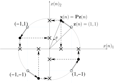
Figure 2: Displaying the rotation at the transmitter 2 and at the receiver (without noise) 2 for $B=2$. The empty (filled) circles represent $\Omega_{z}$ ($\Omega_{x}$). The components of $\mathbf{t}(n)$ are obtained by scaling the components $\mathbf{x}(n)$ by their respective fading gain (here $\alpha_{2}<\alpha_{1}$), as expressed by the component-wise multiplication $\boldsymbol{\alpha}\cdot\mathbf{x}(n)$. The crosses on the coordinate axes are the transmitted 2 and received 2 vector components, respectively.

Considering $\mathbf{t}(n)$, an equivalent channel model can be formulated:

$$\mathbf{y}(n)=\mathbf{t}(n)+\mathbf{w}(n),~{}~{}n=1,\ldots,\frac{N}{B},$$ (9)

which yields more insight and will be useful in the proofs of propositions of this paper. This system model represents a Gaussian vector channel with input $\mathbf{t}(n)$. This means that for a particular fading point, the block fading channel can be interpreted as a virtual Gaussian channel, with a discrete input alphabet $\Omega_{t}$.

III Analysis of Outage Probability in the fading space

For the remainder of the paper, we will drop the index $n$ in the vectors $\mathbf{z}(n)$, $\mathbf{x}(n)$, $\mathbf{t}(n)$, $\mathbf{y}(n)$ and $\mathbf{w}(n)$, as the time index is not important when considering mutual information. We write random variables using upper case letters corresponding to the lower case letters used for their realizations. The mutual information $I\left(\boldsymbol{\alpha},\gamma,P\right)$ at a certain fading point $\boldsymbol{\alpha}$ between the transmitted B-dimensional symbol $\mathbf{x}$ (uniformly distributed over $\Omega_{x}$) and the corresponding received vector $\mathbf{y}$ is given by

$$I\left(\boldsymbol{\alpha},\gamma,P\right)=\frac{1}{B}I(\mathbf{X};\mathbf{Y}|\boldsymbol{\alpha},\gamma),$$ (10)

where the scaling factor $\frac{1}{B}$ is added because the $B$ blocks in the channel timeshare a time-interval [5, Section 9.4], [32, Section 5.4.4]. The mutual information $I(\mathbf{X};\mathbf{Y}|\boldsymbol{\alpha},\gamma)$ is [12], [10]

$$I(\mathbf{X};\mathbf{Y}|\boldsymbol{\alpha},\gamma)=m-2^{-m}\sum_{\mathbf{x}\in\Omega_{x}}\mathbb{E}_{\mathbf{y}|\mathbf{x}}\left[\textrm{log}_{2}\left(\sum_{\mathbf{x}^{{}^{\prime}}\in\Omega_{x}}\exp\left[\frac{d^{2}(\mathbf{y},\boldsymbol{\alpha}\cdot\mathbf{x})-d^{2}(\mathbf{y},\boldsymbol{\alpha}\cdot\mathbf{x}^{\prime})}{2\sigma^{2}}\right]\right)\right],$$ (11)

where $d^{2}(\mathbf{v},\mathbf{u})=\sum_{b=1}^{B}\left|v_{b}-u_{b}\right|^{2}$. However, more insight can be gained when considering $\mathbf{t}$. From Eq. (9), it is clear that for a certain fading point, the mutual information of this virtual channel, with input $\Omega_{t}$, is the same as the mutual information of the actual channel, with input $\Omega_{x}$,

$$I\left(\boldsymbol{\alpha},\gamma,P\right)=\frac{1}{B}I(\mathbf{T};\mathbf{Y}|\boldsymbol{\alpha},\gamma).$$ (12)

Hence, the fading point $\boldsymbol{\alpha}$ maximizing (minimizing) the mutual information $I(\mathbf{X};\mathbf{Y}|\boldsymbol{\alpha},\gamma)$ corresponds to the fading point that distorts constellation $\Omega_{t}$ in the best (worst) way at the input of a Gaussian vector channel. This interpretation allows to exploit the many results from literature on the mutual information of Gaussian channels. Therefore, Eq. (12) will be useful in the following.

The outage probability is the probability that the instantaneous mutual information is less than the transmitted information bitrate $R$ [32, section 5.4],

$$P_{\textrm{out}}(\gamma,P,R)=\textrm{Pr}\big{(}I\left(\boldsymbol{\alpha},\gamma,P\right)<R\big{)}.$$ (13)

Our main goal is to find the precoding matrix $P$ that minimizes the outage probability $P_{\textrm{out}}(\gamma,P,R)$,

$$P_{\textrm{opt}}=\underset{P}{\operatorname{argmin}}~{}P_{\textrm{out}}(\gamma,P,R).$$

A closed form expression for $I\left(\boldsymbol{\alpha},\gamma,P\right)$ does not exist and Eq. (11) is difficult to analyze because of the presence of the mathematical expectation. Therefore, in the following two sections, we will develop simple bounds on the outage probability and will approximate $P_{\textrm{opt}}$ by the optimal precoding matrix that minimizes the bounds on the outage probability.

But first we will introduce a framework in this section that allows to gain insight on the meaning of the outage probability. The considered framework is the fading space [4], which is the B-dimensional Euclidean space, ${\mathbb{R}^{+}}^{B}$, of the real-valued positive fading gains. The outage probability equals the probability that the fading point $\boldsymbol{\alpha}$ belongs to a region $V_{\textrm{o}}$, which is such that $I\left(\boldsymbol{\alpha},\gamma,\theta\right)<R$ for all $\boldsymbol{\alpha}$ in $V_{\textrm{o}}$ (Fig. 3(a)):

$$P_{\textrm{out}}(\gamma,P,R)=\int_{\boldsymbol{\alpha}\in V_{\textrm{o}}}p(\boldsymbol{\alpha})\mathrm{d}\boldsymbol{\alpha},$$ (14)

where $p(\boldsymbol{\alpha})$ is the joint pdf of the fading gains $\alpha_{1},\ldots,\alpha_{B}$. We say that the region $V_{\textrm{o}}$ is limited by an outage boundary $B_{\textrm{o}}(\gamma,P,R)$ (see Fig. 3(a) for $B=2$), defined by

$$I\left(\boldsymbol{\alpha},\gamma,P\right)=R,~{}~{}\forall~{}\boldsymbol{\alpha}\in B_{\textrm{o}}(\gamma,P,R).$$

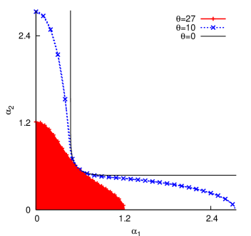
(a) Examples of an outage boundary when $\Omega_{z}=$ $4$-$\mathcal{R}^{2}$ and the rotation angle is $\theta=0,10,27$ degrees. The region $V_{\textrm{o}}$ is coloured red for $\theta=27$ degrees.

(b) The points $\{\alpha_{b,\textrm{o}}$, $b=1,\ldots,B\}$ and $\alpha_{\textrm{e}}$ are shown for $B=2$.

Figure 3: The outage boundary limits the outage region $V_{\textrm{o}}$ in the fading space which corresponds to an information theoretic outage event. In the Figure, the information rate is $R=0.9$ bpcu and the average SNR is fixed to $\gamma=8$ dB.

In general, we can consider a certain boundary in the fading space limiting a certain region $V$. This boundary is denoted by $B(V)$. The outage boundary $B_{\textrm{o}}(\gamma,P,R)$ corresponds to the region $V_{\textrm{o}}$, as defined in (14), so that the outage boundary is $B_{\textrm{o}}(\gamma,P,R)=B(V_{\textrm{o}})$.

Definition 1

We define $\alpha_{b,\textrm{o}}$ by the magnitude of the intersection between the outage boundary and the axis $\alpha_{b}$. More precisely, $I\left(\boldsymbol{\alpha}\arrowvert_{\alpha_{i}=0,i\neq b,\alpha_{b}=\alpha_{b,\textrm{o}}},\gamma,P\right)=R$. By convention, $\alpha_{b,\textrm{o}}=+\infty$ if the axis $\alpha_{b}$ is an asymptote for the outage boundary. It is possible that $\alpha_{b,\textrm{o}}$ does not exist.

Definition 2

We define $\alpha_{\textrm{e}}$ as the value of the components of the intersection between the outage boundary and the line $\alpha_{1}=\ldots=\alpha_{B}$ (also known as the ergodic line). More precisely, $I\left(\boldsymbol{\alpha}\arrowvert_{\alpha_{i}=\alpha_{\textrm{e}},i\in[1,\ldots,B]},\gamma,P\right)=R$.

The defined points are illustrated in Fig. 3(b) for $B=2$. In the remainder of the paper, we denote the points $\boldsymbol{\alpha}\arrowvert_{\alpha_{i}=0,i\neq b,\alpha_{b}=\alpha_{b,\textrm{o}}}$ by $\boldsymbol{\alpha}_{b,\textrm{o}}$ and $\boldsymbol{\alpha}\arrowvert_{\alpha_{i}=\alpha_{\textrm{e}},i\in[1,\ldots,B]}$ by $\boldsymbol{\alpha}_{\textrm{e}}$.

Proposition 1

On a BF channel with $B=2$, with a discrete input alphabet and with linear precoding, the magnitudes $\{\alpha_{b,\textrm{o}},~{}b=1,2\}$ are equal if the constellation is invariant under a rotation of 90 degrees and the precoding matrix is orthogonal.
On a BF channel with $B>2$, with a discrete input alphabet and with linear precoding, the magnitudes $\{\alpha_{b,\textrm{o}},~{}b=1,\ldots,B\}$ are equal if the constellation is invariant under a cyclic shift of the components of the points of the constellation and the precoding matrix is an orthogonal circulant matrix.

Proof:

See Appendix -A. ∎

Notice that the condition of Prop. 1 is a sufficient condition and not a necessary condition. In the remainder of this paper, it is assumed that the constellation used at the transmitter fulfils Prop. 1. The magnitudes $\{\alpha_{b,\textrm{o}},b=1,\ldots,B\}$ will then simply be denoted by $\alpha_{\textrm{o}}$. This also means that the projection of $\Omega_{x}$ on either coordinate axes yields the same set of points, which we denote by $\mathcal{S}_{\textrm{p}}$, where $p$ stands for projection.

Note that a multidimensional constellation that fulfils Prop. 1 (i.e., its projection on each coordinate axis yields the same set of points, see Appendix -A) has an interesting property. For these constellations, the function $I\left(X_{b};Y_{b}|\alpha_{b}=\alpha,\gamma\right)$, which is the mutual information of a point-to-point channel with fading coefficient $\alpha_{b}=\alpha$, average SNR $\gamma$ and with discrete input $X_{b}$, does not depend on $b$. As a consequence, we will represent this mutual information by $I_{\mathcal{S}_{\textrm{p}}}\left(\alpha^{2}\gamma,P\right)$.

Definition 3

Boundary $B_{1}=B(V_{1})$ is said to outer bound outage boundary $B_{2}=B(V_{2})$ if $V_{2}\subseteq V_{1}$. The opposite holds for inner bounding.

The outage boundary in the fading space has a simple but interesting property: if an outage boundary outer bounds (inner bounds) another outage boundary, than its corresponding outage probability is larger (smaller) (see Eq. (14)). For example, consider the input alphabet $\mathbf{Z}\sim\mathcal{N}(\mathbf{0},I)$, which we denote as an i.i.d. Gaussian input alphabet, where $\mathbf{0}$ is a column vector of zeros and $I$ is the identity matrix. We denote the outage boundary (outage region) corresponding to i.i.d. Gaussian inputs and discrete input alphabets, by $B_{\textrm{o}}\textrm{(Gauss)}$ ($V_{\textrm{o}}\textrm{(Gauss)}$) and $B_{\textrm{o}}\textrm{(discrete)}$ ($V_{\textrm{o}}\textrm{(discrete)}$), respectively. The boundary $B_{\textrm{o}}\textrm{(Gauss)}$ inner bounds $B_{\textrm{o}}\textrm{(discrete)}$ [5]. Therefore, the outage probability corresponding to i.i.d. Gaussian inputs is a lower bound on the outage probability corresponding to a discrete input alphabet. Consequently, by minimizing the outage probability corresponding to a discrete input alphabet, $B_{\textrm{o}}\textrm{(discrete)}$ can at most approach $B_{\textrm{o}}\textrm{(Gauss)}$ (see Fig. 4).

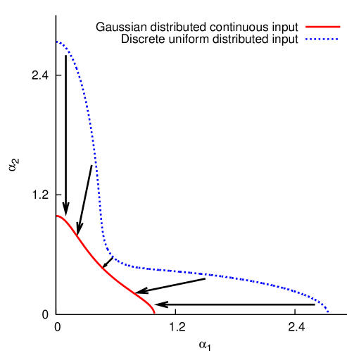
Figure 4: The outage boundary $B_{\textrm{o}}\textrm{(discrete)}$ is inner bounded by $B_{\textrm{o}}\textrm{(Gauss)}$. Optimizing the precoding matrix can at most make $B_{\textrm{o}}\textrm{(discrete)}$ approach $B_{\textrm{o}}\textrm{(Gauss)}$ as illustrated by the arrows.

In the following two sections, we will determine boundaries with simple shapes outer (inner) bounding $B_{\textrm{o}}\textrm{(discrete)}$, which are then much easier to optimize. For the outer boundary, this can be done by determining a surface in the fading space, $U(\boldsymbol{\alpha})=0$, satisfying

$$I\left(\boldsymbol{\alpha},\gamma,P\right)\geq R,~{}\textrm{for all }\boldsymbol{\alpha}\textrm{ satisfying }U(\boldsymbol{\alpha})=0.$$ (15)

For the inner boundary, the greater than or equal sign is replaced by a smaller than or equal sign. For example, for $B=2$, we will prove that a circular arc touching $B_{\textrm{o}}\textrm{(discrete)}$ at $\alpha_{1}=\alpha_{\textrm{o}}$ (on the horizontal axis) and $\alpha_{2}=\alpha_{\textrm{o}}$ (on the vertical axis) satisfies Eq. (15).

IV Bounds on the outage probability without linear precoding

As a first step, we will establish upper and lower bounds on the outage probability of a communication system without linear precoding. This will set the stage for the bounds with linear precoding in Sec. V.

We will prove that the outage region is outer bounded by a $B$-hypersphere touching the outage boundary on the axes of the fading space, hence with radius $\alpha_{\textrm{o}}$. A $B$-hypersphere $U(\boldsymbol{\alpha})=0$ is a generalization of a sphere to $B$ dimensions,

$$U(\boldsymbol{\alpha})=\sum_{b=1}^{B}\alpha_{b}^{2}-\alpha_{\textrm{o}}^{2}.$$

Note that this is only possible for constellations fulfilling the conditions of Prop. 1. For other constellations, the outer bounding $B$-hypersphere will have a radius of $\max_{b\in[1,\ldots,B]}\alpha_{b,\textrm{o}}$ and will therefore be less tight.

Next, we will prove that the outage region is inner bounded by a $B$-hypersphere touching the outage boundary at $\boldsymbol{\alpha}_{\textrm{e}}$.

Lemma 1

On a BF channel with a discrete multidimensional input alphabet $\mathbf{X}$, the mutual information $I\left(\boldsymbol{\alpha},\gamma,P\right)$ is upper bounded as follows

$$I\left(\boldsymbol{\alpha},\gamma,P\right)\leq\frac{1}{B}\sum_{b=1}^{B}I_{\mathcal{S}_{\textrm{p}}}\left(\alpha_{b}^{2}\gamma,P\right).$$ (16)

Proof:

See Appendix -B. ∎

A special case is the case without precoding ($P=I$) so that $\Omega_{x}=\Omega_{z}$. If in that case $\Omega_{z}$ is the Cartesian product of $\Omega_{z_{1}}$, …, $\Omega_{z_{B}}$ , $\Omega_{z}=(\mathcal{S}_{\textrm{p}})^{B}$, then all variables $X_{b}=Z_{b}$ are independent for all $b$, so that equality holds in Eq. (16). E.g., $\Omega_{z}=$ $4$-$\mathcal{R}^{2}$, as shown in Fig. 2, is the Cartesian product of two BPSK constellations, denoted as BPSK$\times$BPSK.

For an i.i.d. Gaussian input alphabet, the instantaneous mutual information with linear precoding is the same as the instantaneous mutual information without linear precoding, because $P\mathbf{z}=\mathbf{x}\sim\mathcal{N}(\mathbf{0},I)$ when $P$ is orthogonal, so that precoding does not change the distribution of the input vector. Therefore, the instantaneous mutual information for an i.i.d. Gaussian input alphabet is

$$I\left(\boldsymbol{\alpha},\gamma,P\right)=I\left(\boldsymbol{\alpha},\gamma,P=I\right)=\frac{1}{B}\sum_{b=1}^{B}0.5~{}\textrm{log}_{2}(1+2\gamma\alpha_{b}^{2}).$$ (17)

Proposition 2

The outage region $V_{\textrm{o}}\textrm{(Gauss)}$ of a BF channel with an i.i.d. Gaussian input alphabet is outer bounded by the $B$-hypersphere $\alpha_{1}^{2}+\alpha_{2}^{2}+\ldots+\alpha_{B}^{2}=\frac{4^{BR}-1}{2\gamma}$ and inner bounded by the $B$-hypersphere $\alpha_{1}^{2}+\alpha_{2}^{2}+\ldots+\alpha_{B}^{2}=\frac{4^{R}-1}{2\gamma}$.

Proof:

In Appendix -C, it is proved that for $\boldsymbol{\alpha}$ on a hypersurface:

• $I\left(\boldsymbol{\alpha},\gamma\right)\arrowvert_{\alpha_{1}=\ldots=\alpha_{B}}\geq I\left(\boldsymbol{\alpha},\gamma\right)$

• $I\left(\boldsymbol{\alpha},\gamma\right)\arrowvert_{\alpha_{b}=\alpha_{\textrm{o}}}\leq I\left(\boldsymbol{\alpha},\gamma\right)$,

because the mutual information is a sum of concave functions of the instantaneous SNRs $\gamma\alpha_{b}^{2}$ (Eq. (17)). Calculating $\alpha_{\textrm{o}}$ and $\alpha_{\textrm{e}}$, according to Definitions 1 & 2, yields the radii of both $B$-hyperspheres. ∎

The inner boundary touches the outage boundary in the point $\boldsymbol{\alpha}_{\textrm{e}}$, so that it does not depend on $B$ (the entire codeword is affected by the same fading gain $\alpha_{\textrm{e}}$). The outer boundary touches the outage boundary in the points $\boldsymbol{\alpha}_{b,\textrm{o}}$, $\forall~{}b$; its dependence on $B$ follows from the fact that $B-1$ is equal to the number of erased channels.

Proposition 3

On a BF channel with a discrete input alphabet $\Omega_{z}$ that is a Cartesian product of one-dimensional constellations, the outage region $V_{\textrm{o}}\textrm{(discrete)}$ is outer bounded by the $B$-hypersphere $\alpha_{1}^{2}+\alpha_{2}^{2}+\ldots+\alpha_{B}^{2}=\alpha_{\textrm{o}}^{2}$ touching it at the axes of the fading space at $\boldsymbol{\alpha}_{b,\textrm{o}}$, $\forall~{}b$. Also, $V_{\textrm{o}}\textrm{(discrete)}$ is inner bounded by the $B$-hypersphere $\alpha_{1}^{2}+\alpha_{2}^{2}+\ldots+\alpha_{B}^{2}=B\alpha_{\textrm{e}}^{2}$ touching it at $\boldsymbol{\alpha}_{\textrm{e}}$.

Proof:

Lemma 1 proved that the mutual information is upper bounded by $\frac{1}{B}\sum_{b=1}^{B}I_{\mathcal{S}_{\textrm{p}}}\left(\alpha_{b}^{2}\gamma,P\right)$, where this upper bound coincides with the exact expression in the case that $\Omega_{z}$ is a Cartesian product. Using the relation between the mutual information $I(\textrm{SNR})=I_{\mathcal{S}_{\textrm{p}}}\left(\alpha_{b}^{2}\gamma,P\right)$ and the minimum mean-square error (MMSE) in estimating the input symbol, $X_{b}\in\mathcal{S}_{\textrm{p}}$, given the output symbol $Y_{b}$ [15],

$$\frac{\textrm{d}}{\textrm{d SNR}}I(\textrm{SNR})=\frac{1}{2}\textrm{MMSE}(\textrm{SNR}),$$ (18)

it is easily proved that $I_{\mathcal{S}_{\textrm{p}}}\left(\alpha_{b}^{2}\gamma,P\right)$ is a concave function (the second derivative is negative) of the instantaneous SNR $\gamma\alpha_{b}^{2}$, because the MMSE is a decreasing function of the SNR. Therefore, the proof is the same as for Prop. 2. ∎

Notice that the techniques of the proofs of Props. 2 and 3 cannot be used for discrete input alphabets $\Omega_{z}$ that are not a Cartesian product of one-dimensional constellations, because in that case the upper bound $\frac{1}{B}\sum_{b=1}^{B}I_{\mathcal{S}_{\textrm{p}}}\left(\alpha_{b}^{2}\gamma,P\right)$ does not coincide with the exact expression of the mutual information. However, this case is merely a particular case ($P=I$) of a precoded discrete input alphabet, which is covered in the next section.

V Bounds on the outage probability with linear precoding

Propositions 2 and 3 mainly state that the outage region for a channel with an i.i.d. Gaussian input alphabet or a discrete input alphabet without precoding is outer (inner) bounded by a $B$-hypersphere touching it at $\boldsymbol{\alpha}_{b,\textrm{o}},~{}\forall~{}b$ ($\boldsymbol{\alpha}_{\textrm{e}}$). We conjecture that this property still holds for a communication system with a discrete alphabet with linear precoding at the input of the channel. First, we will give new detailed proofs for low and high instantaneous SNR of this property. Then, a more intuitive explanation will be given to provide more insight.

Proposition 4

On a BF channel at low instantaneous SNR, with a discrete input alphabet and with linear precoding, the outage region $V_{\textrm{o}}\textrm{(discrete)}$ is outer (inner) bounded by the $B$-hypersphere $\alpha_{1}^{2}+\alpha_{2}^{2}+\ldots+\alpha_{B}^{2}=\alpha_{\textrm{o}}^{2}$ ($\alpha_{1}^{2}+\alpha_{2}^{2}+\ldots+\alpha_{B}^{2}=B\alpha_{e}^{2}$).

Proof:

See Appendix -D. ∎

Proposition 5

On a BF channel at high instantaneous SNR, with a discrete input alphabet and with linear precoding, the outage region $V_{\textrm{o}}\textrm{(discrete)}$ is outer (inner) bounded by the $B$-hypersphere $\alpha_{1}^{2}+\alpha_{2}^{2}+\ldots+\alpha_{B}^{2}=\alpha_{\textrm{o}}^{2}$ ($\alpha_{1}^{2}+\alpha_{2}^{2}+\ldots+\alpha_{B}^{2}=B\alpha_{e}^{2}$).

Proof:

See Appendix -E. ∎

The outer and inner bound touch the outage boundary at the axes of the fading space and on the ergodic line, respectively. The outer (inner) region corresponds to an upper (lower) bound on the outage probability. Minimizing this upper (lower) bound is simply achieved by minimizing $\alpha_{\textrm{o}}$ ($\alpha_{e}$).

To get more insight, we give an illustration of Props. 4 and 5. We consider the $4$-$\mathcal{R}^{2}$ constellation $\Omega_{x}$ from Fig. 2, with $\theta=\pi/6$. Further, we take $\alpha_{1}=\alpha_{\textrm{o}}\cos(\lambda)$ and $\alpha_{2}=\alpha_{\textrm{o}}\sin(\lambda)$, i.e., $|\boldsymbol{\alpha}|=\alpha_{\textrm{o}}$, so that $\boldsymbol{\alpha}$ is on the outer boundary of the outage boundary. Fig. 5 shows the corresponding mutual information $I(\boldsymbol{\alpha},\gamma,\theta)$ as a function of $\gamma$ for various values of $\lambda$. We observe that the mutual information increases when $\lambda$ increases from $0$ to $\pi/4$. The projections of the constellation $\Omega_{t}$ on the horizontal and vertical coordinate axes have variances $\alpha_{1}^{2}=\alpha_{\textrm{o}}^{2}\cos^{2}(\lambda)$ and $\alpha_{2}^{2}=\alpha_{\textrm{o}}^{2}\sin^{2}(\lambda)$ respectively, whereas the total variance of $\Omega_{t}$ equals $\alpha_{\textrm{o}}^{2}$, irrespective of $\lambda$. When $\lambda=\pi/4$, $\Omega_{t}$ is equivalent to a common QPSK constellation: the variances of both projections equal $\frac{\alpha_{\textrm{o}}^{2}}{2}$, and the corresponding mutual information is maximum. When $\lambda$ decreases from $\pi/4$ to $0$, the difference between the two variances increases, $\Omega_{t}$ becomes an increasingly more distorted QPSK constellation, and the mutual information decreases. At $\lambda=0$ we get $\alpha_{1}=\alpha_{\textrm{o}}$ and $\alpha_{2}=0$; $\Omega_{t}$ (which is now a scaling of $\mathcal{S}_{\textrm{p}}$) reduces to a 4-PAM constellation and the corresponding mutual information is minimum. This illustrates the general principle that performance is optimized when the transmit power is equally split over the available identical channels and the performance is worst when the transmit power is completely used for only one channel, which is exactly what is claimed in Props. 4 and 5 for high and low instantaneous SNR. More specifically, for $\boldsymbol{\alpha}$ on the hypersurface of a hypersphere, it is proved in Props. 4 and 5 that the mutual information is the smallest at $\boldsymbol{\alpha}_{b,\textrm{o}}$, and the largest at $\boldsymbol{\alpha}_{e}$.

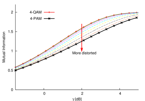
Figure 5: The mutual information is monotonically non-increasing as the constellation becomes more distorted. The upper and lower curve correspond to $\lambda=\pi/4$ and $\lambda=0$ respectively.

Prop. 6 states the condition under which the precoded constellations achieve full diversity for a rate $R$. This is proved in [12], but based on Prop. 5, a new simple proof can be given.

Proposition 6

For any coding rate $0<R_{c}<1$, the outage probability of a Rayleigh distributed block fading channel with $B$ blocks, with a discrete input alphabet and linear precoding exhibits full diversity, i.e., $P_{\textrm{out}}(\gamma,P,R)\propto 1/\gamma^{B}$ at large $\gamma$, if $2^{BR}$ does not exceed the number of points contained in the projection of the precoded input constellation $\Omega_{x}$ on a coordinate axis.

Proof:

See Appendix -F. ∎

It should be noted that the proof of Prop. 6 assumes the existence of $I_{\mathcal{S}_{\textrm{p}}}^{-1}(BR,P)$; hence, the number of points in $\mathcal{S}_{\textrm{p}}$ must not be less than $2^{BR}$. We consider the $4$-$\mathcal{R}^{2}$ constellation from Fig. 2 to illustrate the constraint on the existence of $I_{\mathcal{S}_{\textrm{p}}}^{-1}(BR,P)$. For $4$-$\mathcal{R}^{2}$ from Fig. 2, $\mathcal{S}_{\textrm{p}}$ contains only $2$ points when the rotation angle $\theta$ is a multiple of $\pi/2$, $3$ points when the rotation angle $\theta$ is a multiple of $\pi/4$ but not of $\pi/2$, and $4$ points otherwise, yielding $R=0.5$, $R=3/4$ and $R=1$, respectively, as maximal rates corresponding to full diversity.

VI Optimization of the outage probability of precoded constellations

In the previous section, we established that, for high and low instantaneous SNR, the outage region of block fading channels with precoded constellations is outer bounded by a $B$-hypersphere with center in the origin and touching the outage boundary on the axes of the fading space. This hypersphere corresponds to an upper bound on the outage probability of the channel (see the paragraph after Def. 3). Instead of minimizing the actual outage probability, it is easier to minimize the upper bound on the outage probability. This optimization will allow the actual outage probability to closely approach a lower bound on the outage probability, i.e., the outage probability corresponding to an i.i.d. Gaussian input alphabet, as we will see in the numerical results.

The $B$-hypersphere is completely determined by one variable, its radius $\alpha_{\textrm{o}}$. We denote the $B$-hypersphere outer bounding the outage region by $V_{\textrm{up}}(\alpha_{\textrm{o}})$ and the corresponding upper bound on the outage probability by $P_{\textrm{up}}(\alpha_{\textrm{o}})$:

$$P_{\textrm{up}}(\alpha_{\textrm{o}})=\int_{\boldsymbol{\alpha}\in V_{\textrm{up}}(\alpha_{\textrm{o}})}p(\boldsymbol{\alpha)}\mathrm{d}\boldsymbol{\alpha}.$$ (19)

From Eq. (19), it is clear that the region $V_{\textrm{up}}(\alpha_{\textrm{o}})$ has to be made as small as possible to minimize $P_{\textrm{up}}(\alpha_{\textrm{o}})$. Therefore, the optimization target is to minimize the radius $\alpha_{\textrm{o}}$.

Because $I_{\mathcal{S}_{\textrm{p}}}(\alpha_{\textrm{o}}^{2}\gamma,P)=BR$, the minimization of $\alpha_{\textrm{o}}$ (and, therefore, the minimization of the upper bound on the outage probability) is achieved by selecting the constellation $\mathcal{S}_{\textrm{p}}$ requiring the least energy to achieve a rate $BR$ on a Gaussian channel. This involves a proper selection of both the constellation $\Omega_{z}$ and the precoding matrix $P$. Note that this optimization is much simpler than the direct minimization of the outage probability as given by Eqs. (13) and (10), because the outage probability is hard to evaluate, especially when the number of fading gains and constellation points is large. Furthermore, no insight is gained by the latter approach, so that it would not be clear which constellation $\Omega_{z}$ should be taken.

(a) The transmitted symbols are the components $x_{b}$ of the constellation $\Omega_{x}$.

(b) The received symbols $t_{b}$ are the faded components $\alpha_{b}x_{b}$. Collecting the different components $t_{b}$, the faded constellation $\Omega_{t}$ is constructed, which is expressed by $\Omega_{t}=\boldsymbol{\alpha}\cdot\Omega_{x}$.

Figure 6: The transmitted ($\Omega_{x}$) and faded constellation ($\Omega_{t}$) are shown for the case of the transmission of real-valued symbols, $B=2$ and $\Omega_{z}=8$-$\mathcal{R}^{2}$. For $\Omega_{t}=\boldsymbol{\alpha}\cdot\Omega_{x}$, the fading point $(\alpha_{1,\textrm{o}},0)$, the intersection between the outage boundary and the axis $\alpha_{2}=0$, is used.

Also, the outage region of block fading channels with precoded constellations is inner bounded by a $B$-hypersphere with center in the origin and touching the outage boundary in the point $\boldsymbol{\alpha}_{\textrm{e}}$. Hence, $\alpha_{\textrm{e}}$ determines the radius of this $B$-hypersphere, $\sqrt{B}\alpha_{\textrm{e}}$. In this point, the faded constellation $\Omega_{t}$ is balanced, as in Fig. 6(a). We will denote this balanced constellation $\Omega_{t}=\boldsymbol{\alpha}_{\textrm{e}}\cdot\Omega_{x}$ by $\mathcal{S}_{\textrm{e}}$. Hence, the hypersphere corresponds to a lower bound on the outage probability which is minimized by optimizing the mutual information of $\mathcal{S}_{\textrm{e}}$.

In this section, we will show that the radius of the outer region, $\alpha_{\textrm{o}}$, and the radius of the inner region, $\sqrt{B}\alpha_{\textrm{e}}$, can be minimized by combining a simple optimization of the precoding matrix $P$ with a constellation expansion.

VI-A Optimization of the precoding matrix

Precoding corresponds to performing a unitary transformation of the input vector $\mathbf{x}$. As a unitary transformation preserves distance, it follows from Eq. (11) that the value $\alpha_{\textrm{e}}$ is insensitive to orthogonal transformations. Hence, the selection of the precoding matrix $P$ affects only the radius of the outer region $\alpha_{\textrm{o}}$. Let us denote by $\mathcal{O}$ the set of parameters from $P$ over which we will minimize $\alpha_{\textrm{o}}$. For $B=2$ and $B=3$, the only degree of freedom is the rotation angle (see (4) and (8)). For $B>3$, more degrees of freedom can be exploited to minimize $\alpha_{\textrm{o}}$. For the numerical results, we restrict ourselves to $B\leq 3$.

The mutual information of $\mathcal{S}_{\textrm{p}}$ can be rewritten as $I_{\mathcal{S}_{\textrm{p}}}(\alpha_{\textrm{o}}^{2}\gamma,\mathcal{O})$, which yields $\alpha_{\textrm{o}}^{2}=\frac{I_{\mathcal{S}_{\textrm{p}}}^{-1}(BR,\mathcal{O})}{\gamma}$. Changing the value of $\mathcal{O}$ (e.g. the rotation angle $\theta$ for $B=2$) will change the distances between the points in $\mathcal{S}_{\textrm{p}}$ and so change its mutual information. For a fixed spectral efficiency $R$ and fixed average SNR $\gamma$, minimizing the radius yields the optimization criterion

$$\mathcal{O}_{\textrm{opt}}=\underset{\mathcal{O}}{\operatorname{argmin}}~{}I_{\mathcal{S}_{\textrm{p}}}^{-1}(BR,\mathcal{O}).$$

The optimization is performed by means of a simulation, due to the lack of closed form expressions of the mutual information. Because the constellation is one-dimensional, the computational effort is minimal. We apply this optimization for different scenarios in Sec. VII.

VI-B Constellation expansion

As the number of information bits per channel use is $R=mR_{c}/B$, there are different combinations of $m$ and $R_{c}$ yielding the same $R$. Taking into account that $R_{c}\leq 1$, the minimum value of $m$ equals $\lceil BR\rceil$, with a corresponding coding rate $R_{c}=\frac{BR}{\lceil BR\rceil}$.

The number of points in the constellation is $|\Omega_{t}|$. Increasing the constellation size of $\Omega_{z}$ will render a constellation $\Omega_{t}$ with more points, both for $\mathcal{S}_{\textrm{e}}$ and $\mathcal{S}_{\textrm{p}}$. This higher order constellation may need less energy to achieve the same rate, both for the balanced case (optimization of $\alpha_{e}$) as the distorted case (optimization of $\alpha_{\textrm{o}}$). However, the decoding complexity increases as well as the complexity of optimization, so that there is a trade-off between performance and complexity. The higher the constellation size, the smaller the horizontal SNR-gap between the outage probabilities corresponding to a precoded discrete input alphabet and i.i.d. Gaussian input alphabet. However, the improvement in performance becomes smaller and smaller, as illustrated in Sec. VII.

VII Numerical results

VII-A Numerical results for $B=2$

When $B=2$, $\mathcal{O}=\theta$, and the optimization criterion for the upper bound on the outage probability is to find $\theta$ so that $I_{\mathcal{S}_{\textrm{p}}}^{-1}(BR,\theta)$ is minimized. Next, a constellation expansion is performed to further minimize the upper bound as well as the lower bound on the outage probability.

VII-A1 Real constellations

Assume that a transmission rate $R=0.9$ bpcu is aimed. First, we consider the optimization of the rotation angle $\theta$, see Fig. 7. On the left $y$-axis, we show the instantaneous SNR per symbol, $\gamma_{\textrm{s}}=\alpha_{\textrm{o}}^{2}\gamma$, so that $I_{\mathcal{S}_{\textrm{p}}}(\gamma_{\textrm{s}},\theta)=BR$. The minimum SNR per symbol $\gamma_{\textrm{s}}$ that is needed to transmit $R=0.9$ bpcu for $\gamma=8$ dB is achieved by an i.i.d. Gaussian input alphabet:

$$\gamma_{\textrm{s}}=\frac{2^{4R}-1}{2}.$$

This fundamental minimum can be approached when using a precoded discrete input $\Omega_{z}=4$-$\mathcal{R}^{2}$ ($R_{c}=0.9$) with rotation angle $\theta=27$ degrees. Now, we apply a constellation expansion to further reduce $\alpha_{\textrm{o}}$ (see Fig. 7) and $\alpha_{\textrm{e}}$ (see Fig. 8). For example, $\gamma_{\textrm{s}}$ for the rotated constellation $\Omega_{z}=8$-$\mathcal{R}^{2}$ ($R_{c}=0.6$) approaches the theoretical minimum very closely for rotation angles within $[0\ldots 9]$ degrees. An expansion to $\Omega_{z}=16$-$\mathcal{R}^{2}$ ($R_{c}=0.45$ and $\theta_{\textrm{opt}}\in[35,45]$ degrees) only slightly improves the performance. The optimization of $\gamma_{\textrm{s}}$ decreases the volume of the region $V_{\textrm{o}}$, which is illustrated in Fig. 3(a) for $\Omega_{z}=4$-$\mathcal{R}^{2}$. Fig. 8 illustrates that constellation expansion is sufficient to reduce the value $\alpha_{\textrm{e}}$, which is very close to the theoretical minimum. Therefore, the constellation is not further shaped to minimize the lower bound of the outage probability.

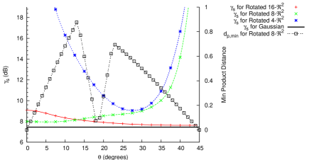
Figure 7: The optimization of the radius of the outer region is shown for $\Omega_{z}=4$-$\mathcal{R}^{2}$, $R=0.9$ bpcu and $\gamma=8$ dB. The y-axis at the left denotes the instantaneous SNR per symbol, $\gamma_{\textrm{s}}=\alpha_{\textrm{o}}^{2}\gamma$, and the right y-axis denotes the minimum product distance. The thick black line without markers represents the fundamental minimum SNR per symbol, $\gamma_{\textrm{s}}$, that is needed to transmit $R=0.9$ bpcu for $\gamma=8$ dB, i.e., when using an i.i.d. Gaussian input alphabet. The effect of constellation expansion on the radius $\alpha_{\textrm{o}}$ is shown by optimization of $\Omega_{z}=8$-$\mathcal{R}^{2}$ and $\Omega_{z}=16$-$\mathcal{R}^{2}$. The profile of the minimum product distance, $d_{p,\textrm{min}}$, is shown for $\Omega_{z}=8$-$\mathcal{R}^{2}$.

The information theoretic approach used in this paper does not lead to the same optimized rotations as in the case of algebraic constructions of uncoded constellations. In [3] and [1], multidimensional rotations have been optimized for uncoded infinite constellations transmitted on ergodic fading channels. As a simple illustration, we show in Fig. 7 the minimum product distance $d_{p,\textrm{min}}$ [32] of the uncoded $8$-$\mathcal{R}^{2}$ versus the rotation angle. The optimum and the profile of $d_{p,\textrm{min}}$ and those of $\gamma_{\textrm{s}}$ do not match. The minimum product distance approach is not suitable for coded schemes. For example, the minimum product distance is zero for $\theta=0$ degrees, while this rotation angle is optimal in terms of outage probability.

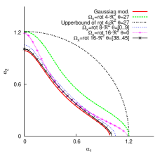
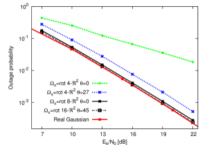
Figure 8: The outage boundaries (left) and outage probabilities (right) of $\Omega_{z}=4$-$\mathcal{R}^{2}$, $\Omega_{z}=8$-$\mathcal{R}^{2}$ and $\Omega_{z}=16$-$\mathcal{R}^{2}$ with and without optimized rotation angle are shown. The spectral efficiency is $R=0.9$ bpcu and $\gamma=8$ dB (left).

The outage probabilities of the considered multidimensional constellations are shown in Fig. 8. This confirms that constellation expansion together with the optimization of the precoding parameter is sufficient to approach the outage probability with an i.i.d. Gaussian input alphabet very closely. It also shows that the constellation $\Omega_{x}=8$-$\mathcal{R}^{2}$ with $\theta\in$ $[0\ldots 9]$ degrees represents the best trade-off between performance and complexity.

VII-A2 Extension to complex constellations

All the proofs in this paper are valid for complex constellations. This means that also for complex constellations, the outage region is outer bounded by a $B$-hypersphere, determined by one variable, its radius. We restrict our attention to real-valued precoding matrices. Consider Eq. (2), where $\mathbf{z}$ is now a complex vector and $P$ is real-valued. For complex symbols, this can be rewritten as

$$\mathbf{x}=P\mathcal{R}\{\mathbf{z}\}+jP\mathbb{I}\{\mathbf{z}\},$$ (20)

where $j^{2}=-1$, $\mathcal{R}\{.\}$ and $\mathbb{I}\{.\}$ take the real and complex part respectively. This means that the real and imaginary part of the complex vector are each precoded by the same matrix $P$.

Assume that a transmission rate $R=1.8$ bpcu is aimed. Initially, we take the constellation $\Omega_{z}=16$-$\mathcal{C}^{2}$ ($R_{c}=0.9$), which can be build as the Cartesian product of two 4-QAM constellations ($16$-$\mathcal{C}^{2}$=4-QAM$\times$4-QAM). As for real-valued constellations, the rotation angle $\theta$ can be optimized, see Fig. 9(a). The gap to the outage probability corresponding to an i.i.d. Gaussian input alphabet can be closed by a constellation expansion and a new optimization of the rotation angle. The same strategy as for real-valued constellations could be applied by only adding one bit in the multidimensional constellation, which would extend $\Omega_{z}=16$-$\mathcal{C}^{2}$ to $\Omega_{z}=32$-$\mathcal{C}^{2}$. However, $\Omega_{z}=32$-$\mathcal{C}^{2}$ cannot be written as the Cartesian product of two constellations and is therefore less convenient to generate ($32$ points would have to be placed properly in a $4$-dimensional space). For simplicity, the constellation expansion is done by adding one bit per component which extends $\Omega_{z}=16$-$\mathcal{C}^{2}$ (=4-QAM$\times$4-QAM, $R_{c}=0.9$) to $\Omega_{z}=64$-$\mathcal{C}^{2}$ (8-QAM$\times$8-QAM , $R_{c}=0.6$). The optimization of $\theta$ and the optimized outage probabilities are shown in Fig. 9.

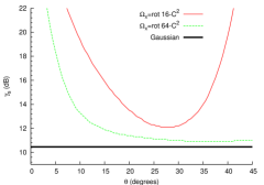
(a) The optimization of the rotation angle for complex symbols is shown.

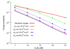
(b) The outage probabilities of the BF channel with complex inputs are shown.

Figure 9: The optimization of $\theta$ and the optimized outage probabilities are shown when complex symbols are transmitted. The transmitted rate is $R=1.8$ bpcu.

Note that, for $\Omega_{z}=16$-$\mathcal{C}^{2}$, the profile of the rotation angle $\theta$, and so the optimum rotation angle, is the same as for $\Omega_{z}=4$-$\mathcal{R}^{2}$ and $R=0.9$ bpcu. This can be explained as follows. When $\mathcal{R}\{\mathbf{z}\}$ and $\mathbb{I}\{\mathbf{z}\}$ are drawn from the same real-valued constellation $\Psi_{z}$, then $\mathbf{z}$ belongs to a constellation $\Omega_{z}=\Psi_{z}+j\Psi_{z}$. Consequently, $\mathbf{x}$ belongs to a constellation $\Omega_{x}=\Psi_{x}+j\Psi_{x}$, where $\Psi_{x}$ is obtained by applying the precoding matrix $P$ to the constellation $\Psi_{z}$. From the chain rule of mutual information [5], we obtain

$$I_{\Omega_{x}}\left(\gamma\right)=2I_{\Psi_{x}}\left(\frac{\gamma}{2}\right).$$ (21)

Hence, the precoding matrix $P$ that is optimum for a real-valued constellation $\Psi_{z}$ and rate $R$ is also optimum for a complex constellation $\Omega_{z}=\Psi_{z}+j\Psi_{z}$ and rate $2R$. The corresponding SNR for the complex constellation is $3$ dB higher than for the real-valued constellation. For $\Omega_{z}=16$-$\mathcal{C}^{2}$ and $R=1.8$ bpcu, the corresponding real-valued constellation is $\Psi_{z}=4$-$\mathcal{R}^{2}$. Therefore, the profiles in Figs. 9(a) and 7 are the same for both constellations, except for an upward translation of $3$ dB.

We also tested the performance for higher spectral efficiencies. Consider for example a system requiring a spectral efficiency of $R=3.6$ bpcu. Here, the same techniques can be used. First, $\Omega_{z}=256$-$\mathcal{C}^{2}$ (16-QAM$\times$16-QAM, $R_{c}=0.9$) is optimized, followed by $\Omega_{z}=1024$-$\mathcal{C}^{2}$ (32-QAM$\times$32-QAM , $R_{c}=0.72$). The results are given in Fig. 10. The same observations hold as for the previous numerical results.

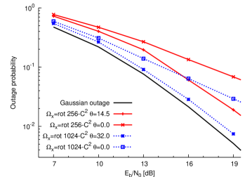
Figure 10: Outage probabilities of the BF channel with input $\Omega_{z}=256$-$\mathcal{C}^{2}$ and $\Omega_{z}=1024$-$\mathcal{C}^{2}$. The spectral efficiency is $R=3.6$ bpcu.

VII-B Numerical results for $B=3$

When $B=3$, $\mathcal{O}=\theta_{1}$ (see Eq. (8)), and the optimization criterion for the upper bound on the outage probability is to find $\theta_{1}$ so that $I_{\mathcal{S}_{\textrm{p}}}^{-1}(\theta_{1},BR)$ is minimized. Next, a constellation expansion is performed to further minimize the upper bound as well as the lower bound on the outage probability.

We aim to transmit $R=0.9$ bpcu. We construct constellations $\Omega_{z}$ that are invariant to a cyclic shift of the components of the constellation points. Hence, the constellations are invariant to a rotation of $2\pi/3$ with respect to the bisector $(1,1,1)$ (this can be verified by evaluating $P$ in Eq. (8) for this rotation angle). An example of such constellations are the Cartesian products of three identical one-dimensional constellations, such as $8$-$\mathcal{R}^{3}=$(BPSK$)^{3}$ (constellation points are corners of a cube) and $64$-$\mathcal{R}^{3}=(4$-PAM$)^{3}$ (constellation points are the corners of four nested cubes). More sophisticated constellations can also be considered. For example, $16$-$\mathcal{R}^{3}$ can be constructed by considering 5 sets of three constellation points $\{(a_{j},b_{j},c_{j}),(b_{j},c_{j},a_{j}),(c_{j},a_{j},b_{j})\}$ for $j=1,\ldots,\ldots,5$, and adding a constellation point located on the bisector. To build the actual constellations, a few design parameters have to be specified, such as the distances between the planes perpendicular to the bisector, the radii of the circles containing three points of the constellation in the planes, how many points on the bisector are taken and how many points in groups of three are taken. These design parameters will impact on the final performance.

Because it is not the main topic of the paper, we will not elaborate on many different designs for the multidimensional constellations. We compare the performance of $8$-$\mathcal{R}^{3}$ ($R_{c}=0.9$), $16$-$\mathcal{R}^{3}$ ($R_{c}=0.675$) and $64$-$\mathcal{R}^{3}$ ($R_{c}=0.45$) in Fig. 11.

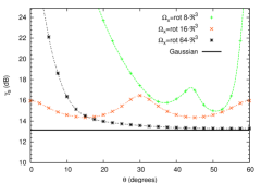
(a) The optimization of the rotation angle for $B=3$ is shown.

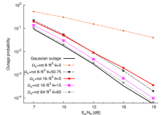
(b) The outage probabilities of the BF channel for $B=3$ are shown.

Figure 11: The optimization of $\theta_{1}$ and the optimized outage probabilities are shown for $B=3$. The transmitted rate is $R=0.9$ bpcu.

Note that the symmetry point in Fig. 11(a) is not $\theta_{1}=45$ degrees, as for $B=2$, but it is $60$ degrees. The $8$-$\mathcal{R}^{3}$ constellation is equal to the Cartesian product of three BPSK constellations and the $64$-$\mathcal{R}^{3}$ constellation is the Cartesian product of three 4-PAM constellations. For the $16$-$\mathcal{R}^{3}$ constellation, we chose to take a circle of three points in a plane containing the origin perpendicular to the bisector, and two circles with 6 points, each in a plane next to the first plane, perpendicular to the bisector. Finally the origin is also chosen as a constellation point. The rounded coordinates of the points of the constellation $\Omega_{z}$ are $\{(0.0,1.0,-1.0),(1.9,0.12,0.12),(1.3,-0.5,1.3),(0.5-1.3-1.3),(-1.9,-0.1,-0.1),(0,0,0)\}$ as well as the cyclic shifts of these coordinates.

VII-C Practical implications

The motivation for this work was to solve the theoretical problem of determining the optimal precoding matrix $P$ in terms of the outage probability for a given combination $\{R_{c},\Omega_{z}\}$ satisfying a target spectral efficiency $R$. Besides the theoretical relevance, the numerical results suggest a practical relevance because the impact of this optimization on the outage probability is significant in the case of large coding rates $R_{c}$ . This case might be preferred upon the case of small coding rates (and thus large constellation sizes for a given spectral efficiency $R$) because large constellation sizes complicates the system design (requiring a joint optimization of the constellation labeling and error-correcting code which is not trivial) and is sometimes even not allowed (e.g., $|\Omega_{z}|\leq 64$ in $4$G systems).

The consequences of our work on practical code design are as follows. The WER of a practical system is lower bounded by the outage probability (the lower bound is achievable). To minimize the WER, first its lower bound must be minimized. Therefore, the multidimensional constellation $\Omega_{z}$ and the rotation angle interval for the practical code should be taken as obtained in this work. Next, the labelling, the rotation angle within the rotation angle interval obtained in this paper, and the error-correcting code must be determined. The last three optimizations are the topics of another work [6], but it is important to understand that these optimizations are based on what is presented in this paper. In Fig. 12, we show for $B=2$ and $R=0.9$ bpcu that the optimized outage probability can be approached very closely by the WER of a practical system.

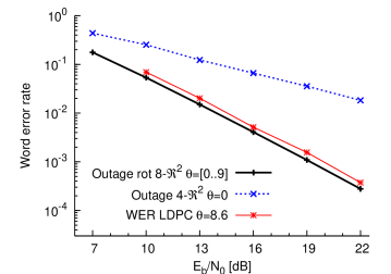
Figure 12: The optimized outage probability can be approached very closely by the WER of a practical error-correcting code. The block length is $N=5000$, but the results are valid for all block lengths (tested for $N=2000$ and $N=10000$).

VIII Conclusions

We have studied the effect of linear precoding on the outage probability of block fading channels. We have analyzed the outage boundaries in the fading space and established outer and inner boundaries with simple shapes which yield an easy optimization of the outage probability for a discrete constellation, for an arbitrary number of blocks in the fading channel, real-valued or complex constellations, low or high spectral efficiency. The combination of a constellation expansion and an optimized precoding matrix, has shown to be sufficient to closely approach the outage probability corresponding to an i.i.d. Gaussian input alphabet. With this work, the practical code performance can be optimized by admitting the parameters obtained here.

References

- [1] D. Bayer-Fluckiger, F. Oggier, E. Viterbo, “New algebraic constructions of rotated -lattice constellations for the Rayleigh fading channel ,” IEEE Trans. on Inf. Theory, vol. 50, no. 4, pp. 702-714, 2004.
- [2] E. Biglieri, J. Proakis, and S. Shamai, “Fading channels: information-theoretic and communications aspects,” IEEE Trans. on Inf. Theory, vol. 44, no. 6, pp. 2619-2692, Oct. 1998.
- [3] J.J. Boutros and E. Viterbo, “Signal space diversity: a power- and bandwidth-efficient diversity technique for the Rayleigh fading channel,” IEEE Trans. on Inf. Theory, vol. 44, no. 4, pp. 1453-1467, July 1998.
- [4] J.J. Boutros, A. Guillén i Fàbregas, and E. Calvanese, “Analysis of coding on non-ergodic block fading channels,” Allerton Conf. on Communication and Control, Illinois, 2005.
- [5] T.M. Cover and J.A. Thomas, Elements of Information Theory, New York, Wiley, 2006.
-
[6]
D. Duyck, J.J. Boutros, and M. Moeneclaey,
“Precoding for Word Error Rate Minimization of LDPC Coded Modulation on Block Fading Channels,”
Accepted for publication at the IEEE Trans. on Wir. Comm., April 2012, Download from telin.ugent.be/
~dduyck/publications/TWCOM_prec.pdf. - [7] D. Duyck, J.J. Boutros, and M. Moeneclaey, “Low-Density Graph Codes for Slow Fading Relay Channels,” IEEE Trans. on Inf. Theory, vol. 57, no. 7, July 2011.
- [8] D. Duyck, D. Capirone, C. Hausl, and M. Moeneclaey, “Design of Diversity-Achieving LDPC Codes for H-ARQ with Cross-Packet Channel Coding,” Personal Indoor Mobile Radio Communications (PIMRC), Istanbul, Turkey, Sept. 2010.
- [9] D. Duyck, J.J. Boutros, and M. Moeneclaey, “Rotated Modulations for Outage Probability Minimization: a fading space approach,” ISIT (Intern. Symp. on Inf. Theory), Texas, June 2010.
- [10] A. Guillén i Fàbregas, Concatenated codes for block-fading channels, Ph.D. thesis, EPFL, June 2004.
- [11] A. Guillén i Fàbregas and G. Caire, “Coded modulation in the block-fading channel: coding theorems and code construction,” IEEE Trans. on Inf. Theory, vol. 52, no. 1, pp. 91-114, Jan. 2006.
- [12] A. Guillén i Fàbregas and G. Caire, “Multidimensional coded modulation in block-fading channels,” IEEE Trans. on Inf. Theory, vol. 54, no. 5, pp. 2367-2372, 2008.
- [13] N. Gresset, J.J. Boutros, and L. Brunel, “Optimal linear precoding for BICM over MIMO channels,” International Symposium on Information Theory (ISIT), Chicago, Illinois, July 2004.
- [14] N. Gresset, L. Brunel, and J.J. Boutros, “Space-time coding techniques with bit interleaved coded modulation over block-fading MIMO channels,” IEEE Trans. on Inf. Theory, vol. 54, no. 5, pp. 2156-2178, May 2008.
- [15] D. Guo, S. Shamai, and S. Verdú, “Mutual information and minimum mean-square error in Gaussian channels,” IEEE Trans. on Inf. Theory, vol. 51, no. 4, pp. 1261-1282, Apr. 2005.
- [16] C. Hausl and A. Chindapol, “Hybrid ARQ with Cross-Packet Channel Coding,” IEEE Comm. Letters, vol. 11, no. 5, pp. 434-436, May 2007.
- [17] E.A. Jorswieck and H. Boche, “Outage probability in multiple antenna systems,” Eur. Trans. Telecomm., 18: 217 233.
- [18] R. Knopp and P.A. Humblet, “On coding for block fading channels,” IEEE Trans. on Inf. Theory, vol. 46, no. 1, pp. 189-205, Jan. 2000.
- [19] G.M. Kraidy, N. Gresset, and J.J. Boutros, “Information theoretical versus algebraic constructions of linear unitary precoders for non-ergodic multiple antenna channels,” Canadian Workshop on Information Theory, Montreal, Canada, June 2005.
- [20] J.N. Laneman, D. Tse, and G.W. Wornell, “Cooperative diversity in wireless networks: Efficient protocols and outage behavior,” IEEE Trans. Inf. Theory, vol. 50, no. 12, pp. 3062-3080, Dec. 2004.
- [21] A. Lozano, A. M. Tulino, and S. Verdú, “Optimum power allocation for parallel Gaussian channels with arbitrary input distributions,” IEEE Trans. on Inf. Theory, vol. 52, no. 7, pp. 3033 3051, July 2006.
- [22] E. Malkamaki and H. Leib, “Evaluating the performance of convolutional codes over block fading channels,” IEEE Trans. on Inf. Theory, vol. 45, no. 5, pp. 1643-1646, Jul. 1999.
- [23] S.K. Mohammed, E. Viterbo, Y. Hong, and A. Chockalingam, “Precoding by Pairing Subchannels to Increase MIMO Capacity with Discrete Input Alphabets,” IEEE Trans. on Inf. Theory, vol. 57, no. 7, pp. 4156-4169, July 2011.
- [24] S.K. Mohammed, E. Viterbo, Y. Hong, and A. Chockalingam, “MIMO Precoding with X- and Y-Codes,” IEEE Trans. on Inf. Theory, vol. 57, no. 6, pp. 3542-3566, June 2011.
- [25] L.H. Ozarow, S. Shamai, and A.D. Wyner, “Information theoretic considerations for cellular mobile radio,” IEEE Trans. on Vehicular Technology, vol. 43, no. 2, pp. 359-379, May 1994.
- [26] F. Pérez-Cruz, M.R.D. Rodrigues, and S. Verdú, “Optimal precoding for Digital Subscriber Lines,” in Proc. Intern. Conf. on Comm. (ICC), pp. 1200-1204, Beijing, China, May 2008.
- [27] F. Pérez-Cruz, M.R.D. Rodrigues, and S. Verdú, “MIMO Gaussian Channels With Arbitrary Inputs: Optimal Precoding and Power Allocation,” IEEE Trans. on Inf. Theory, vol. 56, no. 3, pp. 1070-1084, March 2010.
- [28] J.G. Proakis, “Digital Communications,” McGraw-Hill, 4th ed., 2000.
- [29] A. Sendonaris, E. Erkip, and B. Aazhang, “User cooperation diversity-Part I: System description,” IEEE Trans. Commun., vol. 51, no. 11, pp. 1927-1938, Nov. 2003, DOI: 10.1109/TCOMM.2003.818096.
- [30] A. Sendonaris, E. Erkip, and B. Aazhang, “User cooperation diversity-Part II: Implementation aspects and performance analysis,” IEEE Trans. Commun., vol. 51, no. 11, pp. 1939-1948, Nov. 2003.
- [31] I.E. Telatar, “Capacity of multi-antenna Gaussian channels,” Europ. Trans. on Telecomm., vol. 10, pp. 585-595, Nov./Dec. 1999.
- [32] D.N.C. Tse and P. Viswanath, Fundamentals of Wireless Communication, Cambridge University Press, May 2005.