Excitation spectrum and high energy plasmons in single- and multi-layer graphene

Abstract

In this paper we study the excitation spectrum of single- and multi-layer graphene beyond the Dirac cone approximation. The dynamical polarizability of graphene is computed using a full $\pi$-band tight-binding model, considering the possibility of inter-layer hopping in the calculation. The effect of electron-electron interaction is considered within the random phase approximation. We further discuss the effect of disorder in the spectrum, which leads to a smearing of the absorption peaks. Our results show a redshift of the $\pi$-plasmon dispersion of single-layer graphene with respect to graphite, in agreement with experimental results. The inclusion of inter-layer hopping in the kinetic Hamiltonian of multi-layer graphene is found to be very important to properly capture the low energy region of the excitation spectrum.

I Introduction

One of the main issues in the understanding of the physics of graphene is the role played by electron-electron interaction.For a recent review on electron-electron interaction in graphene, see et al. (2010) Several collective modes as low and high energy plasmons, as well as plasmarons, are a consequence of electronic correlations and have been measured in this material. The high energy $\pi$-plasmons have been observed in electron energy-loss spectroscopy (EELS),Kramberger et al. (2008); Eberlein et al. (2008); Gass et al. (2008) inelastic X-ray scattering (IXS)Reed et al. (2010) or optical conductivity.Mak et al. (2011) Recently, a plasmaron mode (which is a result of coupling between electrons and plasmons) has been measured in angle-resoved photoemission spectroscopy (ARPES).Bostwick et al. (2010)

At low energies, long range Coulomb interaction leads, in doped graphene, to a gapless plasmon mode which disperses as $\omega_{pl}\sim\sqrt{q}$,Liu et al. (2008) and which can be described theoretically within the random phase approximation (RPA).Shung (1986); Wunsch et al. (2006); Hwang and Sarma (2007); Polini et al. (2008); Pyatkovskiy (2009); Gamayun (2011) The low energy linear dispersion relation of graphene is at the origin of a new series of collective modes predicted for this material and which do not exist for other two-dimensional electron gases (2DEG), as inter-valley plasmonsTudorovskiy and Mikhailov (2010) or linear magneto-plasmons,Roldán et al. (2009) which can be described within the RPA as well. For undoped graphene, the inclusion of ladder diagrams in the polarization can lead to a new class of collective modesGangadharaiah et al. (2008) as well as to an excitonic instability.Khveshchenko (2001); Aleiner et al. (2007); Gamayun et al. (2009); Wang et al. (2010); González (2010)

However, much less is known about the high energy $\pi$-plasmon which, in the long wavelength limit, has an energy of the order of 5-6 eV, and which is due to the presence of Van Hove singularities in the band dispersion. For single-layer graphene (SLG), this mode has been studied by Stauber et al.Stauber et al. (2010) and by Hill et al.Hill et al. (2009) in the RPA. Yang et al. have included excitonic effects and found a redshift of the absorption peak,Yang et al. (2009) leading to a better agreement with the experimental results.Eberlein et al. (2008) Here we extend those previous works and study the excitation spectrum of SLG and multi-layer graphene (MLG) from a tight-binding model on a honeycomb lattice. By means of the Kubo formula, the non-interacting polarization function $\Pi(\mathbf{q},\omega)$ is obtained from the numerical solution of the time-dependent Schrödinger equation. Coulomb interactions are considered in the RPA, the validity of which is discussed. We also consider the effect of disorder in the system, which lead to a considerable smearing of the Van Hove singularities in the spectrum. Our results show a redshift of the $\pi$-plasmon mode in graphene with respect to graphite, as it has been observed in the experiments.Kramberger et al. (2008); Eberlein et al. (2008) Furthermore, the inclusion of inter-layer hopping is found to be very important to capture the low energy region of the spectrum in MLG.

The paper is organized as follows. In Sec. II we describe the method that we use to compute the dynamical polarization function of SLG and MLG. In Sec. III we give results for the excitation spectrum of SLG, considering the effect of disorder and electron-electron interaction. The spectrum of MLG is described in Sec. IV. In Sec. V we compare our results to recent experimental data. Our main conclusions are summarized in Sec. VI.

II Description of the method

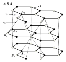
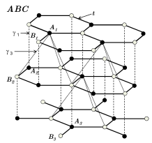
Figure 1: Atomic structure of ABA- and ABC-stacked multilayer graphene. The intra-layer ($t$) and inter-layer ($\gamma_{1}$ and $\gamma_{3}$) hopping amplitudes are considered, as explained in the text.

The tight-binding Hamiltonian of a MLG is given by

$$H=\sum_{l=1}^{N_{layer}}H_{l}+\sum_{l=1}^{N_{layer}-1}H_{l}^{\prime},$$ (1)

where $H_{l}$ is the Hamiltonian of the $l$’th layer of graphene,

$$H_{l}=-\sum_{<i,j>}(t_{l,ij}a_{l,i}^{\dagger}b_{l,j}+\mathrm{h.c})+\sum_{i}v_{l,i}c_{l,i}^{\dagger}c_{l,i},$$ (2)

where $a_{l,i}^{\dagger}$ ($b_{l,i}$) creates (annihilates) an electron on sublattice A (B) of the $l$’th layer, and $t_{l,ij}$ is the nearest neighbor hopping parameter. The second term of $H_{l}$ accounts for the effect of an on-site potential $v_{l,i}$, where $n_{l,i}=c^{\dagger}_{l,i}c_{l,i}$ is the occupation number operator. In the second term of the Hamiltonian Eq. (1), $H_{l}^{\prime}$ describes the hopping of electrons between layers $l$ and $l+1$. In nature there are two known forms of stable stacking sequence in bulk graphite, namely ABA (Bernal) and ABC (rhombohedral) stacking, and they are schematically shown in Fig. 1. For a MLG with an ABA stacking, $H_{l}^{\prime}$ is given by

$$H_{l}^{\prime}=-\gamma_{1}\sum_{j}\left[a_{l,j}^{\dagger}b_{l+1,j}+\mathrm{h.c.}\right]-\gamma_{3}\sum_{j,j^{\prime}}\left[b_{l,j}^{\dagger}a_{l+1,j^{\prime}}+\mathrm{h.c.}\right],$$ (3)

where the inter-layer hopping terms $\gamma_{1}$ and $\gamma_{3}$ are shown in Fig. 1. Thus, all the even layers ($l+1$) are rotated with respect to the odd layers ($l$) by $+120^{\circ}$. The difference between ABA and ABC stacking is that, the third layer(s) is rotated with respect to the second layer by $-120^{\circ}$ (then it will be exactly under the first layer) in ABA stacking, but by $+120^{\circ}$ in ABC stacking.Koshino (2010) In this paper we use the hopping amplitudes $t=3$ eV, $\gamma_{1}=0.4$ eV and $\gamma_{3}=0.3$ eV.Castro-Neto et al. (2009) The spin degree of freedom contributes only through a degeneracy factor and is omitted for simplicity in Eq. (1). In our numerical calculations, we use periodic boundary conditions in the plane ($XY$) of graphene layers, and open boundary conditions in the stacking direction ($Z$).

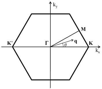
Figure 2: 2D Brillouin zone of SLG. For undoped graphene, the valence and conduction bands touch each other at the vertices of the hexagon, the so called Dirac points (K and K’). The Van Hove singularity lies at the M point, and we have defined $\theta$ as the angle between the wave-vector $q$ and the $k_{x}$-axis.

The dynamical polarization can be obtained from the Kubo formula Kubo (1957) as

$$\Pi\left(\mathbf{q},\omega\right)=\frac{i}{V}\int_{0}^{\infty}d\tau e^{i\omega\tau}\left\langle\left[\rho\left(\mathbf{q},\tau\right),\rho\left(-\mathbf{q},0\right)\right]\right\rangle,$$ (4)

where $V$ denotes the volume (or area in 2D) of the unit cell, $\rho\left(\mathbf{q}\right)$ is the density operator given by

$$\rho\left(\mathbf{q}\right)=\sum_{l=1}^{N_{layer}}\sum_{i}c_{l,i}^{\dagger}c_{l,i}\exp\left(i\mathbf{q\cdot r}_{l,i}\right),$$ (5)

and the average is taken over the canonical ensemble. For the case of the single-particle Hamiltonian, Eq. (4) can be written asYuan et al. (2010a)

$$\Pi\left(\mathbf{q},\omega\right)=-\frac{2}{V}\int_{0}^{\infty}d\tau e^{i\omega\tau}$$

$$\times\text{Im}\left\langle\varphi\right|n_{F}\left(H\right)e^{iH\tau}\rho\left(\mathbf{q}\right)e^{-iH\tau}\left[1-n_{F}\left(H\right)\right]\rho\left(-\mathbf{q}\right)\left|\varphi\right\rangle,$$

where $n_{F}\left(H\right)=\frac{1}{e^{\beta\left(H-\mu\right)}+1}$ is the Fermi-Dirac distribution operator, $\beta=1/k_{B}T$ where $T$ is the temperature and $k_{B}$ is the Boltzmann constant, and $\mu$ is the chemical potential. In the numerical simulations, we use units such that $\hbar=1$, and the average in Eq. (II) is performed over a random phase superposition of all the basis states in the real space, i.e.,Hams and De Raedt (2000); Yuan et al. (2010a)

$$\left|\varphi\right\rangle=\sum_{l,i}a_{l,i}c_{l,i}^{\dagger}\left|0\right\rangle,$$ (7)

where $a_{l,i}$ are random complex numbers normalized as $\sum_{l,i}\left|a_{l,i}\right|^{2}=1$. By introducing the time evolution of two wave functions

$$\left|\varphi_{1}\left(\mathbf{q,}\tau\right)\right\rangle = e^{-iH\tau}\left[1-n_{F}\left(H\right)\right]\rho\left(-\mathbf{q}\right)\left|\varphi\right\rangle,$$ (8)

$$\left|\varphi_{2}\left(\tau\right)\right\rangle = e^{-iH\tau}n_{F}\left(H\right)\left|\varphi\right\rangle,$$ (9)

we get the real and imaginary part of the dynamical polarization as

$$\text{Re}\Pi\left(\mathbf{q},\omega\right) = -\frac{2}{V}\int_{0}^{\infty}d\tau\cos(\omega\tau)~{}\text{Im}\left\langle\varphi_{2}\left(\tau\right)\left|\rho\left(\mathbf{q}\right)\right|\varphi_{1}\left(\tau\right)\right\rangle,$$

$$\text{Im}\Pi\left(\mathbf{q},\omega\right) = -\frac{2}{V}\int_{0}^{\infty}d\tau\sin(\omega\tau)~{}\text{Im}\left\langle\varphi_{2}\left(\tau\right)\left|\rho\left(\mathbf{q}\right)\right|\varphi_{1}\left(\tau\right)\right\rangle,$$

The Fermi-Dirac distribution operator $n_{F}\left(H\right)$ and the time evolution operator $e^{-iH\tau}$ can be obtained by the standard Chebyshev polynomial decomposition.Yuan et al. (2010a)

For the case of SLG, we will further compare the polarization function obtained from the Kubo formula Eq. (4), to the one obtained from the usual Lindhard function.Giuliani and Vignale (2005) Notice that this method can be used to calculate the optical conductivity of graphene beyond the Dirac cone approximation. Stauber et al. (2008); Yuan et al. (2010a) For pristine graphene, the dynamical polarization obtained from the Lindhard function using the full $\pi$-band tight-binding model isShung (1986); Hill et al. (2009); Stauber et al. (2010)

$$\Pi\left(\mathbf{q},\omega\right)=-\frac{g_{s}}{\left(2\pi\right)^{2}}\int_{BZ}d^{2}\mathbf{k}$$

$$\times\sum_{s,s^{\prime}=\pm}f_{s\cdot s^{\prime}}\left(\mathbf{k},\mathbf{q}\right)\frac{n_{F}\left[E^{s}\left(\mathbf{k}\right)\right]-n_{F}\left[E^{s^{\prime}}\left(\mathbf{k}+\mathbf{q}\right)\right]}{E^{s}\left(\mathbf{k}\right)-E^{s^{\prime}}\left(\mathbf{k}+\mathbf{q}\right)+\omega+i\delta},$$

where the integral is over the Brillouin zone, $g_{s}=2$ is the spin degeneracy, $E^{\pm}\left(\mathbf{k}\right)=\pm t\left|\phi_{\mathbf{k}}\right|-\mu$ is the energy dispersion with respect to the chemical potential, where

$$\phi_{\mathbf{k}}=1+2e^{i3k_{x}a/2}\cos\left(\frac{\sqrt{3}}{2}k_{y}a\right),$$ (12)

$a=1.42$Å  being the in-plane carbon-carbon distance, and the overlap between the wave-functions of the electron and the hole is given by

$$f_{\pm}\left(\mathbf{k},\mathbf{q}\right)=\frac{1}{2}\left(1\pm\text{Re}\left[e^{iq_{x}a}\frac{\phi_{\mathbf{k}}}{\left|\phi_{\mathbf{k}}\right|}\frac{\phi_{\mathbf{k+q}}^{\ast}}{\left|\phi_{\mathbf{k+q}}\right|}\right]\right).$$ (13)

In the RPA, the response function of SLG due to electron-electron interactions can be calculated as

$$\chi\left(\mathbf{q},\omega\right)=\frac{\Pi\left(\mathbf{q},\omega\right)}{\mathbf{1}-V\left(q\right)\Pi\left(\mathbf{q},\omega\right)},$$ (14)

where $V\left(q\right)=\frac{2\pi e^{2}}{\kappa q}$ is the Fourier component of the Coulomb interaction in two dimensions, in terms of the background dielectric constant $\kappa$, and

$$\mathbf{\varepsilon}\left(\mathbf{q},\omega\right)=\mathbf{1}-V\left(q\right)\Pi\left(\mathbf{q},\omega\right)$$ (15)

is the dielectric function of the system. We will be interested on the collective modes of the system, which are defined from the zeroes of the dielectric function [$\varepsilon(\mathbf{q},\omega)=0$]. The dispersion relation of the collective modes is defined from

$$\mathrm{Re}~{}\varepsilon(\mathbf{q},\omega_{pl})=1-V(q)\Pi(\mathbf{q},\omega_{pl})=0,$$ (16)

which leads to poles in the response function (14). The damping $\gamma$ of the mode is proportional to $\mathrm{Im}~{}\Pi(\mathbf{q},\omega_{pl})$, and it is given by

$$\gamma=\frac{\mathrm{Im}~{}\Pi(\mathbf{q},\omega_{pl})}{\left.\frac{\partial}{\partial\omega}\mathrm{Re}~{}\Pi(\mathbf{q},\omega)\right|_{\omega=\omega_{pl}}}.$$ (17)

For MLG, the response function is calculated as (we use $q_{z}=0$)Shung (1986)

$$\chi_{3D}\left(\mathbf{q},\omega\right)=\frac{\Pi_{3D}\left(\mathbf{q},\omega\right)}{\mathbf{1}-V\left(q\right)F\left(q\right)\Pi_{3D}\left(\mathbf{q},\omega\right)d},$$ (18)

where $d=3.35$Å  is the inter-layer separation. Because we use open boundary conditions in the stacking direction, we define the form factor $F\left(q\right)$ as

$$F\left(q\right)=\frac{1}{N_{layer}}\sum_{l,l^{\prime}=1}^{N_{layer}}e^{-q\left|l-l^{\prime}\right|d}.$$ (19)

The expression (18) assumes that the polarization of each layer is the same, and it is exact in two different limits: bilayer graphene and graphite. Notice that a similar effective form factor has been used to study the loss function of multiwall carbon nanotubes.Shyu and Lin (2000) Eq. (19) coincides with the commonly used form factor for a multi-layer system with an infinite number of layers:Das Sarma and Quinn (1982)

$$F\left(q\right)|_{N_{layer}\rightarrow\infty}=\sum_{l^{\prime}}e^{-q\left|l-l^{\prime}\right|d},$$ (20)

where in this last case the periodicity ensures that $F\left(q\right)$ is independent of layer index $l$, with the asymptotic behavior $F(q)=\sinh(qd)/[\cosh(qd)-1]$.Das Sarma and Quinn (1982)

A crucial issue is the value of the dielectric constant $\kappa$ for each of the cases considered, because it encodes the screening due to high energy ($\sigma$) bands which are not explicitly considered in our calculation. A good estimation for it can be obtained from the expressionWehling et al. (2011)

$$\kappa\left(\mathbf{q}\right)=\frac{\kappa_{1}+1-\left(\kappa_{1}-1\right)e^{-qL}}{\kappa_{1}+1+\left(\kappa_{1}-1\right)e^{-qL}}\kappa_{1},$$ (21)

where $\kappa_{1}\approx 2.4$ is the dielectric constant of graphite, $L=d_{m}+\left(N_{layer}-1\right)d$ is the total height of the multi-layer system in terms of the number of layers $N_{layer}$ and the height of a monolayer graphene $d_{m}\approx 2.8$ Å. As expected, Eq. (21) gives $\kappa=1$ for SLG at $q\rightarrow 0$ and $\kappa=\kappa_{1}$ for graphite.

We notice that the accuracy of the numerical results for the polarization function Eq. (II) is mainly determined by three factors: the time interval of the propagation, the total number of time steps, and the size of the sample. The maximum time interval of the propagation in the time evolution operator is determined by the Nyquist sampling theorem. This implies that employing a sampling interval $\Delta\tau=\pi/\max_{i}\left|E_{i}\right|$, where $E_{i}$ are the eigenenergies, is sufficient to cover the full range of energy eigenvalues. On the other hand, the accuracy of the energy eigenvalues is determined by the total number of the propagation time steps ($N_{\tau}$) that is the number of the data items used in the fast Fourier transform (FFT). Eigenvalues that differ less than $\Delta E=\pi/N_{\tau}\Delta\tau$ cannot be identified properly. However, since $\Delta E$ is proportional to $N_{\tau}^{-1}$ we only have to double the length of the calculation to increase the accuracy by the same factor. The statistic error of our numerical method is inversely proportional to the dimension of the Hilbert space,Hams and De Raedt (2000) and in our case (the single particle representation), it is the number of sites in the sample. A sample with more sites in the real space will have more random coefficients ($a_{l,i}$) in the initial state $\left|\varphi\right\rangle$, providing a better statistical representation of the superposition of all energy eigenstates.Yuan et al. (2010a)

Similar algorithm has been successfully used in the numerical calculation of the electronic structure and transport properties of single- and multi-layer graphene, such as the density of states (DOS), or dc and ac conductivities.Wehling et al. (2010); Yuan et al. (2010a, b) The main advantage of our algorithm is that different kinds of disorders and boundary conditions can be easily introduced in the Hamiltonian, and the computer memory and CPU time is linearly proportional to the size of the sample, which allows us to do the calculations on a sample containing tens of million sites.

III Excitation spectrum of single-layer graphene

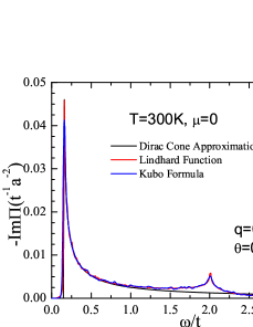
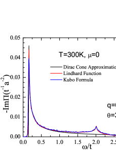
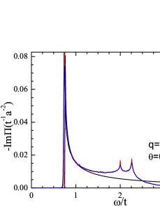
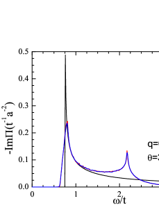
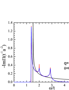
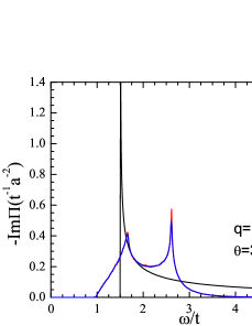
Figure 3: (Color online) $-\mathrm{Im}~{}\Pi(\mathbf{q},\omega)$ for SLG in the clean limit for different values of wave-vector $\mathbf{q}$. Plots (a), (c) and (e) correspond to a wave-vector $\mathbf{q}$ along $\Gamma$-K, whereas (b), (d) and (f) are of a $\mathbf{q}$ parallel to the $\Gamma$-M direction. The angle $\theta$ is defined in Fig. 2. In the numerical integration of Lindhard function in Eq. (II), we use $2\times 10^{8}$ Monte Carlo points (k) in the first Brilion. The sample size of SLG used in the numerical calculation of Kubo formula in Eq. (II) is $4096\times 4096.$

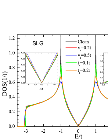
Figure 4: (Color online) Density of states for SLG considering different kind of disorder. The left inset shows a zoom of the DOS near the Dirac point ($E=0$), whereas the right hand side inset shows the disorder broadening of the Van Hove singularity at $E=t$. The numerical method used in the calculation of DOS is discribed in Ref. Yuan et al., 2010a, and the sample size of SLG is $4096\times 4096.$

The particle-hole excitation spectrum is the region of the energy-momentum space which is available for particle-hole excitations. For non-interacting electrons, it is defined as the region where $\mathrm{Im}~{}\Pi(\mathbf{q},\omega)$, as given by Eq. (4) or (II), is non-zero.Giuliani and Vignale (2005) The linear low energy dispersion relation of graphene as well as the possibility for inter-band transitions lead to a rather peculiar excitation spectrum for SLG as compared to the one of a two-dimensional electron gas (2DEG) with a parabolic band dispersion.Roldán et al. (2010) Here we focus on undoped graphene ($\mu=0$), for which only inter-band transitions are allowed. In Fig. 3 we plot $\mathrm{Im}~{}\Pi(\mathbf{q},\omega)$ for different wave-vectors at $T=300K$ (which is the temperature that we will use from here on in our results). The first thing one observes is the good agreement between the results obtained from the Kubo formula Eq. (4), as compared to Lindhard function Eq. (II), what proofs the validity of our numerical method. Furthermore, for the small wave-vector used in Fig. 3(a)-(b), the results are well described by the Dirac cone approximation,Wunsch et al. (2006); Hwang and Sarma (2007) but only at low energies, around $\omega\sim v_{\mathrm{F}}q$, where $v_{\mathrm{F}}=3at/2$ is the Fermi velocity near the Dirac points. In particular, the continuum approximation cannot capture the peaks of $\mathrm{Im}\Pi(\mathbf{q},\omega)$ around $\omega\approx 2t$. These peaks are related to particle-hole excitations between states of the valence band with energy $E\approx-t$ and states of the conduction band with energy $E\approx t$, which contribute to the polarization with a strong spectral weight due to the enhanced density of states at the Van Hove singularities of the $\pi$-bands (see Fig. 4).

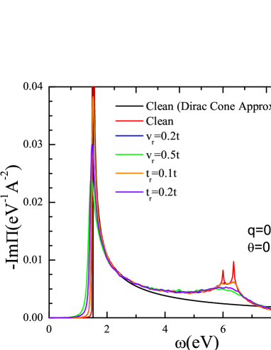
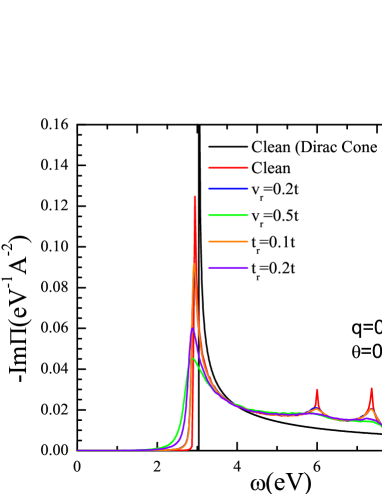
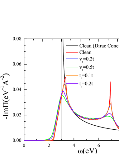
Figure 5: (Color online) $-\mathrm{Im}~{}\Pi(\mathbf{q},\omega)$ for different kinds of disorder and for different values and orientation of the wave-vector $\mathbf{q}$. In all the plots, the results using the Kubo formula Eq. (4) are compared to the Dirac cone approximation. The sample size of SLG is $4096\times 4096.$

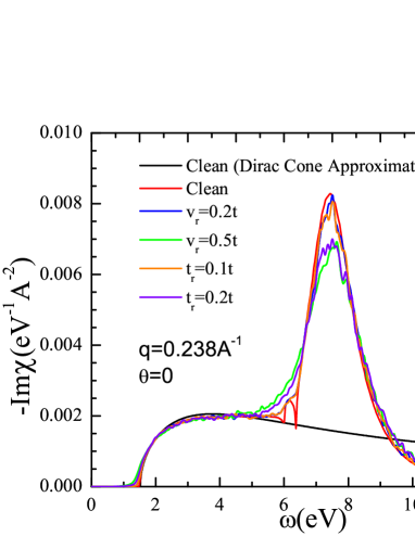
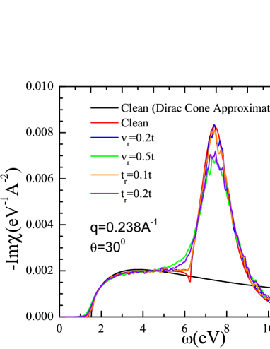
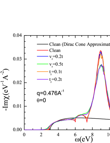
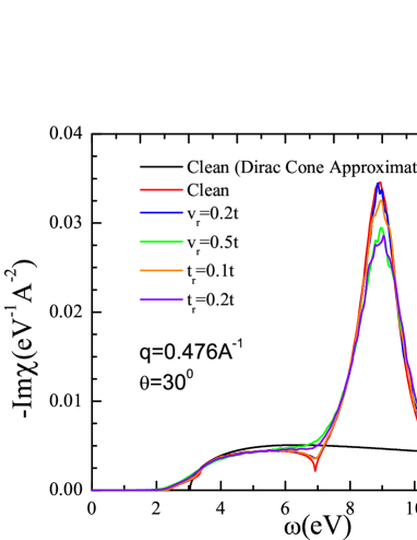
Figure 6: (Color online) $-\mathrm{Im}~{}\chi(\mathbf{q},\omega)$ for the same values of $\mathbf{q}$ and disorder as in Fig. 5.

Second, for larger wave-vectors [Figs. 3(c)-(f)] one observes strong differences in the spectrum depending on the orientation of $\mathbf{q}$, effect which has been discussed previously.Stauber et al. (2010); Stauber and Gómez-Santos (2010) If $\mathbf{q}$ is along the $\Gamma$-K direction, there is a splitting of the peak associated to the Van Hove singularity at $\omega\sim 2t$. At low energies, we also observe a finite contribution to the spectral weight to the left of the $\omega\approx v_{\mathrm{F}}q$ peak for momenta along the $\Gamma$-M direction [plots Figs. 3(d) and (f)]. Finally, trigonal warping effects are important as we increase the magnitude of $|\mathbf{q}|$, due to the deviation of the band dispersion with respect to the linear cone approximation. As a consequence, the constant energy contours are not any more circles around the Dirac points, but present a triangular shape. The consideration of this effect leads to a redshift of the $\omega\approx v_{\mathrm{F}}q$ peak with respect to the Dirac cone approximation, as seen clearly in Fig. 3(e).

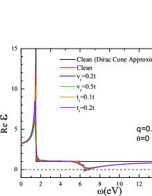
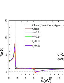
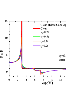
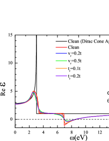
Figure 7: (Color online) $\mathrm{Re}~{}\varepsilon(\mathbf{q},\omega)$ for the same values of $\mathbf{q}$ and disorder as in Fig. 5 and 6.

Once we have discussed the clean case, we consider the effect of disorder on the excitation spectrum as explained in Sec. II. Two different kinds of disorder are considered: random local change of on-site potentials and random renormalization of the hopping, which correspond to the diagonal and off-digonal disorders in the single-layer Hamiltonian Eq. (2), respectively. The former acts as a chemical potential shift for the Dirac fermions, i.e., shifts locally the Dirac point, and the later rises from the changes of distance or angles between the $p_{z}$ orbitals. In Fig. 4 we show the DOS of SLG for different kinds and magnitudes of disorder. The DOS for clean graphene has been plotted by using the analytical expression given in Ref. Hobson and Nierenberg, 1953. The DOS of the disordered systems are calculated by Fourier transform of the time-dependent correlation functions Yuan et al. (2010a)

$$\rho\left(\varepsilon\right)=\frac{1}{2\pi}\int_{-\infty}^{\infty}e^{i\varepsilon t}\left\langle\varphi\right|e^{-iHt}\left|\varphi\right\rangle dt,$$ (22)

with the same initial state $\left|\varphi\right\rangle$ defined in Eq. (7). As shown in Ref. Yuan et al., 2010a, the result calculated from a SLG with $4096\times 4096$ lattice sites matches very well with the analytical expression, and here we use the same sample size in the disordered systems. We consider that the on-site potential $v_{i}$ is random and uniformly distributed (independently on each site $i$ ) between $-v_{r}$ and $+v_{r}$. Similarly, the in-plane nearest-neighbor hopping $t_{ij}$ is random and uniformly distributed (independently on sites $i,j$) between $t-t_{r}$ and $t+t_{r}$. The main effect is a smearing of the Van Hove singularity at $E=t$, as observed in the right hand side inset of Fig. 4.

The effect of disorder is also appreciable in the non-interacting excitation spectrum of the system, as shown by Fig. 5. A broadening of the $\omega\approx v_{\mathrm{F}}q$ and $\omega\approx 2t$ peaks is observed in all the cases. Furthermore, disorder leads to a slight but appreciable redshift of the peaks with respect to the clean limit. This effect is more important for higher wave-vectors, as it can be seen in Fig. 5(c)-(d). Finally, the disorder broadening of the peaks leads in all the cases to a transfer of spectral weight to low energies (below $\omega=v_{\mathrm{F}}q$), as it is appreciable in Fig. 5(a)-(d).

The next step is to consider both, disorder and electron-electron interaction in the system. In the RPA, the response function is calculated as in Eq. (14). The results are shown in Fig. 6, where $-\mathrm{Im}~{}\chi(\mathbf{q},\omega)$ is plotted for the same wave-vectors and disorder used in Fig. 5. We observe that the Dirac cone approximation (black line) captures well the low energy region of the spectrum. However, the large peak at $\omega\sim 2t$ cannot be captured by the continuum approximation. They are due to a plasmon mode associated to transitions between electrons in the saddle points of the $\pi$-bands. Strictly speaking, those modes cannot be considered as fully coherent collective modes, as for example, the low energy $\sqrt{q}$-plasmon which is present in doped graphene.Shung (1986) For doped graphene, the acoustic $\sqrt{q}$-plasmon is undamped above the threshold $\omega=v_{\mathrm{F}}q$ until it enters the inter-band particle-hole continuum, when it starts to be damped and decays into electron-hole pairs. However, the $\pi$-plasmon, although it corresponds to a zero of the dielectric function as it can be seen in Fig. 7, it is a mode which lies inside the continuum of particle-hole excitations: $-\mathrm{Im}~{}\Pi(\mathbf{q},\omega_{pl})>0$ at the $\pi$-plasmon energy $\omega_{pl}$, and the mode will be damped even at $q\rightarrow 0$. In any case, it is a well defined mode which has been measured experimentally for SLG and MLG.Kramberger et al. (2008); Eberlein et al. (2008); Gass et al. (2008); Reed et al. (2010); Mak et al. (2011) Coming back to our results, notice that the height of the peaks is reduced when the effect of disorder is considered, although the position is unaffected by it. For small wave-vectors, this mode is highly damped due to the strong spectral weight of the particle-hole excitation spectrum at this energy, as seen e.g. by the peak of $-\mathrm{Im}~{}\Pi(\mathbf{q},\omega)$ at $\omega=2t$ in Fig. 3(a)-(b). The position of the collective modes can be alternatively seen by the zeroes of the dielectric function Eq. (16), which is shown in Fig. 7. Notice that the Dirac cone approximation (solid black lines in Fig. 7) is completely insufficient to capture this high energy $\pi$-plasmon, which predicts always a finite $\mathrm{Re}~{}\varepsilon(\mathbf{q},\omega)$. As for the polarization, we see that disorder lead to an important smearing of the singularities of the dielectric function, as seen in Fig. 7. Finally, we mention that the application of our method to even higher wave-vectors and energies as the ones considered in the present work, should be accompanied by the inclusion of local field effects (LFE) in the dielectric function, which are related to the periodicity of the crystalline lattice.Adler (1962) In fact, for SLG and for wave-vectors along the zone boundary between the M and the K points of the Brillouin zone (see Fig. 2), the inclusion of LFEs leads to a new optical plasmon mode at an energy of 20-25 eV.Pellegrino et al. (2010)

IV Excitation spectrum for multi-layer graphene

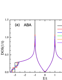
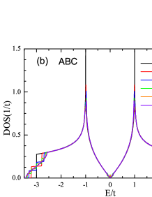
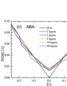
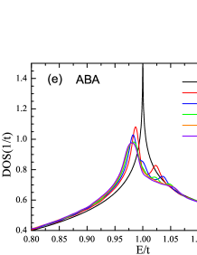
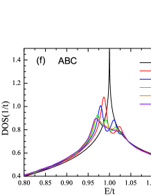
Figure 8: (Color online) (a,b) Density of states of ABA- (left panels) and ABC-stacked (right panels) multilayer graphene. A zoom of the DOS around the Dirac point ($E=0$) is shown in (c,d), and around the Van Hove singularity ($E=t$) is shown in (e,f). The sample sizes of each layer in MLG are: $4096\times 4096$ atoms in bilayer; $3200\times 3200$ in trilayer; $2048\times 2048$ in 5 layers; $1600\times 1600$ in 10 layers and $800\times 800$ in 50 layers.

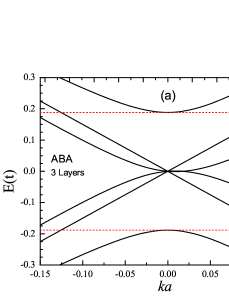
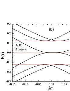
Figure 9: (Color online) Band structure of ABA- and ABC-stacked trilayer graphene. Left panel: the red dashed lines indicate the position of the jump in DOS of ABA-stacked trilayer graphene at $\left|E\right|\approx 0.19t$. Right panel: the red dashed lines indicate position of the peaks in DOS of ABC-stacked trilayer graphene at $E=0$ and $\left|E\right|\approx 0.12t$.

In the following, we study the excitation spectrum and collective modes of MLG. For this, we consider not only the Coulomb interaction between electrons on different layers, but also the possibility for the carriers to tunnel between neighboring layers, as described in Sec. II. The importance of considering inter-layer hopping has been already shown in the study of screening properties of MLG.Guinea (2007) First, we see that the results are sensitive to the relative orientation between layers. In Fig. 8 we show the density of states for ABA- and ABC- stacked MLG (see Fig. 1 for details on the difference between those two orientations). As seen in Fig. 8(c)-(d), all the MLGs present a finite DOS at $E=0$, contrary to SLG which has a vanishing DOS at the Dirac point. The main difference between the two kinds of stacking is that for ABC there is a central peak together with a series of satellite peaks around $E=0$ [Fig. 8(d)], whereas for ABA the DOS follows closer the behavior of the SLG [Fig.8(c)]. The different structure in the DOS can be understood by looking at Fig. 9, where we show the low energy band structure of a trilayer graphene with ABA [Fig. 9(a)] and ABC [Fig. 9(b)] orientations. The different jumps and peaks in the DOS of Fig. 8(c)-(d) are associated to the regions of the band dispersion marked by the horizontal red lines of Fig. 9, the energy of which depends on the values of the tight-binding parameters associated to inter-layer tunneling ($\gamma_{1}$ and $\gamma_{3}$ in our case). In the two cases, we observe a splitting of the Van Hove peak, as seen in Fig. 8(e)-(f). Notice that when we have a high number of layers (e.g. above 10 layers), there is a weak effect on adding a new graphene sheet to the system, as it can be seen from the similar DOS between the 10- and the 50-layers cases of Fig. 8.

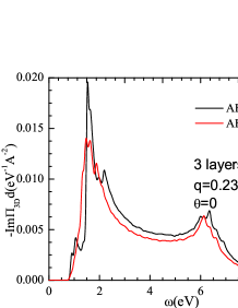
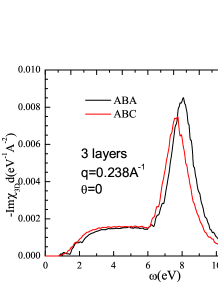
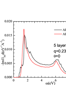
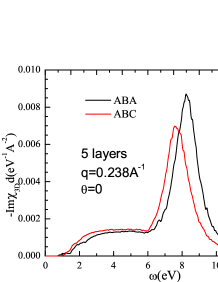
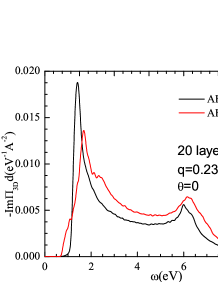
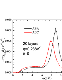
Figure 10: (Color online) Dynamical polarization and response function of ABA- and ABC-stacked multilayer graphene. The number of layers are 3 layers in (a,b), 5 layers in (c,d) and 20 layers in (e,f). The size of each layer is 3600$\times$3600 atoms for tri-layer (a,b); 3200$\times$3200 atoms for 5-layer samples (c,d), and 1600$\times$1600 atoms for 20-layer (e,f).

In Fig. 10 we show the non-interacting (left panels) and the RPA (right panels) polarization function of MLG, for systems made of 3, 5 and 20 layers, and for ABA- and ABC-stacking. For the spectrum in the absence of electron-electron interaction, as shown in Fig. 10(a), (c) and (e), one does not observe any specific difference in the two spectra apart from different intensities depending on the kind of stacking and on the number of layers considered for the calculation. On the other hand, the energy of the $\pi$-plasmon of ABC samples is redshifted with respect to the ABA-stacking. This can be see from the relative position of the peaks of $-\mathrm{Im}~{}\chi(\mathbf{q},\omega)$ in Fig. 10(b), (d) and (e). Also, notice that the separation between the two peaks grows with the number of layers, and for a 20-layers system, the difference can be of the order of 1 eV, as it can be seen in Fig. 10(f). In the following and unless we say the opposite, all the results will be calculated for the more commonly found ABA-stacking.

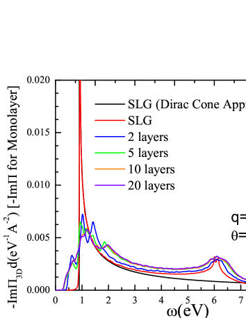
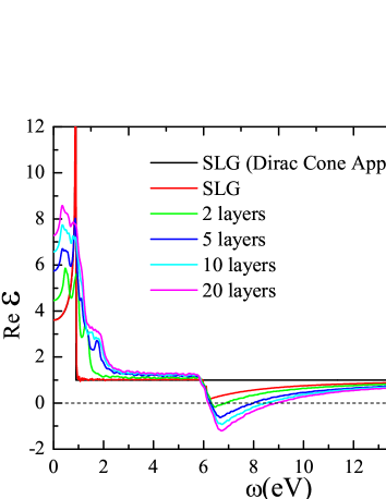
Figure 11: (Color online) (a) $\mathrm{Im}\Pi(\mathbf{q},\omega)$ for SLG and MLG. The results for SLG obtained from the Kubo formula Eq. (4) are compared to those obtained from the Lindhard function Eq. (II), and to the Dirac cone approximation. (b) $\mathrm{Re}~{}\varepsilon(\mathbf{q},\omega)$ for SLG and MLG, and comparison to the Dirac cone approximation, for the same value of $q$ as in (a).

For a more clear understanding about the evolution of the particle-hole excitation spectrum with the number of layers, we plot in Fig. 11(a) the imaginary part of $\Pi(\mathbf{q},\omega)$ for SLG and MLG of several number of layers, and compare the results to the polarization obtained using the Dirac cone approximation. It is very important to notice that multi-layer graphene presents some spectral weight at low energies as compared to graphene, which can be seen from the finite contribution of $\mathrm{Im}\Pi(\mathbf{q},\omega)$ that appears to the left of the big peak of the graphene polarizability at $\omega=v_{\mathrm{F}}q$ ($\sim 1$eV for the used parameters), in terms of the Fermi velocity near the Dirac point, $v_{\mathrm{F}}=3at/2$. This is due to the low energy parabolic-like dispersion of bilayer and multilayer graphene, as compared to the linear dispersion of single layer graphene, and it can only be captured by considering the inter-layer hopping contribution to the kinetic Hamiltonian Eq. (3). Furthermore, the spectrum presents a series of peaks for $\omega\approx v_{\mathrm{F}}q$, the number of which depends on the number of layers. This is due to the fact that as we increase the number of coupled graphene planes, the number of bands available for particle-hole excitations also grows leading to peaks at different energies for a given wave-vector.Zhang et al. (2008)

The difference between SLG and MLG is also relevant in the low energy region of the dielectric function, as it can be seen in Fig. 11(b). In fact, the $\omega\rightarrow 0$ limit of $\mathrm{Re}~{}\varepsilon(\mathbf{q},\omega)$ calculated within the RPA grows with the number of layers. Moreover, as we have discussed above, the zeroes of $\mathrm{Re}~{}\varepsilon(\mathbf{q},\omega)$ signal the position of collective excitations in the system (plasmons). In Fig. 11(b) we see that $\mathrm{Re}~{}\varepsilon(\mathbf{q},\omega)$, for the small wave-vector used, crosses 0 for MLG, revealing the existence of a solution of Eq. (16), but not so for SLG, as it was pointed out in Ref. Stauber et al., 2010. However, we emphasize that the very existence of solutions for the $\mathrm{Re}~{}\varepsilon(\mathbf{q},\omega)=0$ equation for MLG does not imply the existence of long-lived plasmon modes. In fact, as we have already discussed in Sec. III, these modes disperse within the continuum of particle-hole excitations [$\mathrm{Im}~{}\Pi(\mathbf{q},\omega_{pl})\neq 0$, where $\omega_{pl}$ is the solution of Eq. (16)], so they will be Landau damped and will decay into electron-hole pairs with a damping given by Eq. (17). Furthermore, we remember that for a given wave-vector, the energy of the mode is controlled by the background dielectric constant $\kappa$, as given by Eq. (21). For the systems under consideration, $\kappa$ changes between 1 (for SLG) and 2.4 (for graphite). The value of $\kappa$, together with the form factor Eq. (19) that takes into account inter-layer Coulomb interaction, fix the position of the modes in each case.

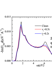
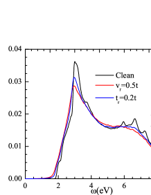
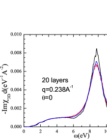
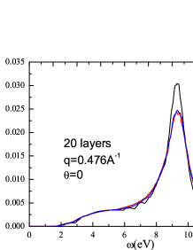
Figure 12: (Color online) Dynamical polarization and response function of ABA-stacked 20-layer graphene with disorders. The sample size of each layer is $1600\times 1600$.

The effect of disorder in MLG is considered in Fig. 12, where we show the polarization function of a 20-layer graphene system for different kinds of disorder. As in the SLG, we find that disorder leads to a slight redshift of the peaks of the non-interacting spectrum [Fig. 12(a) and (b)], together with a smearing of the peaks at $\omega\sim v_{\mathrm{F}}q$ and $\omega\sim 2t$. On the other hand, the interacting polarization function presents a reduction of the intensity of the plasmon peak due to disorder, as seen in Fig. 12(c) and (d), also in analogy with the SLG case.

V Discussion and comparison to experimental results

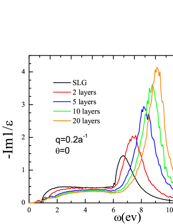
Figure 13: (Color online) Loss function $-\mathrm{Im}~{}1/\varepsilon(\mathbf{q},\omega)$ for SLG and MLG, which is proportional to the spectrum obtained by EEL experiments.Eberlein et al. (2008) We have used the same $q$ as in Fig. 11.

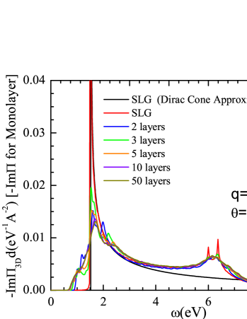
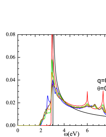
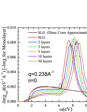
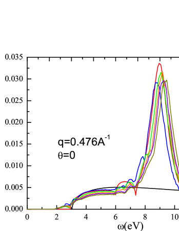
Figure 14: (Color online) Non-interacting polarization function $\mathrm{Im}\Pi(\mathbf{q},\omega)$ [plots (a) and (b)] and RPA response function $\mathrm{Im}\chi(\mathbf{q},\omega)$ [plots (c) and (d)] for SLG and MLG, for two different wave-vectors. The wave-vectors are chosen as in Ref. Reed et al., 2010.

In this section we compute quantities which are directly comparable to recent experimental results on SLG and MLG. We start by calculating the loss function $-\mathrm{Im}~{}1/\varepsilon(\mathbf{q},\omega)$, which is proportional to the spectrum measured by EELS. Our results, shown in Fig. 13, are in good agreement with the experimental data of Ref. Eberlein et al., 2008: as in the experiments, we observe a redshift of the plasmon peak as one decrease the number of layers, as well as an increase of the intensity with the number of layers. Notice that, due to finite size effects, there is an infra-red cutoff for the wave-vectors used in our calculations which prevents to reach the long wavelength limit. In Fig. 13 we show the results for the smallest wave-vector available, and we emphasize that the peaks will be further shifted to the left for smaller values of $q$. A further redshift of the peaks would be obtained beyond RPA, as it has been reported for single- and bilayer graphene, where excitonic effects have been included.Yang et al. (2009)

We have also used our method to study the IXS experiments of Reed et al.Reed et al. (2010) In Fig. 14(a)-(b) we plot the imaginary part of the non-interacting polarization function for SLG and MLG, for two values of $q$ similar to the ones used in Ref. Reed et al., 2010. As we have discussed in Sec. IV, inter-layer hopping leads to a finite contribution to the spectral weight in the low energy region of MLG as compared to the SLG spectrum. Notice that the number of peaks at this energy $\omega\approx v_{\mathrm{F}}q$ scales with the number of accessible bands and therefore, with the number of layers. We emphasize that this effect is not included by the usually employed approximation of considering MLG as a series of single-layers of graphene, only coupled via direct Coulomb interaction.Reed et al. (2010) Without the possibility of inter-layer hopping, the polarization function of graphene and graphite are, apart from some multiplicative factor, the same. As we have seen in Sec. IV, this simplification does not capture the low energy part of the spectrum, with some finite spectral weight due to low energy inter-band transitions between parabolic-like bands.

At an energy of the order of $\omega\approx 2t$ one observes the peak due to transitions between electrons from the Van Hove singularity of the occupied band to the singularity of the empty band. For SLG, the peak is split into two peaks if the wave-vector points in the $\Gamma$-K direction (as it is the case here), the separation of which increases with the modulus $q=q_{x}$. However the amplitude of these peaks is highly suppressed from SLG to MLG. Finally, one observes in Fig. 14(b) that for higher values of $q$, as the one used here, there is a redshift of the peak of $\mathrm{Im}~{}\Pi(\mathbf{q},\omega)$ at the energy $\omega\approx v_{\mathrm{F}}q$ with respect to the Dirac cone approximation. This is due to trigonal warping effects, which are beyond the continuum approximation. Summarizing, we find two effects that lead to a global contribution to the polarization at low energies: one is the contribution to the spectral weight due to inter-layer hopping in MLG, and the other is the redshift of the peaks at $\omega\approx v_{\mathrm{F}}q$ due to trigonal warping effects. Notice that, because we are studying the non-interacting polarization function, no excitonic effects are present in the results of Fig. 14(a)-(b).

Once the polarization function $\Pi(\mathbf{q},\omega)$ is known, we compute the response function $\chi(\mathbf{q},\omega)$ at the RPA level, as shown in Fig. 14(c)-(d). Again, we find a redshift of the position of the peaks as we decrease the number of layers. The different position of the peaks is due to the different contribution of inter-layer electron-electron interaction for each case, as well as to the different value of $\kappa$ as given by Eq. (21). Our results agree reasonably well with those of Ref. Reed et al., 2010.

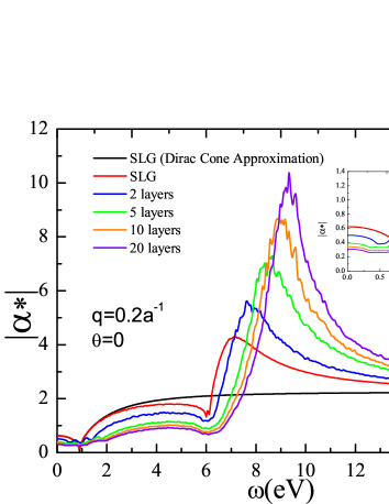
Figure 15: (Color online) Modulus of the screened fine structure constant $|\alpha^{*}|$, calculated from Eq. (23), for SLG and MLG of a different number of layers. The inset is a zoom for the more experimentally relevant $\omega\rightarrow 0$ region of the spectrum (see text). $|\alpha^{*}|\approx 0.6$ for SLG, whereas this value is highly reduced for MLG: $|\alpha^{*}|\approx 0.3$ for a 20-layers sample in our numerical calculation, which has a behavior very similar to graphite.

Finally, we calculate the renormalization of the fine structure constant $\alpha=e^{2}/v_{\mathrm{F}}$ due to dynamic screening associated to the inter-band transitions from the valence band. For this, and in analogy with Ref. Reed et al., 2010, we define

$$\alpha^{*}(\mathbf{q},\omega)=\frac{\alpha}{\varepsilon(\mathbf{q},\omega)}$$ (23)

The results for the modulus $|\alpha^{*}|$ for SLG and MLG are shown in Fig. 15. In this plot we have used the value of the Fermi velocity valid near the Dirac point, i.e., $v_{\mathrm{F}}=3at/2$. Therefore, we emphasize that these results should be reliable only at low energies. At $\omega\rightarrow 0$ and for the smallest wave-vector we can access ($q=0.2a^{-1}$), RPA predicts $|\alpha^{*}|\approx 0.6$ for SLG, which is considerably higher than the value estimated in Ref. Reed et al., 2010: $|\alpha^{*}|\approx 0.15$. However, the results that we obtain for MLG are much closer to this value: we find that $|\alpha^{*}|\approx 0.3$ for graphite, only slightly higher (a factor of 2) than the experimental results of Ref. Reed et al., 2010, which are actually obtained from graphite.

VI Conclusions

In conclusion, we have studied the excitation spectrum of single- and multi-layer graphene using a full $\pi$-band tight-binding model in the random phase approximation. We have found that, for MLG, the consideration of inter-layer hopping is very important to properly capture the low energy region ($\omega\sim v_{\mathrm{F}}q$) of the spectrum. This, together with trigonal warping effects, lead to a finite contribution to the spectral weight at low energies as well as a redshift of the peaks with respect to the Dirac cone approximation. We have also studied the high energy plasmons which are present in the spectrum of SLG and MLG at an energy of the order of $\omega\sim 2t\approx 6$eV and which are associated to the enhanced DOS at the Van Hove singularities of the $\pi$-bands. The energy of the $\pi$-plasmon depend also on the orientation between adjacent layers, and we find that, for a given wave-vector, the energy of the mode for ABC-stacked MLG is redshifted with respect to the corresponding energy of ABA ordering. This difference is higher as we increase the number of graphene layers of the system.

The effect of disorder has been considered by the inclusion of a random on-site potential and by a renormalization of the nearest neighbor hopping. Both kinds of disorder lead to a redshift of the $\omega\approx v_{\mathrm{F}}q$ and $\omega\approx 2t$ peaks of the non-interacting excitation spectrum and to a smearing of the Van Hove singularities. The position of the $\pi$-plasmons is unaffected by disorder, although the height of the absorption peaks is reduced as compared to the clean limit.

Finally, we have compared our results to some recent experiments. Our calculations for the loss function $\mathrm{Im}~{}1/\varepsilon(\mathbf{q},\omega)$ show a redshift of the SLG mode with respect to graphite, and compare reasonably well with experimental EELS data.Eberlein et al. (2008); Gass et al. (2008) Furthermore, we also obtain good agreement with the IXS results for the response function obtained in Ref. Reed et al., 2010. We obtain a static dielectric function which grows with the number of layers of the system. In the long wavelength and $\omega\rightarrow 0$ limit, the dynamically screened fine structure constant is found to be highly reduced from graphene to graphite. The value that we find for a MLG in the RPA, without considering any excitonic effects, is about two times larger than the one estimated in Ref. Reed et al., 2010 for graphene. More accurate results could be obtained going beyond single-band RPA,van Schilfgaarde and Katsnelson (2011) which is beyond the scope of this work.

VII Acknowledgement

The support by the Stichting Fundamenteel Onderzoek der Materie (FOM) and the Netherlands National Computing Facilities foundation (NCF) are acknowledged. We thank the EU-India FP-7 collaboration under MONAMI.

References

- For a recent review on electron-electron interaction in graphene, see et al. (2010) For a recent review on electron-electron interaction in graphene, see, V. Kotov, B. Uchoa, V. M. Pereira, A. H. Castro-Neto, and F. Guinea, (2010), arXiv:1012.3484 .
- Kramberger et al. (2008) C. Kramberger, R. Hambach, C. Giorgetti, M. H. Rümmeli, M. Knupfer, J. Fink, B. Büchner, L. Reining, E. Einarsson, S. Maruyama, F. Sottile, K. Hannewald, V. Olevano, A. G. Marinopoulos, and T. Pichler, Phys. Rev. Lett. 100, 196803 (2008).
- Eberlein et al. (2008) T. Eberlein, U. Bangert, R. R. Nair, R. Jones, M. Gass, A. L. Bleloch, K. S. Novoselov, A. Geim, and P. R. Briddon, Phys. Rev. B 77, 233406 (2008).
- Gass et al. (2008) M. H. Gass, U. Bangert, A. L. Bleloch, P. Wang, R. R. Nair, and A. Geim, Nature Nanotechnology 3, 676 (2008).
- Reed et al. (2010) J. P. Reed, B. Uchoa, Y. I. Joe, Y. Gan, D. Casa, E. Fradkin, and P. Abbamonte, Science 330, 805 (2010).
- Mak et al. (2011) K. F. Mak, J. Shan, and T. F. Heinz, Phys. Rev. Lett. 106, 046401 (2011).
- Bostwick et al. (2010) A. Bostwick, F. Speck, T. Seyller, K. Horn, M. Polini, A. H. MacDonald, and E. Rothenberg, Science 328, 999 (2010).
- Liu et al. (2008) Y. Liu, R. F. Willis, K. V. Emtsev, and T. Seyller, Phys. Rev. B 78, 201403 (2008).
- Shung (1986) K. W. K. Shung, Phys. Rev. B 34, 979 (1986).
- Wunsch et al. (2006) B. Wunsch, T. Stauber, F. Sols, and F. Guinea, New Journal of Physics 8, 318 (2006).
- Hwang and Sarma (2007) E. H. Hwang and S. D. Sarma, Phys. Rev. B 75, 205418 (2007).
- Polini et al. (2008) M. Polini, R. Asgari, G. Borghi, Y. Barlas, T. Pereg-Barnea, and A. H. MacDonald, Phys. Rev. B 77, 081411 (2008).
- Pyatkovskiy (2009) P. K. Pyatkovskiy, Journal of Physics: Condensed Matter 21, 025506 (2009).
- Gamayun (2011) O. V. Gamayun, (2011), arXiv:1103.4597 .
- Tudorovskiy and Mikhailov (2010) T. Tudorovskiy and S. A. Mikhailov, Phys. Rev. B 82, 073411 (2010).
- Roldán et al. (2009) R. Roldán, J.-N. Fuchs, and M. O. Goerbig, Phys. Rev. B 80, 085408 (2009).
- Gangadharaiah et al. (2008) S. Gangadharaiah, A. M. Farid, and E. G. Mishchenko, Phys. Rev. Lett. 100, 166802 (2008).
- Khveshchenko (2001) D. V. Khveshchenko, Phys. Rev. Lett. 87, 246802 (2001).
- Aleiner et al. (2007) I. L. Aleiner, D. E. Kharzeev, and A. M. Tsvelik, Phys. Rev. B 76, 195415 (2007).
- Gamayun et al. (2009) O. V. Gamayun, E. V. Gorbar, and V. P. Gusynin, Phys. Rev. B 80, 165429 (2009).
- Wang et al. (2010) J. Wang, H. A. Fertig, and G. Murthy, Phys. Rev. Lett. 104, 186401 (2010).
- González (2010) J. González, Phys. Rev. B 82, 155404 (2010).
- Stauber et al. (2010) T. Stauber, J. Schliemann, and N. M. R. Peres, Phys. Rev. B 81, 085409 (2010).
- Hill et al. (2009) A. Hill, S. A. Mikhailov, and K. Ziegler, Europhysics Letters 87, 27005 (2009).
- Yang et al. (2009) L. Yang, J. Deslippe, C.-H. Park, M. L. Cohen, and S. G. Louie, Phys. Rev. Lett. 103, 186802 (2009).
- Koshino (2010) M. Koshino, Phys. Rev. B 81, 125304 (2010).
- Castro-Neto et al. (2009) A. H. Castro-Neto, F. Guinea, N. M. R. Peres, K. Novoselov, and A. K. Geim, Rev. Mod. Phys. 81, 109 (2009).
- Kubo (1957) R. Kubo, Journal of the Physical Society of Japan 12, 570 (1957).
- Yuan et al. (2010a) S. Yuan, H. De Raedt, and M. I. Katsnelson, Phys. Rev. B 82, 115448 (2010a).
- Hams and De Raedt (2000) A. Hams and H. De Raedt, Phys. Rev. E 62, 4365 (2000).
- Giuliani and Vignale (2005) G. F. Giuliani and G. Vignale, Quatum Theory of the Electron Liquid (CUP, Cambridge, 2005).
- Stauber et al. (2008) T. Stauber, N. M. R. Peres, and A. K. Geim, Phys. Rev. B 78, 085432 (2008).
- Shyu and Lin (2000) F. L. Shyu and M. F. Lin, Phys. Rev. B 62, 8508 (2000).
- Das Sarma and Quinn (1982) S. Das Sarma and J. J. Quinn, Phys. Rev. B 25, 7603 (1982).
- Wehling et al. (2011) T. O. Wehling, E. Şaşıoğlu, C. Friedrich, A. I. Lichtenstein, M. I. Katsnelson, and S. Blügel, Phys. Rev. Lett. 106, 236805 (2011).
- Wehling et al. (2010) T. O. Wehling, S. Yuan, A. I. Lichtenstein, A. K. Geim, and M. I. Katsnelson, Phys. Rev. Lett. 105, 056802 (2010).
- Yuan et al. (2010b) S. Yuan, H. De Raedt, and M. I. Katsnelson, Phys. Rev. B 82, 235409 (2010b).
- Roldán et al. (2010) R. Roldán, M. O. Goerbig, and J.-N. Fuchs, Semicond. Sci. Technol. 25, 034005 (2010).
- Stauber and Gómez-Santos (2010) T. Stauber and G. Gómez-Santos, Phys. Rev. B 82, 155412 (2010).
- Hobson and Nierenberg (1953) J. P. Hobson and W. A. Nierenberg, Phys. Rev. 89, 662 (1953).
- Adler (1962) S. L. Adler, Phys. Rev. 126, 413 (1962).
- Pellegrino et al. (2010) F. M. D. Pellegrino, G. G. N. Angilella, and R. Pucci, Phys. Rev. B 82, 115434 (2010).
- Guinea (2007) F. Guinea, Phys. Rev. B 75, 235433 (2007).
- Zhang et al. (2008) L. M. Zhang, Z. Q. Li, D. N. Basov, M. M. Fogler, Z. Hao, and M. C. Martin, Phys. Rev. B 78, 235408 (2008).
- van Schilfgaarde and Katsnelson (2011) M. van Schilfgaarde and M. I. Katsnelson, Phys. Rev. B 83, 081409 (2011).