Theory of spin noise in nanowires

Abstract

We develop a theory of spin noise in semiconductor nanowires considered as prospective elements for spintronics. In these structures spin-orbit coupling can be realized as a random function of coordinate correlated on the spatial scale of the order of 10 nm. By analyzing different regimes of electron transport and spin dynamics, we demonstrate that the spin relaxation can be very slow and the resulting noise power spectrum increases algebraically as frequency goes to zero. This effect makes spin effects in nanowires best suitable for studies by rapidly developing spin-noise spectroscopy.

Nanostructures are the promising hardware elements for spintronics Zutic et al. (2004) – a rapidly developing branch of physics and technology aiming at studies and application of spin-dependent phenomena in the charge transport and information processing. The quest for the systems with ultralong spin relaxation times Wu et al. (2010) is one of the main challenges in this field. Since the dynamical spin fluctuations Ivchenko74 characterized by correlations on the spin relaxation timescale, are seen as a spin noise in the frequency domain, this search can be done with recently developed highly accurate low-frequency spin noise spectroscopy  Mueller et al. (2010) aimed at the measurement of intrinsic equilibrium spin dynamics. The spin noise spectroscopy allows to study the slow spin dynamics in (110)-grown quantum wells Müller et al. (2008) and in quantum dots Crooker et al. (2010). Theoretical background of this method is given, e.g., in Refs. Braun and König (2007); Starosielec and Hägele (2008); Kos et al. (2010).

An interesting class of semiconductor nanostructures demonstrating peculiar and slow spin dynamics are the quantum wires Kiselev and Kim (2000); Pramanik et al. (2003); Holleitner et al. (2006), where e.g. InAs, InSb as well as GaAs/AlGaAs systems are the prospective realizations. The effects of spin-orbit (SO) coupling on the transport were clearly demonstrated there Quay et al. (2010); Pershin, Nesteroff and Privman (2004) and the nanowire based qubits were introduced Nadj-Perge et al. (2010); Bringer and Schäpers (2011). A SO coupling induced effective magnetic field acting on electron spins in nanowires is directed parallel or antiparallel to a certain axis Nishimura et al. (1999); Governale and Zülicke (2002); de Andrada e Silva and La Rocca (2003); Entin and Magarill (2004); Glazov and Ivchenko (2004) resulting in a giant spin relaxation anisotropy similar to that expected in some two-dimensional systems Averkiev and Golub (1999). Since the SO coupling is a structure- and material-dependent property, all sorts of disorder (random doping Gryncharova and Perel’ (1976); Sherman (2003a, b); V. K. Dugaev, E. Ya. Sherman, V. I. Ivanov, and J. Barnas (2009), interface fluctuations Golub and Ivchenko (2004), random variations in the shape, etc.) which cause electron scattering and nonzero resistivity, can cause local variations in the coupling. As a result, in addition to the regular SO coupling, caused by the lack of bulk (Dresselhaus term) or structure (Rashba term) inversion symmetry, all low-dimensional structures inevitably have the random contribution in it. The spatial scale of the fluctuations is of the order of 10 nm as determined by the characteristic distances in nanostructure were shown to give rise to a number of fascinating phenomena Glazov and Sherman (2005); Glazov et al. (2010); Strom . However, their role in quantum wires was not studied so far.

Here we address theoretically the electron spin dynamics in ballistic and diffusive semiconductor nanowires aiming at the study of the spin noise spectrum. Different regimes of electron spin relaxation are determined and the crossovers between them are analyzed in detail. In particular, we demonstrate that when the electron motion is diffusive and the dominant contribution to the SO interaction is random, the spin relaxation becomes algebraic rather than exponential and the spin noise power spectrum diverges at low frequencies $\omega$ as $1/\omega^{1/2}$, showing colored noise Dutta and Horn (1981); Weissman (1988); Levinshtein (1997) well suited for the studies by the spin noise spectroscopy. A very slow spin dynamics resulting in the low-frequency noise divergence makes nanowires an exception among semiconductor systems.

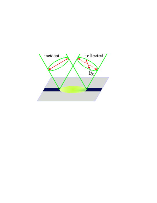
Figure 1: Schematic plot of the experimental configuration: a quantum wire (dark stripe) is illuminated by a linearly polarized beam and Kerr rotation angle of its polarization plane $\theta_{K}$ is measured. Polarizations of the beams are marked by double-headed arrows. Dashed arrow corresponds to the polarization of the reflected beam in the absence of the Kerr effect.

The spin noise spectroscopy, reviewed in Ref. Mueller et al. (2010), is based on the optical monitoring of the spin fluctuations Aleksandrov and Zapasskii (1981) in Faraday, Kerr or ellipticity signals measured with a weak linearly polarized probe beam incident on a single wire or a wire array sample, see Fig. 1. It can be shown similarly to Refs. Kos et al. (2010); Mueller et al. (2010); zhu07 that for the probe tuned to the fundamental absorption edge, the Kerr rotation angle $\theta_{K}\propto s_{z}$ ppwires , hence its autocorrelation function is directly related to the spin noise: $\langle\theta_{K}(t)\theta_{K}(t^{\prime})\rangle\propto\langle s_{z}(t)s_{z}(t^{\prime})\rangle$, where $s_{z}(t)$ is the density of the $z-$component of the total electron spin. As a result, this optical technique measures long-range correlations of equilibrium spin fluctuations occurring in the illuminated spot.

We consider a single channel quantum wire extended along the $x-$axis and represent the SO Hamiltonian as:

$$\mathcal{H}_{SO}=\frac{1}{2}[\alpha(x)k_{x}+k_{x}\alpha(x)]\sigma_{\lambda}.$$ (1)

Here $k_{x}=-\mathrm{i}\partial/\partial x$ is the electron wave vector component along the wire axis, $\alpha(x)$ is the coordinate-dependent SO coupling strength. In Eq. (1) we assumed that the spin quantization axis, $\lambda$, is fixed, and $\sigma_{\lambda}$ is the component of spin operator along this axis. The specific form of the SO Hamiltonian Eq. (1) implies that the effective field acting on electron spin points either parallel or antiparallel to the axis $\lambda$. This is obvious for a constant $\alpha(x)$  Nishimura et al. (1999); Governale and Zülicke (2002); de Andrada e Silva and La Rocca (2003); Entin and Magarill (2004); Glazov and Ivchenko (2004), and holds true provided that the microscopic symmetry of the fluctuations forming the SO coupling randomness is the same as overall symmetry of the system.

The SO coupling is assumed to be the sum of the coordinate-independent contribution, $\alpha_{0}$, and the Gaussian random function with zero average, $\alpha_{\rm r}(x)$ such as $\alpha(x)=\alpha_{0}+\alpha_{\rm r}(x)$ with the correlation function  Glazov et al. (2010):

$$\langle\alpha_{\rm r}(x)\alpha_{\rm r}(x^{\prime})\rangle=\langle\alpha_{\rm r}^{2}\rangle F_{\rm corr}(x-x^{\prime}),$$ (2)

where $\langle\alpha_{\rm r}^{2}\rangle$ is the mean square of SO coupling fluctuations and the range function $F_{\rm corr}(x-x^{\prime})$. We introduce also the typical correlation length of the SO coupling

$$l_{d}=\int_{0}^{\infty}F_{\rm corr}(x)\mathrm{d}x,$$ (3)

characterizing the size of the correlated domain of the random SO coupling. Details of the models of random SO coupling can be found in Ref.Glazov et al. (2010).

We begin with the semiclassical regime, where SO coupling disorder is smooth on the scale of electron wavelength, $l_{d}\gg\lambda_{\rm F}$, where the wavelength of the Fermi level electrons $\lambda_{\rm F}=2\pi/k_{\rm F}$, with $k_{\rm F}$ being the Fermi wave vector for the degenerate electron gas. The Hamiltonian (1) implies that the spin rotation angle around the $\lambda$-axis during the motion from the point $x_{0}$ to $x_{1}$ is

$$\theta(x_{1},x_{0})=\frac{2m}{\hbar^{2}}\int_{x_{0}}^{x_{1}}\alpha(x^{\prime})\mathrm{d}x^{\prime},$$ (4)

where $m$ is the electron effective mass. Eq. (4) shows that the angle is solely determined by electron initial and final positions and does not depend on the history of the motion between these points. This result, being well established for the systems with regular SO coupling Levitov and Rashba (2003); Entin and Magarill (2004); Tokatly and Sherman (2010, 2010); Slipko, Savran and Pershin (2011) holds also for the nanowires with the SO coupling disorder. As it follows from Eq. (1) the spin precession rate is proportional to the electron velocity and given coordinate-dependent function. Hence, it does not matter whether the electron starting from the point $x_{0}$ reached the point $x_{1}$ ballistically or diffusively: all contributions to spin precession of the closed paths, where electron passes the same configuration of $\alpha(x)$ in the opposite directions, cancel each other.

The temporal evolution of electron spin is directly related the electron motion along the wire. We consider here spin projections at given $z$ axis, perpendicular to the spin quantization axis $\lambda$. Time dependence of electron spin $z$ component averaged over its random spatial motion and over the random precession caused by the field $\alpha(x)$ can be most conveniently characterized by the correlator $\langle s_{z}(t)s_{z}(0)\rangle=\langle s_{z}^{2}(0)\rangle\mathcal{C}_{ss}(t)$ with the normalized correlation function:

$$\mathcal{C}_{ss}(t)=\int_{-\infty}^{\infty}\mathrm{d}x\ p(x,t)\langle\cos{[\theta(x,0)]}\rangle,$$ (5)

where $p(x,t)$ is the probability that electron travels distance $x$ during the time $t$. Note, that $\mathcal{C}_{ss}(t)$ can be understood as disorder-averaged electron spin $z$ component found with the initial condition $s_{z}(0)=1$. It results from the linearity of the spin dynamics equations: the correlators $\langle s_{i}(t)s_{j}(0)\rangle$ satisfy exactly the same equations as average values $\langle s_{i}(t)\rangle$ ($i,j=x,y,z$). In derivation of Eq. (5) we assumed also that the scattering of electrons, which determines $p(x,t)$ is not correlated with the random SO field $\alpha_{\rm r}(x)$, hence, the averaging over the realizations of $\alpha_{\rm r}(x)$ denoted by the angular brackets and over the trajectories can be considered independently. This can occur in nanowires where random Rashba fields are induced by doping while the momentum scattering is due to the wire width fluctuations. If the same local disorder determines the electron scattering and random SO fields, in relatively clean systems the electron mean free path $l$ exceeds by far the disorder correlation length $l_{d}$ in Eq.(3). Hence, spatial scales of two random processes: $l$ for the electron backward scattering in the random potential and $l_{d}$ for the spin precession are strongly different. As a result, on the $l$-scale, the memory of the short-range correlations is lost, and Eq. (5) holds. Although Eq. (5) is presented for the smooth SO coupling disorder, where the electron motion is semiclassical, $l_{d}/\lambda_{\mathrm{F}}\gg 1$, a general Green’s function approach confirms it for arbitrary $l_{d}/\lambda_{\mathrm{F}}$ values.

Our next step is to perform averaging of $\cos{[\theta(x,0)]}$ in Eq. (5) over the random realizations of the $\alpha(x)$-field. For this purpose we recast

$$\cos{[\theta(x,0)]}=\mathop{\rm Re}{\left\{\exp{\left(\mathrm{i}\frac{2m\alpha_{0}}{\hbar^{2}}x\right)}\exp{\left[\mathrm{i}\vartheta_{\rm r}(x)\right]}\right\}},$$ (6)

where

$$\vartheta_{\rm r}(x)=2m/\hbar^{2}\int_{0}^{x}\alpha_{\rm r}(x^{\prime})\mathrm{d}x^{\prime}$$ (7)

is the contribution of the random SO coupling into the spin rotation angle. We expand last exponent in series in $\vartheta_{\rm r}$ assuming the Gaussian SO coupling disorder. In the averaging, odd powers of spin rotation angle vanish, $\langle\theta_{\rm r}^{2n+1}(x)\rangle=0$, for integer $n$ and even powers can be expressed solely with $\langle\theta_{\rm r}^{2}(x)\rangle$ as

$$\langle\theta_{\rm r}^{2n}(x)\rangle=\left\langle\left[\frac{2m}{\hbar^{2}}\int_{0}^{x}\alpha_{\rm r}(x^{\prime})\mathrm{d}x^{\prime}\right]^{2n}\right\rangle=(2n-1)!!\langle\theta_{\rm r}^{2}(x)\rangle^{n}.$$ (8)

Direct calculation shows that the mean square $\langle\theta_{\rm r}^{2}(x)\rangle$ caused by the random SO interaction is given by

$$\langle\theta_{\rm r}^{2}(x)\rangle=2\left(\frac{2m}{\hbar^{2}}\right)^{2}\langle\alpha_{\rm r}^{2}\rangle\int_{0}^{x}\mathrm{d}x^{\prime}\int_{0}^{x^{\prime}}\mathrm{d}yF_{\rm corr}(y).$$ (9)

Finally, Eq. (5) reduces to

$$\mathcal{C}_{ss}(t)=\int_{-\infty}^{\infty}\mathrm{d}x\ p(x,t)\cos{\left(\frac{2m\alpha_{0}}{\hbar^{2}}x\right)}\exp{\left[-\langle\theta_{\rm r}^{2}(x)\rangle/2\right]}.$$ (10)

When $\langle\theta_{\rm r}^{2}(x)\rangle$ becomes considerably larger than one, spins are completely dephased. Equation (10) is our central result: it relates temporal average spin dynamics with electron motion along the wire. Distribution function of electron displacements, $p(x,t)$, presented for different regimes of electron motion below, enables us to calculate spin evolution by Eq. (10). The spin noise power spectrum is given by the transform of $\mathcal{C}_{ss}(t)$ Kos et al. (2010):

$$\left\langle s_{z}^{2}\right\rangle_{\omega}=2\int_{0}^{\infty}\mathcal{C}_{ss}(t)\cos\left(\omega t\right){\rm d}t.$$ (11)

To get a better insight into the problem, we begin with the key limits footnote . First, for the ballistic electron dynamics $p(x,t)=\delta(x-v_{\rm F}t)$, where $v_{\rm F}=\hbar k_{\rm F}/m$ is the Fermi velocity. The ballistic motion is realized on the temporal scale $t\ll\tau=l/v_{\rm F}$ with $\tau$ being the momentum relaxation time. We are interested in the spin dynamics on the time scale $t\gg\tau_{d}=l_{d}/v_{\rm F}$, where $\tau_{d}$ is the time during which electron passes the correlated interval of the SO coupling fluctuations. Using Eq. (10) we obtain damped oscillations of the spin $z$-component:

$$\mathcal{C}_{ss}(t)\approx\cos{\left(\Omega_{0}t\right)}\exp{\left(-t/\tau_{s,{\rm r}}\right)},$$ (12)

with the frequency $\Omega_{0}={2m\alpha_{0}v_{\rm F}}/{\hbar^{2}}$ determined by the averaged SO coupling and the decay time caused by the SO coupling fluctuations

$$\frac{1}{\tau_{s,{\rm r}}}=\left(\frac{2mv_{\rm F}}{\hbar^{2}}\right)^{2}\langle\alpha_{\rm r}^{2}\rangle\tau_{d}.$$ (13)

Equation (13) for the spin relaxation time $\tau_{s,{\rm r}}$ is a result of random spin precession Glazov et al. (2010). Spin noise power spectrum calculated using Eqs. (11) and (12) reads:

$$\left\langle s_{z}^{2}\right\rangle_{\omega}=2\tau_{s,\rm r}\mathop{\rm Re}\frac{1-\mathrm{i}\omega\tau_{s,\rm r}}{\Omega_{0}^{2}\tau_{s,\rm r}^{2}+(1-\mathrm{i}\omega\tau_{s,\rm r})^{2}}$$ (14)

with the result presented in Fig. 2.

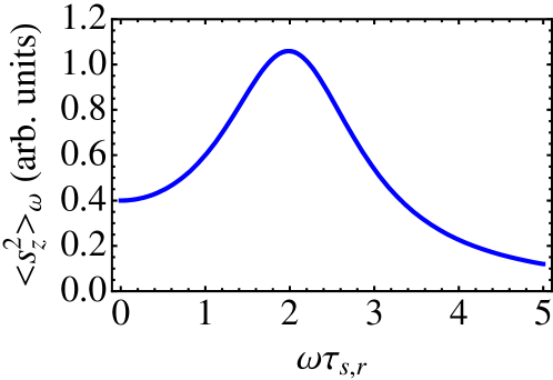
Figure 2: Spin noise power spectrum, $\langle s_{z}^{2}\rangle_{\omega}$, for ballistic propagation, $\Omega_{0}\tau_{s,\rm r}=2$. Due the exponential decay in Eq.(12) it is finite at $\omega=0$ with the width determined by the spin relaxation time $\tau_{s,\rm r}$. The spectrum peaks at the frequency $\Omega_{0}$ since average electron spin rotates in the SO field at the rate $\Omega_{0}$ and asymptotically decays as $\omega^{-2}$ in accordance with the fluctuation-dissipation theorem.

This ballistic regime of spin dynamics, however, can be realized only in very clean systems, where $\Omega_{0}\tau\gg 1$. Otherwise, electron spin evolution occurs at the time scale, where electron moves diffusively (Fig.3, upper panel), i.e.

$$p(x,t)=\frac{1}{2\sqrt{\pi Dt}}e^{-{x^{2}}/{4Dt}},$$ (15)

where $D=v_{\rm F}^{2}\tau$ is the diffusion coefficient. In the absence of the SO coupling fluctuations and provided that $\Omega_{0}\tau\ll 1$ exponential spin relaxation is due to the Dyakonov-Perel’ mechanism Nishimura et al. (1999); Glazov and Ivchenko (2004) with the relaxation time $\tau_{s,\rm DP}=1/(\Omega_{0}^{2}\tau)$. The spin noise spectrum has a Lorentzian form $\langle s_{z}^{2}\rangle_{\omega}=2\tau_{s,\rm DP}/(1+\omega^{2}\tau_{s,\rm DP}^{2})$ with the width determined by the relaxation time.

New physical features arise when the SO coupling fluctuations dominate over the regular contribution. From now on we put $\alpha_{0}=0$ and consider the system where SO coupling is purely random and concentrate on the long-time ($t\gg\tau_{d},\tau,\tau_{s,\rm r}$) dynamics. At these times, the system in Eq. (10) is characterized by two length parameters. One parameter is the diffusion length $\sqrt{Dt}$ in Eq. (15), the other one

$$L_{s}=\int_{0}^{\infty}\mathrm{d}x\exp{\left[-\langle\theta_{\rm r}^{2}(x)\rangle/2\right]},$$ (16)

characterizes spin randomization. At sufficiently long times, when $\sqrt{Dt}\gg L_{s}$, one can take $p(0,t)$ instead of $p(x,t)$ and immediately obtain from Eq. (10) that the relaxation is algebraic rather than exponential:

$$\mathcal{C}_{ss}(t)\approx p(0,t)\int_{-\infty}^{\infty}\mathrm{d}x\exp{\left[-\langle\theta_{\rm r}^{2}(x)\rangle/2\right]}=\frac{L_{s}}{\sqrt{\pi Dt}}.$$ (17)

Equation (17) predicts extremely long spin decoherence described by the inverse square root law: $\langle s_{z}(t)\rangle\propto 1/\sqrt{t}$. This surprising result has a transparent physical interpretation (see Fig. 3): Indeed, if an electron is displaced from its initial position by a sufficiently large distance, $x\gtrsim L_{s}$, its spin rotation angle becomes so large, that it does not contribute to the total spin polarization owing to $\exp{\left[-\langle\theta_{\rm r}^{2}(x)\rangle/2\right]}$ in Eq. (10). As a result, the spin polarization is supported by the electrons located in the vicinity of their initial positions, mainly due to the return after multiple scatterings by the random potential. The fraction of such electrons, in agreement with the diffusion distribution, decays as $p(0,t)\propto 1/\sqrt{t}$ resulting in the same behavior in the spin polarization. It is interesting to mention that this qualitative argument does not work for the constant SO coupling despite spin of electron is restored upon the return to the origin also here. The reason is that due the oscillations of the spin on the spatial scale of the order of $\hbar^{2}/m\alpha_{0}$ (see Fig. 3, lower panel) in Eq.(10), the diffusive return of electrons to the origin is insufficient for formation of the algebraic relaxation tail.

Another realization of the $1/\sqrt{t}$ spin decay can be achieved for the very strong random SO couping where the spin relaxation occurs within one nanosize domain of the SO coupling, that is at the electron displacement much less than $l_{d}$. In this case, spin relaxation rate is due to the Dyakonov-Perel’ mechanism and is determined by the local value of $\alpha(x)$ inside the domain. Spins of electrons located in the intervals with large $\alpha(x)$ will relax fast, while spins of those experiencing weak $\alpha(x)$ will relax slow.

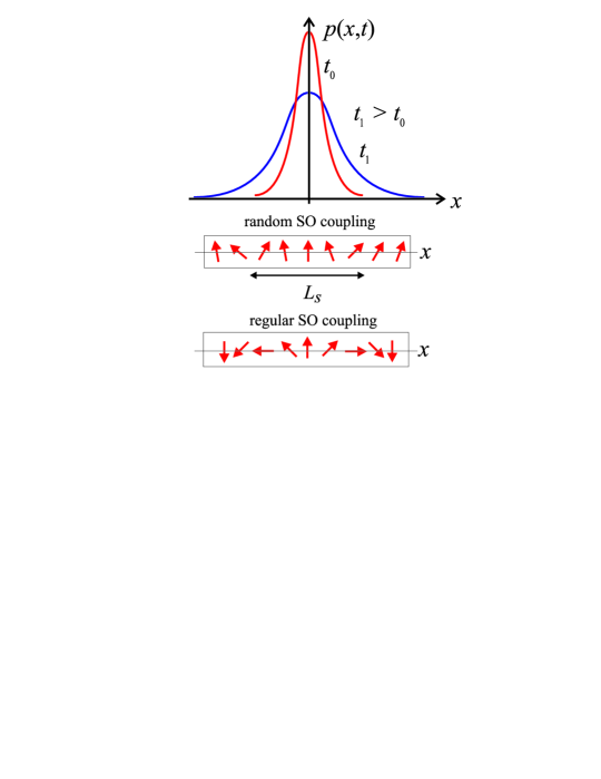
Figure 3: Upper panel: Schematic illustration of the displacements distribution $p(x,t)$ for two different time moments: $t_{0}<t_{1}$. Lower panels: The quantum wire and spins of diffusing electron for the random and regular SO couplings, respectively. For the random SO coupling, if the electron is within the $L_{s}$ distance from its initial point [see Eq. (17)] its spin is preserved, when it leaves this interval, the spin dephases.

Slow non-exponential spin relaxation, described by Eq. (17) manifests itself in the low frequency spin noise spectrum. From Eq. (11) it follows: $\left\langle s_{z}^{2}\right\rangle_{\omega}\propto{1}/{\sqrt{\omega}}$, i.e the spin noise diverges at $\omega\to 0$. Such a non-trivial behavior is inherent to the quantum wires with random SO coupling, where spin restores upon return to the origin: in multichannel wires for sufficiently fast interchannel scattering footnote1 and in two-dimensional systems spin relaxation is exponential Glazov et al. (2010) and $\left\langle s_{z}^{2}\right\rangle_{\omega=0}$ is finite.

To conclude, we studied theoretically spin noise in semiconductor nanowire for different regimes of the electron propagation. We demonstrated that if the spin relaxation is determined by the randomness in the SO coupling, spin relaxation becomes algebraic being closely related to the high probability for electron to stay close to its initial position as a result of a multiple scatterings in the random potential. This behavior can appear in at least two possible regimes: (i) when the electron motion is diffusive and (ii) when the spin relaxation occurs on a small spatial scale of the order of 10 nm. In any of these cases, the spin noise power spectrum shows colored ${1}/{\sqrt{\omega}}$ noise. In addition, this observation shows that low-frequency optical spin noise spectroscopy is an excellent tool for studying spin phenomena in semiconductor nanowires and characterization of random potential and SO coupling there.

Acknowledgements MMG is grateful to RFBR and “Dynasty” Foundation—ICFPM for financial support. This work of EYS was supported by the University of Basque Country UPV/EHU grant GIU07/40, MCI of Spain grant FIS2009-12773-C02-01, and ”Grupos Consolidados UPV/EHU del Gobierno Vasco” grant IT-472-10.

Supplementary Material for “Theory of Spin Noise in Nanowires”

I SI. Spin noise at arbitrary frequencies

Here we determine the spin noise spectrum for arbitrary frequencies $\omega$. We employ the kinetic equation for electron distribution function $f(x,v_{x},t)$ dependent on the position, velocity $v_{x}$, and time. The equation has the form:

$$\frac{\partial f}{\partial t}+v_{x}\frac{\partial f}{\partial x}+\frac{f-\bar{f}}{\tau}=0,$$

where $f(x,v_{x},t)$ satisfies the initial condition $f(x,v_{x},0)=\delta(x)[\delta_{v,v_{\rm F}}+\delta_{v,-v_{\rm F}}]/2$ meaning that at $t=0$ it is built at $x=0$ with the equal fractions of electrons with velocities $v_{x}=\pm v_{\rm F}$. As a result, the carriers can be separated into the right movers, $v_{x}=v_{\rm F}$, and left movers, $v_{x}=-v_{\rm F}$ with function $\bar{f}=[f(x,v_{\rm F},t)-f(x,-v_{\rm F},t)]/2$ being the anisotropic part of the distribution. The distribution of electron displacements is given by $p(x,t)=f(x,v_{\rm F},t)+f(x,-v_{\rm F},t)$. It can be shown that the spatial Fourier transform and $\cos(\omega t)$ transform of this distribution, $\tilde{p}(k,\omega)$ has the form

$$\tilde{p}(k,\omega)=2\mathop{\rm Re}\frac{\tau(1-\mathrm{i}\omega\tau)}{(kl)^{2}-\mathrm{i}\omega\tau(1-\mathrm{i}\omega\tau)}.$$

In accordance with Eq. (11) in the main text the spin noise spectrum can be presented as

$$\left\langle s_{z}^{2}\right\rangle_{\omega}=\int_{-\infty}^{\infty}\frac{\mathrm{d}k}{2\pi}\ \tilde{p}(k,\omega)\mathcal{T}(k),$$

where

$$\mathcal{T}(k)=\int_{-\infty}^{\infty}\exp{\left[\mathrm{i}kx-\langle\theta_{\rm r}^{2}(x)\rangle/2\right]}\mathrm{d}x.$$

Analytical result can be obtained in the regime where spin rotation angles within each correlated domain of the SO coupling are small, that is $\Omega_{\rm r}\tau_{d}\equiv 2m\sqrt{\langle\alpha_{r}^{2}\rangle}l_{d}/\hbar\ll 1$ with $\Omega_{\rm r}\equiv 2\sqrt{\langle\alpha_{r}^{2}\rangle}k_{x}/\hbar$. Here the spin dynamics occurs on the spatial scale $x\gg l_{d}$, mean squares of spin rotation angles are proportional to electron displacement $\langle\theta_{\rm r}^{2}(x)\rangle\approx 2(\Omega_{\rm r}\tau_{d})^{2}|x|/l_{d}$ being valid for $x\gg l_{d}$ or at $t\gg\tau_{d}$, and function $\mathcal{T}(k)$ takes the form:

$$\mathcal{T}(k)=\frac{2l_{d}(\Omega_{r}\tau_{d})^{2}}{(\Omega_{r}\tau_{d})^{4}+(kl_{d})^{2}}.$$

After lengthy transformations we obtain

$$\langle s_{z}^{2}\rangle_{\omega}=2\mathop{\rm Re}\frac{\tau_{d}}{(\Omega_{r}\tau_{d})^{2}\sqrt{{\mathrm{i}\omega\tau}/{(\mathrm{i}\omega\tau-1)}}-\mathrm{i}\omega\tau_{d}}.$$

It can be seen from Eq. (S6) that at low frequencies, $\omega\ll\tau_{d}^{-1},\tau^{-1}$, spin noise spectrum has the form:

$$\left\langle s_{z}^{2}\right\rangle_{\omega}=\frac{\sqrt{2}\tau_{s,\rm r}}{\sqrt{\omega\tau}},$$

in agreement with the analysis above. For high frequencies $\omega\tau\gg 1$, $\left\langle s_{z}^{2}\right\rangle_{\omega}$ is given by $2/(\omega^{2}\tau_{s,\rm r})$ since at $\tau_{d}\ll t\ll\tau$ the electron motion is ballistic, and spin dephasing is caused by the random fluctuations of the spin-orbit coupling, cf. Eq. (12) of the main text. The entire frequency dependence of $\left\langle s_{z}^{2}\right\rangle_{\omega}$ is plotted in Fig. 4.

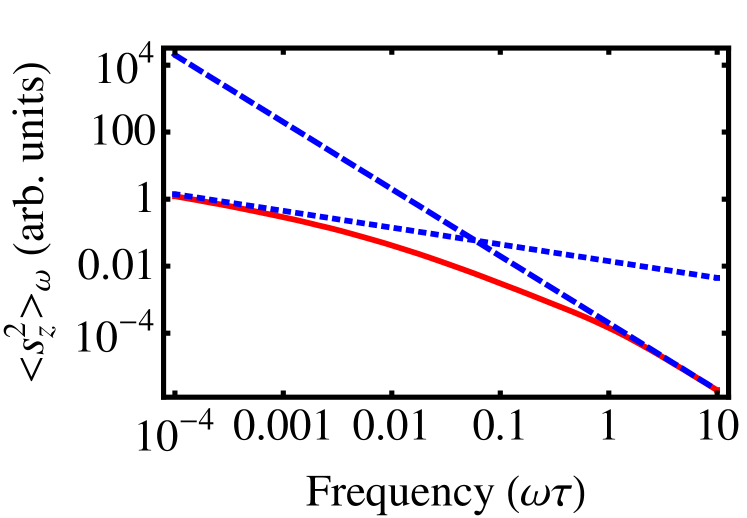
Figure 4: Spin noise power spectrum for diffusive electron propagation, $\Omega_{0}\equiv 0$, $\Omega_{\rm r}\tau_{d}=0.01$, $\tau_{d}/\tau=0.1$. Solid line shows exact result, calculated according to Eq. (S6). Dotted (with the slope -1/2) and dashed (with the slope -2) lines show the low-frequency and high-frequency asymptotic, respectively.

II SII. Spin dynamics and noise in multichannel wires with random spin-orbit coupling

The spin evolution in multichannel structures depends on the additional set of parameters, $\{\tau_{i,j}\}$ being the scattering times between the channels $i$ and $j$, as well as on the details of spin dynamics in every channel. For qualitative analysis (a general case requires a separate treatment) we consider a structure with two conducting channels, where (i) spin-orbit coupling disorder in different channels is not correlated and (ii) in each channel $\Omega_{\rm r}^{[c]}\tau_{d}\ll 1$ (superscripts denote channels), i.e. spin rotation angles in correlated domains of the spin-orbit coupling are always small. Here we can characterize the interchannel scattering by a single time $\tau_{c}$ and focus on the most interesting case with no regular contribution to the spin-orbit field: $\alpha_{0}\equiv 0$.

In the limit of very rare interchannel scattering events (the condition is given below) the channels are independent. Hence, the general results expressed by Eqs. (10), (11) of the main text and by Eq. (S6) as well as asymptotic Eqs. (S7) and (17) of the main text hold. Although in these equations one has to average over the realizations of $\alpha_{\rm r}^{[c]}(x)$ in different channels, the low-frequency spin noise power spectrum remains $1/\sqrt{\omega}$, the same as in a single channel wire.

Now we turn to the efficient interchannel scattering with short $\tau_{c}$. If $\tau_{c}\ll\tau_{d}$ electron quits given channel faster than it quits the correlated domain. Spin rotations between interchannel scattering events are uncorrelated and, due to this randomness, spin dynamics is exponential:

$$\langle s_{z}(t)s_{z}(0)\rangle\propto\exp{\left(-{\Gamma_{c}{t}}\right)},$$

where the relaxation rate $\Gamma_{c}$ is of the order of $\left[\max{\left\{\Omega_{\rm r}^{[1]},\Omega_{\rm r}^{[2]}\right\}}\right]^{2}\tau_{c}.$ Similar exponential decay of the spin correlator remains for $\tau_{d}\ll\tau_{c}\ll\tau$. Here, the mean square of the spin rotation angle between interchannel scatterings can be estimated as $\langle(\delta\Phi)^{2}\rangle=\langle\theta_{\rm r}^{2}(v^{[c]}\tau_{c})\rangle\propto\tau_{c}$, with $v^{[c]}$ being the characteristic velocity in the channel. Spin relaxation is governed by the Dyakonov-Perel’-like mechanism, with the rate

$$\Gamma\propto\langle(\delta\Phi)^{2}\rangle/\tau_{c}\sim\tau_{s,\rm r}^{-1},$$

which is $\tau_{c}$-independent for exactly the same reason as the spin relaxation rate due to the random spin-orbit [Eq.(13) in the main text] does not explicitly depend on the electron free path.

Most interesting physics appears for a very weak interchannel scattering, $\tau_{c}\gg\tau,\tau_{d}$. In this case, electron moves diffusively in a given channel before the interchannel scattering occurs. As we have shown above, the $1/\sqrt{t}$ tail in the spin polarization (and corresponding $1/\sqrt{\omega}$ spin noise) results from the carriers dwelling around the initial point of their trajectories. Since the tail is formed at long times $\sqrt{Dt}\gg L_{s}$, see Eq. (16) of the main text, it is supported by electrons which moved many times back and forth in the random potential. If the interchannel scattering is probable, electron may return to the initial point via other channels, where its spin rotation is not correlated with that in the initial one. Therefore, in general $1/\sqrt{t}$ tail is destroyed and the usual exponential spin relaxation takes place. However, if $\tau_{c}$ is long enough to assure that the typical electron displacement during the diffusion between interchannel scatterings $L_{c}=\sqrt{D\tau_{c}}\gg L_{s}$, there is a time interval ${L_{s}^{2}}/{D}\ll t\ll\tau_{c}$ and the corresponding frequency range, where the spin dynamics and the noise are algebraic:

$$\langle s_{z}(t)s_{z}(0)\rangle\propto\frac{1}{\sqrt{t}},\ \langle s_{z}^{2}\rangle_{\omega}\propto\frac{1}{\sqrt{\omega}}.$$

In the regimes of a highly efficient interchannel scattering, with the spin relaxation described by Eqs.(S8) or (S9), the probability of spin components restoration upon return to the initial position is strongly suppressed, and, as a result, spin noise power spectrum at low frequency decreases and becomes finite.

For completeness, we mention that if the random spin-orbit coupling does not depend on the channel, that is $\alpha_{\rm r}^{[1]}(x)=\alpha_{\rm r}^{[2]}(x)$, spin precession angle between any points $x_{1}$ and $x_{2}$ is insensitive to the interchannel scattering, and our analysis in the main text holds exactly the same.

References

- Zutic et al. (2004) I. Zutic, J. Fabian, and S. DasSarma, Rev. Mod. Phys. 76, 323 (2004).
- Wu et al. (2010) M. Wu, J. Jiang, and M. Weng, Phys. Reports 493, 61 (2010).
- (3) E.L. Ivchenko, Sov. Phys. Semicond. 7, 998 (1974).
- Mueller et al. (2010) G. M. Müller, M. Oestreich, M. Römer, and J. Hübner, Physica E 43, 569 (2010).
- Müller et al. (2008) G. M. Müller, M. Römer, D. Schuh, W. Wegscheider, J. Hübner, and M. Oestreich, Phys. Rev. Lett. 101, 206601 (2008).
- Crooker et al. (2010) S. A. Crooker, J. Brandt, C. Sandfort, A. Greilich, D. R. Yakovlev, D. Reuter, A. D. Wieck, and M. Bayer, Phys. Rev. Lett. 104, 036601 (2010).
- Braun and König (2007) M. Braun and J. König, Phys. Rev. B 75, 085310 (2007).
- Starosielec and Hägele (2008) S. Starosielec and D. Hägele, Appl. Phys. Lett. 93, 051116 (2008).
- Kos et al. (2010) S. S. Kos, A. V. Balatsky, P. B. Littlewood, and D. L. Smith, Phys. Rev. B 81, 064407 (2010).
- Kiselev and Kim (2000) A. A. Kiselev and K. W. Kim, Phys. Rev. B 61, 13115 (2000).
- Pramanik et al. (2003) S. Pramanik, S. Bandyopadhyay, and M. Cahay, Phys. Rev. B 68, 075313 (2003).
- Holleitner et al. (2006) A. W. Holleitner, V. Sih, R. C. Myers, A. C. Gossard, and D. D. Awschalom, Phys. Rev. Lett. 97, 036805 (2006).
- Quay et al. (2010) C. H. L. Quay, T. L. Hughes, J. A. Sulpizio, L. N. Pfeiffer, K. W. Baldwin, K. W. West, D. Goldhaber-Gordon, and R. de Picciotto, Nat. Phys 6, 336 (2010).
- Pershin, Nesteroff and Privman (2004) Y. V. Pershin, J. A. Nesteroff, and V. Privman, Phys. Rev. B 69, 121306 (2004).
- Nadj-Perge et al. (2010) S. Nadj-Perge, S. Frolov, E. Bakkers, and L. Kouwenhoven, Preprint arXiv:1011.0064 (2010).
- Bringer and Schäpers (2011) A. Bringer and T. Schäpers, Phys. Rev. B 83, 115305 (2011).
- Nishimura et al. (1999) T. Nishimura, X.-L. Wang, M. Ogura, A. Tackeuchi, and O. Wada, Japan. Journ. of Appl. Phys. 38, L941 (1999).
- Governale and Zülicke (2002) M. Governale and U. Zülicke, Phys. Rev. B 66, 073311 (2002).
- de Andrada e Silva and La Rocca (2003) E. A. de Andrada e Silva and G. C. La Rocca, Phys. Rev. B 67, 165318 (2003).
- Entin and Magarill (2004) M. V. Entin and L. I. Magarill, Europhys. Lett. 68, 853 (2004).
- Glazov and Ivchenko (2004) M. M. Glazov and E. L. Ivchenko, JETP 99, 1279 (2004).
- Averkiev and Golub (1999) N. S. Averkiev and L. E. Golub, Phys. Rev. B 60, 15582 (1999).
- Gryncharova and Perel’ (1976) E. Gryncharova and V.I. Perel’, Sov. Phys. Semicond. 10, 2272 (1976).
- Sherman (2003a) E. Ya. Sherman, Phys. Rev. B 67, 161303 (2003a).
- Sherman (2003b) E.Ya. Sherman, Appl. Phys. Lett. 82, 209 (2003b).
- V. K. Dugaev, E. Ya. Sherman, V. I. Ivanov, and J. Barnas (2009) V.K. Dugaev, E.Ya. Sherman, V.I. Ivanov, and J. Barnaś, Phys. Rev. B 80, 081301 (2009).
- Golub and Ivchenko (2004) L. Golub and E.L. Ivchenko, Phys. Rev. B 69, 115333 (2004).
- Glazov and Sherman (2005) M.M. Glazov and E.Ya. Sherman, Phys. Rev. B 71, 241312 (2005).
- Glazov et al. (2010) M.M. Glazov, E.Ya. Sherman, and V.K. Dugaev, Physica E 42, 2157 (2010).
- (30) A. Ström, H. Johannesson, and G. I. Japaridze, Phys. Rev. Lett. 104, 256804 (2010).
- Dutta and Horn (1981) P. Dutta and P. M. Horn, Rev. Mod. Phys. 60, 53 (1981).
- Weissman (1988) M. B. Weissman, Rev. Mod. Phys. 60, 537 (1988).
- Levinshtein (1997) M.E. Levinshtein, Physica Scripta T69, 79 (1997).
- Aleksandrov and Zapasskii (1981) E. Aleksandrov and V. Zapasskii, JETP 54, 64 (1981).
- (35) E. A. Zhukov et al., Phys. Rev. B 76, 205310 (2007).
- Levitov and Rashba (2003) L. S. Levitov and E. I. Rashba, Phys. Rev. B 67, 115324 (2003).
- Tokatly and Sherman (2010) I.V. Tokatly and E.Ya. Sherman, Annals of Physics 325, 1104 (2010).
- Tokatly and Sherman (2010) I.V. Tokatly and E.Ya. Sherman, Phys. Rev. B 82, 161305 (2010).
- Slipko, Savran and Pershin (2011) V.A. Slipko, I. Savran, and Y. V. Pershin, Phys. Rev. B 83, 193302 (2011).
- (40) The Kerr rotation can be calculated using the methods of I. A. Yugova et al., Phys. Rev. B 80, 104436 (2009) and E. L. Ivchenko, A. V. Kavokin, Sov. Phys. Solid State 34, 1815 (1992).
- (41) The general case is treated in the Supplementary Material.
- (42) Various regimes of spin dynamics in multichannel nanowires are briefly discussed in the Supplementary Material.