Accuracy of the post-Newtonian approximation. II. Optimal asymptotic expansion of the energy flux for quasicircular, extreme mass-ratio inspirals into a Kerr black hole.

Abstract

We study the effect of black hole spin on the accuracy of the post-Newtonian approximation. We focus on the gravitational energy flux for the quasicircular, equatorial, extreme mass-ratio inspiral of a compact object into a Kerr black hole of mass $M$ and spin $J$. For a given dimensionless spin $a\equiv J/M^{2}$ (in geometrical units $G=c=1$), the energy flux depends only on the orbital velocity $v$ or (equivalently) on the Boyer-Lindquist orbital radius $r$. We investigate the formal region of validity of the Taylor post-Newtonian expansion of the energy flux (which is known up to order $v^{8}$ beyond the quadrupole formula), generalizing previous work by two of us. The error function used to determine the region of validity of the post-Newtonian expansion can have two qualitatively different kinds of behavior, and we deal with these two cases separately. We find that, at any fixed post-Newtonian order, the edge of the region of validity (as measured by $v/v_{{\mbox{\tiny ISCO}}}$, where $v_{{\mbox{\tiny ISCO}}}$ is the orbital velocity at the innermost stable circular orbit) is only weakly dependent on $a$. Unlike in the nonspinning case, the lack of sufficiently high order terms does not allow us to determine if there is a convergent to divergent transition at order $v^{6}$. Independently of $a$, the inclusion of angular multipoles up to and including $\ell=5$ in the numerical flux is necessary to achieve the level of accuracy of the best-known ($N=8$) PN expansion of the energy flux.

I Introduction

Binaries of compact objects, such as black holes (BHs) and/or neutron stars, are one of the main targets for gravitational-wave (GW) observations. When the binary members are widely separated, their slow inspiral can be well-described by the post-Newtonian (PN) approximation, a perturbative asymptotic expansion of the “true” solution of the Einstein equations. The small expansion parameter in the PN approximation is $v/c$, where $v$ is the orbital velocity of the binary and $c$ is the speed of light. Asymptotic expansions, however, must be used with care, as the inclusion of higher-order terms does not necessarily lead to an increase in accuracy. Therefore one would like to determine the optimal order of expansion and the formal region of validity of the PN asymptotic series Bender:1978 ; Yunes:2008tw , i.e. the order and region inside which the addition of higher order terms increases the accuracy of the approximation in a convergent fashion.

In a previous paper (Yunes:2008tw , henceforth Paper I), two of us investigated the accuracy of the PN approximation for quasicircular, nonspinning (Schwarzschild), extreme mass-ratio inspirals (EMRIs). By comparing the PN expansion of the energy flux to numerical calculations in the perturbative Teukolsky formalism, we concluded that (i) the region of validity of the PN expansion is largest at relative 3PN order – i.e., order $(v/c)^{6}$ (throughout this paper, a term of ${\cal{O}}(v^{2N})$ is said to be of $N$PN order); and (ii) the inclusion of higher multipoles in numerical calculations is necessary to improve the agreement with PN expansions at large orbital velocities. The fact that the region of validity is largest at 3PN could be a hint that the series actually diverges beyond 3PN order, at least in the extreme mass-ratio limit.

This paper extends our study to EMRIs for which the more massive component is a rotating (Kerr) BH. The present analysis focuses on the effect of the BH spin on the accuracy of the PN expansion. We generalize the methods presented in Paper I to take into account certain pathological behaviors of the error function, used to determine the region of validity. This generalization may also be applicable to comparable-mass systems.

A surprising result we find is that the edge of the region of validity (the maximum velocity beyond which higher-order terms in the series cannot be neglected), normalized to the velocity at the innermost stable circular orbit, is weakly dependent on the Kerr spin parameter $a$. In fact, this edge is roughly in the range $v/v_{{\mbox{\tiny ISCO}}}\in[0.3,0.6]$ for almost all PN orders, irrespective of $a$. This suggests, perhaps, that the ratio $v/v_{{\mbox{\tiny ISCO}}}$ is a better PN expansion parameter than $v/c$, when considering spinning BHs.

Another surprising result is related to the behavior of the edge of the region of validity as a function of PN order. In the nonspinning case, two of us found that beyond 3PN order, ${\cal{O}}(v^{6}/c^{6})$, this edge seemed to consistently decrease with PN order Yunes:2008tw . This was studied up to ${\cal{O}}(v^{11}/c^{11})$, the largest PN order known for the nonspinning case. In the spinning case, however, the series is known only up to ${\cal{O}}(v^{8}/c^{8})$, and we are thus unable to conclusively determine if the trend found in the nonspinning case persists. Higher-order calculations will be necessary to draw more definite conclusions.

Numerical (or in this case, perturbative) calculations of the energy flux rely on multipolar decompositions of the angular dependence of the radiation. By comparing the convergence of the multipolar decomposition to the convergence of the PN expansion of the energy flux, we find that for $v/c\sim 0.1$ the inclusion of multipoles up to and including $\ell=5$ seems necessary to achieve the level of accuracy of the best-known ($N=8$) PN expansion of the flux. These conclusions are also largely independent of the spin parameter $a$.

The rest of this paper is organized as follows. In Section II we present the energy flux radiated by quasicircular, equatorial Kerr EMRIs in the adiabatic approximation, as computed in PN theory Poisson:1995vs ; Tagoshi:1996gh ; Tanaka:1997dj and with accurate frequency-domain codes in BH perturbation theory 2009GWN…..2….3Y ; Yunes:2009ef ; Yunes:2010zj . In Section III we discuss the region of validity of the PN approximation in terms of the normalized orbital velocity $v/v_{{\mbox{\tiny ISCO}}}$ and of the normalized orbital radius $r/r_{{\mbox{\tiny ISCO}}}$, where ISCO stands for the innermost stable circular orbit. We consider both corotating and counterrotating orbits. In Section IV we study the number of multipolar components that must be included in the numerical flux in order to achieve sufficient accuracy. Finally, in Section V we present our conclusions. We follow the same notation as in Paper I. In particular, from now on we will use geometrical units ($G=c=1$).

II Energy flux for quasicircular, equatorial EMRIs in Kerr: numerical and PN results

In the PN approximation, the GW energy flux radiated to infinity by a test particle in a circular orbit and on the equatorial plane of a Kerr BH is given by Tagoshi:1996gh ; Tanaka:1997dj ; Poisson:1995vs

$$F^{(N)}=F_{\rm Newt}\left[\sum_{k=0}^{N}(a_{k}+b_{k}\,\ln v)\,v^{k}\right]\,.$$ (1)

This flux is known up to $N=8$ when including spins, and up to $N=11$ in the nonspinning case. The leading (Newtonian) contribution is

$$F_{\rm Newt}=\frac{32}{5}\frac{\mu^{2}}{M^{2}}v^{10}\,,$$ (2)

where $\mu$ and $M$ are the test particle mass and Kerr BH mass, respectively. As we are here interested in the accuracy of the PN approximation, we will ignore the flux of energy going into the horizon, which cannot always be neglected when building waveform templates.

The expansion coefficients $a_{k}$ and $b_{k}$ contain both spin-independent and spin-dependent terms, where the dimensionless spin parameter $a$ is related to the Kerr BH spin angular momentum via $J=aM^{2}$. These coefficients can be found in Eq. (G19) of Tagoshi:1996gh , so we do not list them explicitly. Note that logarithmic terms only appear at 3PN and 4PN (i.e., $b_{6}\neq 0$ and $b_{8}\neq 0$), and that the $(a_{k},b_{k})$ for $8<k\leq 11$ are known only in the spin-independent limit.

Throughout this paper $v$ is the orbital velocity, defined as $v\equiv(M\Omega)^{1/3}$ (where $\Omega$ is the small body’s orbital frequency), and related to the Boyer-Lindquist radius $r$ by

$$\frac{r}{M}=\frac{(1-av^{3})^{2/3}}{v^{2}}\,,$$ (3)

whose inverse is

$$v=\left[(r/M)^{3/2}+a\right]^{-1/3}\,.$$ (4)

At the ISCO we have Bardeen:1972fi

$$\frac{r_{{\mbox{\tiny ISCO}}}}{M} = 3+Z_{2}-\sqrt{(3-Z_{1})(3+Z_{1}+2Z_{2})}\,,$$ (5)

$$Z_{1} \equiv 1+(1-a^{2})^{1/3}\left[(1+a)^{1/3}+(1-a)^{1/3}\right]\,,$$

$$Z_{2} \equiv (3a^{2}+Z_{1}^{2})^{1/2}\,,$$ (6)

where $a>0$ ($a<0$) corresponds to corotating (counterrotating) orbits.

Using Eqs. (3) and (5), we also have

$$\frac{r}{r_{{\mbox{\tiny ISCO}}}}=\frac{(1-av^{3})^{2/3}}{v^{2}\left[3+Z_{2}\mp\sqrt{(3-Z_{1})(3+Z_{1}+2Z_{2})}\right]}\,.$$

The ISCO velocity can be found by replacing $r_{{\mbox{\tiny ISCO}}}$ in Eq. (5) into the velocity-radius relation (4). The velocity $v_{{\mbox{\tiny ISCO}}}$ and the radius $r_{{\mbox{\tiny ISCO}}}/M$ are displayed graphically in Fig. 1. Observe that, although $r_{{\mbox{\tiny ISCO}}}\to M$ as $a\to 1$, $v_{{\mbox{\tiny ISCO}}}$ is bounded by $2^{-1/3}\simeq 0.79$.

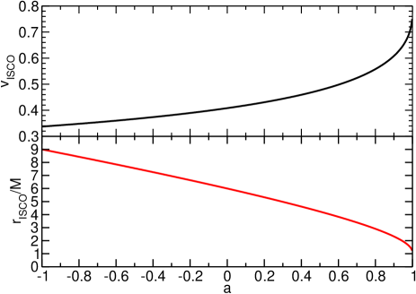
Figure 1: ISCO velocity ($v_{{\mbox{\tiny ISCO}}}$, top panel) and radius ($r_{{\mbox{\tiny ISCO}}}/M$, bottom panel) as a function of $a$. Here and elsewhere we use the convention that a negative spin parameter refers to counterrotating orbits.

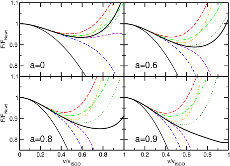
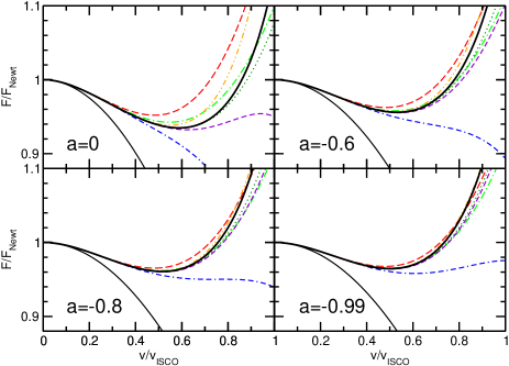
Figure 2: Gravitational energy flux (normalized to $F_{\rm Newt}$) as a function of the normalized orbital velocity, $v/v_{{\mbox{\tiny ISCO}}}$. The left panel is for corotating orbits, and the right panel for counterrotating orbits. Different insets refer to different spin parameters $a$, as indicated. The thick black line is the numerical flux. Other linestyles refer to different PN approximations: $F^{(2)}$ (thin black), $F^{(3)}$ (long-dashed red), $F^{(4)}$ (dash-dotted green), $F^{(5)}$ (dash-dash-dotted blue), $F^{(6)}$ (dash-dot-dotted orange), $F^{(7)}$ (dotted dark green), $F^{(8)}$ (short-dashed violet).

The rigorous definition of velocity is a tricky business in general relativity. We have here chosen to define velocity in a quasi-Newtonian fashion, in terms of the angular velocity and Kepler’s law. One can think of this velocity as that which would be measured by an observer at spatial infinity. On the other hand, one can also study the velocity measured by an observer in the neighborhood of the BH and that is rotating with the geometry; this quantity would differ from $v$ in Eq. (4), and, in fact, its associated $v_{{\mbox{\tiny ISCO}}}$ would tend to $1/2$ in the limit $a\to 1$ (see eg. Eq. $(3.11b)$ in Bardeen:1972fi ). This shows that the $a\to 1$ limit is very delicate, and the precise value of the velocity field is an observer-dependent (and a non-invariant) quantity. However, once a definition is chosen, the velocity is a perfectly good quantity to parametrize the structure of the PN series.

A first guess at the asymptotic behavior of this series can be obtained by simply plotting different PN approximants $F^{(N)}$ and comparing them with high-accuracy, numerical results for the energy flux, obtained from a frequency-domain Teukolsky code (see Poisson:1995vs ; Mino:1997bx for early work in the Schwarzschild case, and Fig. 9 in Pan:2010hz for a related discussion in the Kerr context). The numerical results used in this comparison are the same as those used in Refs. 2009GWN…..2….3Y ; Yunes:2009ef ; Yunes:2010zj to study the accuracy of a resummed effective-one-body version of the PN approximation to model EMRIs. They consist of numerical fluxes, evaluated for spin parameters ranging from $a=0$ to $a=0.9$ in steps of $\Delta a=0.1$ (in fact, we also have access to the counterrotating flux for $a=-0.99$). The typical accuracy of these fluxes is better than one part in $10^{10}$ for all velocities and spins. We refer the reader to Section IIB of Yunes:2010zj for a more detailed description of the code.

Figure 2 compares the different PN approximations to the numerical flux. The left panel refers to corotating orbits, and the right panel to counterrotating orbits. Different insets correspond to different values of the BH spin, and different linestyles represent different orders in the PN expansion. As stated earlier, in this figure and in the rest of this paper, we neglect energy absorption by the BH. Observe that, as first noted by Poisson in the Schwarzschild case Poisson:1995vs , the behavior of the PN expansion is quite erratic. For any given $a$, rather than converging monotonically, higher-order approximations keep undershooting and overshooting with respect to the “exact” numerical result. This oscillatory behavior is quite typical of asymptotic expansions, and it has been studied in depth, especially for extreme mass-ratio inspirals into nonrotating BHs Poisson:1995vs ; Mino:1997bx . Various authors proposed different schemes to accelerate the convergence of the PN expansion, including Padé resummations Damour:1997ub ; Damour:2000zb ; Mroue:2008fu and the use of Chebyshev polynomials Porter:2007vk . The asymptotic properties of these resummation techniques are an interesting topic for future study.

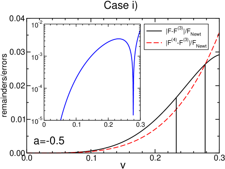
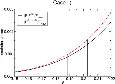
Figure 3: Left: absolute value of the remainder of the $N=3$ PN flux, $|F-F^{(3)}|/F_{\rm Newt}$ (solid line), and the $N=4$ term $|F^{(4)}-F^{(3)}|/F_{\rm Newt}$ (dashed red line). The inset shows the modulus of their difference, Eq. (8), in a semilogarithmic scale. Right: same as the left panel, but for the $N=6$ remainder and $N=7$ term. All curves in this plot refer to the counterrotating case with spin $a=-0.5$. The lower ($v_{l}$, more conservative) and upper ($\bar{v}$, less conservative) edges of the region of validity are (somewhat conventionally) delimited by the vertical lines, as explained in the main text.

This figure provides some clues about the edge of the region of validity of the PN approximation. For corotating orbits (left panel of Fig. 2), as the spin increases from zero to $a=0.9$, the higher-order PN approximants start to deviate from numerical results at lower values of $v/v_{{\mbox{\tiny ISCO}}}$: this happens roughly when $v/v_{{\mbox{\tiny ISCO}}}\simeq 0.6$ for $a=0$, and when $v/v_{{\mbox{\tiny ISCO}}}\simeq 0.4$ for $a=0.9$. This leads us to naively expect a shrinking of the region of validity of the PN approximation as a function of positive $a$. This expectation will be validated (at least qualitatively) in Section III: cf. the bottom-right panel of Fig. 4 below.

At first sight, the results for counterrotating orbits (right panel of Fig. 2) seem surprisingly good. In particular, the 3PN approximation (dash-dot-dotted, orange line) is almost indistinguishable from the numerical result all the way up to $v=v_{{\mbox{\tiny ISCO}}}$ when the spin is large. Such a good performance is simply because of the well-known, monotonically-increasing behavior of $v_{{\mbox{\tiny ISCO}}}$ with spin, with a minimum as $a\to-1$ (cf. Fig. 1). Since counterrotating orbits probe a smaller range in $v/c$ (up to $v/c\sim 0.35$ for fast-spinning BHs), the PN approximation is more accurate. Unfortunately, prograde accretion is likely to be more common than retrograde accretion in astrophysical settings (see e.g. Berti:2008af ). Moreover, the 3.5PN and 4PN approximants are significantly worse than the 3PN one at $a=-0.99$. This is consistent with the PN series being an asymptotic expansion, as one of the characteristic features of the latter is that beyond a certain optimal order, higher-order approximants become less accurate Bender:1978 .

III Region of validity

Let us now turn to determining the region of validity of the PN approximation for different values of the BH spin. For a complete review of asymptotic approximation techniques we refer the reader to Bender:1978 ; Paper I presents a short introduction to the topic in the present context. As explained in those references, the edge of the region of validity is determined by the approximate condition

$${\cal{O}}(F-F^{(N)})={\cal{O}}(F^{(N+1)}-F^{(N)})\,,$$ (7)

where $F$ denotes the “true” (numerical) result for the GW energy flux and $F^{(N)}$ denotes the $N$-th order PN approximation.

An inherent and intrinsic ambiguity is contained in Eq. (7), encoded in the order symbol. This makes any definition of the region of validity of an asymptotic series somewhat imprecise. As shown in Fig. 3 (or in Fig. 8 of Paper I), there are two qualitatively different scenarios:

1. Left panel of Fig. 3: The next-order term $|F^{(N+1)}-F^{(N)}|$ starts off smaller than the remainder $|F-F^{(N)}|$, but eventually they cross and separate. We can then estimate the edge of the region of validity $\bar{v}$ by solving $\delta^{(N)}(\bar{v})=0$, where

   $$\delta^{(N)}(v)\equiv\left||F-F^{(N)}|-|F^{(N+1)}-F^{(N)}|\right|\,$$ (8)

   is the error function. If we also define a more conservative lower edge of the region of validity, $v_{l}$, as the point where

   $$\left.\frac{d\delta^{(N)}(v)}{dv}\right|_{v_{l}}=0\,,$$ (9)

   we can then introduce an uncertainty width of the region of validity: $\delta\bar{v}\equiv\bar{v}-v_{l}$; see the inset of the left panel of Fig. 3.

2. Right panel of Fig. 3: The remainder and the next-order term are of the same order for sufficiently low velocities, until eventually the curves separate for larger velocities. This situation is the rule, rather than the exception, for the problem we consider in this paper. When this happens, method i) cannot be applied, because $\delta^{(N)}(v)=0$ has no solutions. Given the approximate nature of the order relationship in Eq. (7), we can define the region of validity as the point $\bar{v}$ such that $\delta^{(N)}(\bar{v})=\delta_{0}$, where $\delta_{0}$ is some given tolerance defined below.

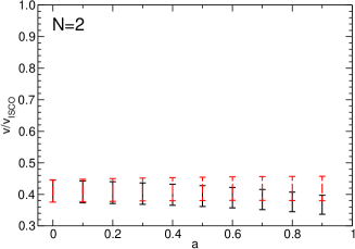
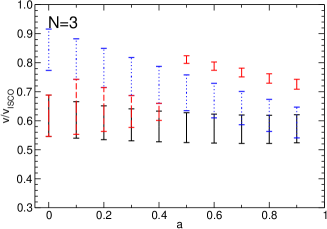
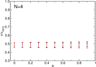
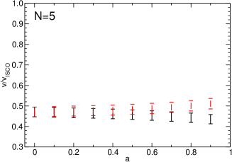
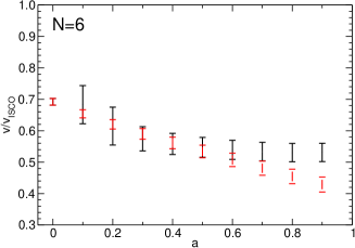
Figure 4: Edge of the region of validity as a function of $a$ for different PN orders, in the corotating (black, straight line) and counterrotating (red, dashed line) cases. The blue, dashed lines for $N=3$ refer to the counterrotating case, and they were obtained by an alternative method (see the discussion around Fig. 7 below).

Higher-order approximations should be sensitive to a smaller tolerance, which implies that $\delta_{0}$ cannot be set arbitrarily. Instead, $\delta_{0}$ should be given by the error in the difference between the $N$th remainder and the $(N+1)$th-order term. This error is presumably of the order of the error in the $(N+1)$th-order term, and it can be estimated by the $(N+2)$th-order term. The imprecision of the order symbol is now encoded in the fact that $\delta_{0}$ depends on $v$. We can try to estimate its value by evaluating the $(N+2)$th order term in the middle of the allowed range, that is, at $v_{{\mbox{\tiny ISCO}}}/2$:

$$\delta_{0}=\left|F^{(N+2)}(v_{{\mbox{\tiny ISCO}}}/2)-F^{(N+1)}(v_{{\mbox{\tiny ISCO}}}/2)\right|\,.$$ (10)

This estimate of $\delta_{0}$ is not exact, so we can try to provide a more conservative lower edge of the region of validity, $v_{l}$, by imposing the condition $\delta^{(N)}(v_{l})=\delta_{0}/2$. We can then define an uncertainty on the region of validity $\delta\bar{v}=|\bar{v}-v_{l}|$. This is illustrated pictorially by the vertical lines in the right panel of Fig. 3.

Let us now discuss the behavior of the edge of the region of validity as a function of the PN order $N$ and of the BH spin $a$. The corotating and counterrotating regions of validity and the associated errors are shown in Fig. 4 with solid black (dashed red) error bars for corotating (counterrotating) orbits, respectively.

Let us first consider the corotating case (solid black error bars). All results were obtained using method ii) above. At any fixed PN order, the normalized region of validity $v/v_{{\mbox{\tiny ISCO}}}$ remains roughly constant as a function of $a$. With a few exceptions, the most conservative estimate $v_{l}$ (lower edge of the error bars in the plots) is typically in the range $v/v_{{\mbox{\tiny ISCO}}}\in[0.3\,,0.6]$. This is consistent with the left panel of Fig. 2, where we see that all PN approximations (including high-order ones) peel off from the numerical flux in this range.

These figures allow us to arrive at an interesting conclusion. When we recall that $v_{{\mbox{\tiny ISCO}}}$ increases with $a$ (cf. Fig. 1), the figures suggest that spin-dependent corrections in the PN expansion of Eq. (1) are effective at pushing the validity of the PN expansion to higher values of $v/c$. However, there is an intrinsic limit to what is achievable, which is determined instead by $v/v_{{\mbox{\tiny ISCO}}}$, and roughly independent of $a$. In the range $a\in[0.3\,,0.9]$, $v_{{\mbox{\tiny ISCO}}}$ increases from $\simeq 0.444$ to $\simeq 0.609$. Therefore the region of validity for the orbital velocity is approximately in the range $v/c\in[0.44\times 0.3\,,0.61\times 0.6]\sim[0.13\,,0.37]$.

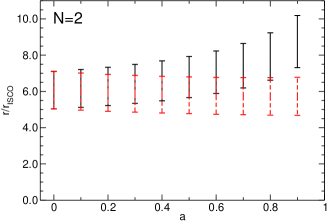
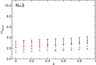
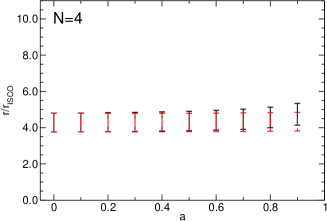
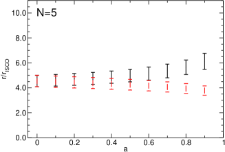
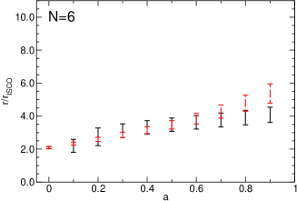
Figure 5: Edge of the region of validity expressed in terms of the Boyer-Lindquist radius for different PN orders, in the corotating (black, straight line) and counterrotating (red, dashed line) cases. The blue, dashed lines for $N=3$ refer to the counterrotating case, and they were obtained by an alternative method (see the discussion around Fig. 7 below).

Let us now focus on the counterrotating case, i.e. on the dashed red error bars in Fig. 4, which, again, were determined using method ii) above. The only exception is the case $N=3$ (corresponding to the right panel of Fig. 3), that we will discuss separately below. As in the corotating case, the region of validity shrinks mildly or remains roughly constant as $|a|$ increases. For $N=6$ the region of validity shrinks faster with increasing spin.

The edge of the region of validity can also be presented in terms of the Boyer-Lindquist radius of the particle’s circular orbit. The corresponding plots for the corotating and counterrotating cases are presented, for completeness, in Fig. 5. The ISCO radius $r_{{\mbox{\tiny ISCO}}}$ is a monotonically decreasing function of the spin (or of $v_{{\mbox{\tiny ISCO}}}$), so, quite naturally, the trend as a function of $a$ is the opposite of what we observed for velocities in Fig. 4. Our results consistently suggest that the region of validity of the PN approximation cannot be extended all the way down to the ISCO, contrary to a rather common assumption in GW data analysis. Instead, one should use care when using, for example, the 2PN approximation for $r/r_{{\mbox{\tiny ISCO}}}<4$, as in that regime higher-order PN terms cannot be neglected (this is particularly true for rapidly rotating BHs in prograde orbits). Our results suggest that a safer choice would be to truncate all analyses at $r/r_{{\mbox{\tiny ISCO}}}=6$, which ranges between $r/M\in[6\,,54]$ depending on the BH spin, unless one is dealing with approximants more accurate than Taylor expansions.

Finally, one can also investigate how the edge of the region of validity behaves with PN order. This is depicted in Fig. 6 for a set of fixed values of $a$ (shown with different colors, as described in the caption). The vertical dashed lines separate the different-$N$ orders. If we concentrate on the nonspinning case (black), ignore the pathological case $N=3$ (discussed below) and consider the conservative, lower end of the error bar, we see that there is a maximum at $N=6$. For larger values of $N$, $v/v_{{\mbox{\tiny ISCO}}}$ would consistently decrease, as found in Paper I. In the spinning case, however, this trend is not as clear, as at $N=6$ the edge of the region of validity is rather sensitive to the spin value. Without higher-order terms in the PN expansion, which would provide larger-$N$ points in this figure, one cannot conclude whether $N=6$ is the optimal order of expansion in the spinning case.

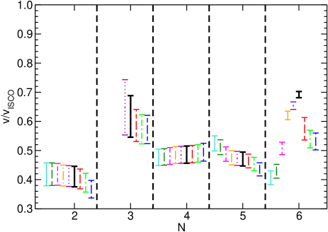
Figure 6: Edge of the region of validity as a function of $N$ for fixed values of $a$. The thick, black error bar corresponds to $a=0$, followed by $a=0.3\,,0.6\,,0.9$ to the right and $a=-0.1\,,-0.2\,,-0.6\,,-0.9\,,-0.99$ to the left. Note that $N=3$ is a special case. For reasons discussed in the text, we do not give error bars for $N=3$ and $a<-0.1$.

Before moving on to the next Section, let us discuss the $N=3$ case for counterrotating orbits in more detail. This is a special case, as noted by the discontinuity in counterrotating orbits shown in Figs. 4, 5. The pathologies explained below are the reason why, in Fig. 6, we only plotted the counterrotating edge of the region of validity when the Kerr spin parameter $|a|\leq 0.1$. Notice also that, when $N=3$, the error regions in Fig. 6 are significantly larger than for any other $N$ value. We will discuss the reason for this below, but the impatient reader can skip to the next section without loss of continuity.

Figure 7 clarifies the origin of the problem. When we use method ii), the top margin of the edge of the region of validity is estimated as the (smallest) value of $\bar{v}/v_{{\mbox{\tiny ISCO}}}$ for which $\delta^{(3)}(\bar{v})=\delta_{0}$. This condition corresponds to the leftmost intersection of the horizontal dashed red line with the solid black line in the plot. Similarly, we determine the most conservative estimate of the edge of the region of validity by considering the smallest $v_{l}$ such that $\delta^{(3)}(v_{l})=\delta_{0}/2$. This corresponds to the leftmost intersection of the horizontal, dot-dashed green line with the solid black line. For corotating orbits, as it happens, these intersections always exist. In fact, the local maximum in $\delta^{(3)}(v)$ (which is located at $v/v_{{\mbox{\tiny ISCO}}}\sim 0.8$ for $a=0$) moves to the right and becomes significantly larger as $a\to 1$. For counterrotating orbits the trend is the opposite: the local maximum moves to the left and decreases in magnitude. For a critical value of the spin $a\simeq-0.1$, the red dashed line and the solid black line do not intersect anymore. This is why in Figs. 4 and 5 we only plot the red-dashed (counterrotating) edge of the region of validity when $|a|\leq 0.1$. Of course, we can insist to identify $\bar{v}$ and $v_{l}$ as the smallest values of $v$ such that $\delta^{(3)}(\bar{v})=\delta_{0}$, $\delta^{(3)}(v_{l})=\delta_{0}/2$. This procedure leads to the red, dashed error bars in the $N=3$ panel of Figs. 4 and 5. Note that these error bars are unnaturally small for $|a|>0.4$.

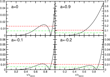
Figure 7: The solid black line shows $\delta^{(N)}(v)$ for $N=3$. The horizontal dashed red (dot-dashed green) lines represent $\delta_{0}$, computed from Eq. (10), and $\delta_{0}/2$. See text for discussion.

Another possible solution would be to switch to method i) when method ii) fails. Now the upper margin of the edge of the region validity would be given by the first zero of $\delta^{(3)}(v)$, and the lower margin would be estimated by the condition given in Eq. (9). This results in the blue, dotted error bars shown in the central top panel of Figs. 4 and 5. These error bars are significantly more optimistic than the ones we presented in the rest of the paper, but (in our opinion) their significance is not as clear and well-justified as the rest of our results.

The problem discussed in this section concerns counterrotating orbits and $N=3$. This is an exceptional case, and it does not affect the conclusions drawn earlier in the paper. However we should remark, for completeness, that similar pathologies occur for corotating orbits with $N=6$ when $0\leq a\leq 0.2$, and they may also occur at higher PN orders.

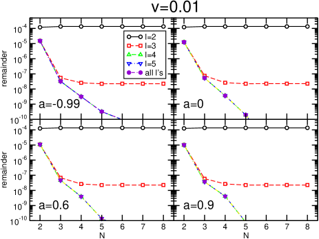
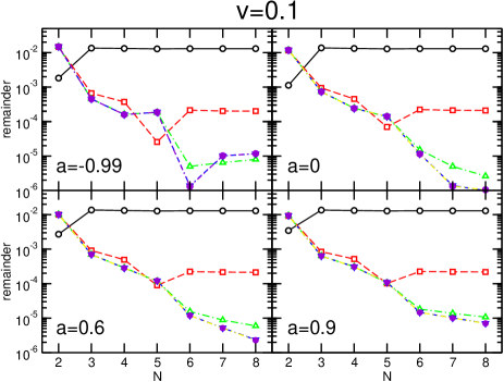
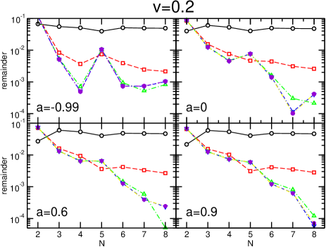
Figure 8: Relevance of multipolar components up to $\ell=2$, $\ell=3$, $\ell=4$, $\ell=5$, and summing as many $\ell$’s as necessary for the relative accuracy of the Teukolsky code to be ${\cal O}(10^{-10})$ at any given velocity.

IV Relevance of multipolar components as a function of spin

Until now, we compared the PN approximation to numerical results that were considered to be virtually “exact”. This was justified because the Teukolsky code computes as many multipoles in the angular decomposition of the radiation as needed to achieve an accuracy of ${\cal{O}}(10^{-10})$ at any given orbital velocity. While this is manageable in frequency-domain calculations, sometimes accurate calculations of a large number of multipoles are not possible in extreme mass-ratio time-domain codes, or in numerical relativity simulations of comparable-mass binaries: cf. Berti:2007fi ; Berti:2007nw for an analysis of multipolar decompositions of the radiation from comparable-mass binaries and Pollney:2009yz ; Pollney:2010hs for more recent numerical work to overcome these difficulties. As advocated in several papers Yunes:2008tw ; Damour:2008gu ; Bernuzzi:2010xj ; 2009GWN…..2….3Y ; Yunes:2009ef ; Yunes:2010zj ; Pan:2010hz , EMRIs provide a simple playground to study the number of multipolar components required to reach a given accuracy in the PN approximation (or in one of its resummed variants).

Figure 8 shows a comparison of the convergence of the multipolar decomposition versus the convergence of the PN expansion of the energy flux. This plot generalizes Fig. 7 of Paper I in two ways: (i) it uses more accurate numerical data, and (ii) it considers the effect of the central BH spin on the number of multipolar components required to achieve a given accuracy.

We fix three values of the orbital velocity ($v=0.01$, $v=0.1$ and $v=0.2$) and we plot $F^{(\ell)}-F^{(N)}$, where $F^{(N)}$ is the $N$th approximant of the PN energy flux and $F^{(\ell)}$ is the numerical energy flux truncated at the $\ell$th angular multipole. Some features are immediately visible from this plot:

• Even at low orbital velocities ($v=0.01$), it is necessary to include multipolar components up to and including $\ell=4$ to achieve an accuracy better than $10^{-7}$ in the flux; on the other hand, including up to $\ell=5$ we obtain results that are as accurate as those that would be obtained including more multipoles.

• For an orbital velocity $v=0.1$ ($v=0.2$) the best-known PN flux and numerical calculations always disagree at levels of $\sim 10^{-6}$ ($\sim 10^{-4}$) or larger. This is obviously due to the slower, nonmonotonic convergence of the PN approximation in this regime. Some nontrivial features of the PN approximation are again well-visible here: for example, as pointed out repeatedly in this paper, when $a=-0.99$ and $v=0.1$ the 3PN ($N=6$) expansion performs much better than higher-order expansions. This may well be accidental, and in fact it does not hold when $v=0.2$, as then $N=4$ is (most likely accidentally) better.

• As a rule of thumb, the inclusion of multipoles up to and including $\ell=5$ seems necessary to achieve the level of accuracy of the best-known ($N=8$) PN expansion of the flux in the Kerr case. This conclusion is independent of the spin parameter $a$. In fact, $a$ has hardly any effect on the number of multipolar components that must be included in the flux to achieve a desired accuracy.

V Conclusions

We extended the method proposed in Paper I to determine the formal region of validity of the PN approximation for quasicircular EMRIs of compact objects in the equatorial plane of a Kerr BH. The boundary of the formal region of validity is defined as the orbital velocity where the “true” error in the approximation (relative to high-accuracy numerical calculations) becomes comparable to the series truncation error (due to neglecting higher-order terms in the series).

For quasicircular, equatorial Kerr EMRIs, the PN expansion is known up to 4PN, and our estimate of the region of validity can only be pushed up to 3PN. Our main results are shown in Fig. 4 (in terms of orbital velocity) and in Fig. 5 (in terms of orbital radius). At fixed but arbitrary spin parameter $a$, the 3PN approximation has no obvious advantage when compared with other PN orders. At fixed PN order $N$, Fig. 4 shows an interesting trend: when normalized by the ISCO velocity $v_{{\mbox{\tiny ISCO}}}$, to a very good approximation the region of validity does not depend on $a$.

We should emphasize that our results say nothing about the absolute accuracy of the PN approximation: they only suggest relational statements between the $N$th and the $(N+1)$th-order approximations. For velocities within the region of validity of the asymptotic series, all we can say is that the $N$th order approximation has errors that are of expected relative size. For larger velocities, the $(N+1)$th- and higher-order terms become important, and should not be formally neglected. If we can tolerate errors larger than those estimated by the $(N+1)$th order term (at the risk that higher-order approximations may be less accurate than lower-order ones) we can surely use the PN expansion beyond the realm of its formal region of validity. This, however, would force us to lose analytic control of the magnitude of the error, as given by the next order term. The meaning of this caveat is well illustrated by the counterrotating case with $a=-0.99$: it is clear from Fig. 2 that the 3.5PN and 4PN approximations do not represent an improvement over the 3PN approximation (and in fact perform quite badly) beyond the realm of the region of validity.

Future work could concentrate on studying whether resummation techniques, such as Padé Damour:1997ub ; Damour:2000zb ; Mroue:2008fu or Chebyshev Porter:2007vk , enlarge the formal region of validity, using the methods developed here. This would allow us to identify optimal resummation methods, which, in turn, affects resummed waveform models for EMRIs, like the effective-one-body approach 2009GWN…..2….3Y ; Yunes:2009ef ; Yunes:2010zj . Moreover, one could attempt to establish whether there is a correlation between the accuracy of the energy flux, as measured by the asymptotic methods developed here, and the accuracy of the waveform model, as required by GW detectors.

Note added in proof. After submission of this paper, we learned that Fujita has extended PN calculations of the energy flux up to 14PN for nonrotating (Schwarzschild) BHs Fujita:2011zk .

- (1) Bender, C. M., & Orszag, S. A. 1978, Advanced Mathematical Methods for Scientists and Engineers, New York: McGraw-Hill, 1978.
- (2) N. Yunes, E. Berti, Phys. Rev. D77, 124006 (2008). [arXiv:0803.1853 [gr-qc]].
- (3) E. Poisson, Phys. Rev. D52, 5719-5723 (1995). [gr-qc/9505030].
- (4) H. Tagoshi, M. Shibata, T. Tanaka, M. Sasaki, Phys. Rev. D54, 1439-1459 (1996). [gr-qc/9603028].
- (5) T. Tanaka, H. Tagoshi, M. Sasaki, Prog. Theor. Phys. 96, 1087-1101 (1996). [gr-qc/9701050].
- (6) N. Yunes, GW Notes, Vol. 2, p. 3-47 (2009).
- (7) N. Yunes, A. Buonanno, S. A. Hughes, M. Coleman Miller, Y. Pan, Phys. Rev. Lett. 104, 091102 (2010). [arXiv:0909.4263 [gr-qc]].
- (8) N. Yunes, A. Buonanno, S. A. Hughes, Y. Pan, E. Barausse, M. C. Miller, W. Throwe, Phys. Rev. D83, 044044 (2011). [arXiv:1009.6013 [gr-qc]].
- (9) Y. Mino, M. Sasaki, M. Shibata, H. Tagoshi, T. Tanaka, Prog. Theor. Phys. Suppl. 128, 1-121 (1997). [gr-qc/9712057].
- (10) Y. Pan, A. Buonanno, R. Fujita, E. Racine, H. Tagoshi, Phys. Rev. D83, 064003 (2011). [arXiv:1006.0431 [gr-qc]].
- (11) J. M. Bardeen, W. H. Press, S. A. Teukolsky, Astrophys. J. 178, 347 (1972).
- (12) T. Damour, B. R. Iyer, B. S. Sathyaprakash, Phys. Rev. D57, 885-907 (1998). [gr-qc/9708034].
- (13) T. Damour, B. R. Iyer, B. S. Sathyaprakash, Phys. Rev. D63, 044023 (2001). [gr-qc/0010009].
- (14) A. H. Mroue, L. E. Kidder, S. A. Teukolsky, Phys. Rev. D78, 044004 (2008). [arXiv:0805.2390 [gr-qc]].
- (15) E. K. Porter, Phys. Rev. D76, 104002 (2007). [arXiv:0706.0114 [gr-qc]].
- (16) E. Berti, M. Volonteri, Astrophys. J. 684, 822-828 (2008). [arXiv:0802.0025 [astro-ph]].
- (17) E. Berti, V. Cardoso, J. A. Gonzalez, U. Sperhake, M. Hannam, S. Husa, B. Bruegmann, Phys. Rev. D76, 064034 (2007). [gr-qc/0703053 [GR-QC]].
- (18) E. Berti, V. Cardoso, J. A. Gonzalez, U. Sperhake, B. Bruegmann, Class. Quant. Grav. 25, 114035 (2008). [arXiv:0711.1097 [gr-qc]].
- (19) D. Pollney, C. Reisswig, E. Schnetter, N. Dorband, P. Diener, Phys. Rev. D83, 044045 (2011). [arXiv:0910.3803 [gr-qc]].
- (20) D. Pollney, C. Reisswig, [arXiv:1004.4209 [gr-qc]].
- (21) T. Damour, B. R. Iyer, A. Nagar, Phys. Rev. D79, 064004 (2009). [arXiv:0811.2069 [gr-qc]].
- (22) S. Bernuzzi, A. Nagar, A. Zenginoglu, Phys. Rev. D83, 064010 (2011). [arXiv:1012.2456 [gr-qc]].
- (23) R. Fujita, [arXiv:1104.5615 [gr-qc]].