A LOW-REYNOLDS-NUMBER TREADMILLING SWIMMER NEAR A SEMI-INFINITE WALL

Abstract

We investigate the behavior of a treadmilling microswimmer in a two-dimensional unbounded domain with a semi-infinite no-slip wall. The wall can also be regarded as a probe or pipette inserted into the flow. We solve the governing evolution equations in an analytical form and numerically calculate trajectories of the swimmer for several different initial positions and orientations. We then compute the probability that the treadmilling organism can escape the vicinity of the wall. We find that many trajectories in a ‘wedge’ around the wall are likely to escape. This suggests that inserting a probe or pipette in a suspension of organism may push away treadmilling swimmers.

1 Introduction

The locomotion of microorganisms is an active research area of fluid dynamics and biology (see for instance the reviews [10, 15]). As their motion occurs on very small length scales and speeds, their dynamics is governed by low-Reynolds-number hydrodynamics, where inertial forces are negligible in comparison to the viscous effects of the fluid (Stokes flow).

Many studies deal with such dynamics in unbounded or very large domains [18, 12, 1]. In reality, however, most organisms are in the vicinity of other bodies or boundaries, where hydrodynamic interactions can have a significant effect on their motion. The importance of boundaries has also been suggested by experimental observations. For example, some research suggests that microorganisms are attracted to solid walls [17, 19, 3]. Berke et al. [2] measured the steady-state distribution of E. Coli bacteria swimming between two glass plates and found a strong increase of the cell concentration at the boundaries. They also theoretically demonstrated that hydrodynamic interactions of swimming cells with solid surfaces lead to their reorientation in the direction parallel to the surfaces. Lauga et al. [9] showed that circular trajectories are natural consequences of force-free and torque-free swimming and hydrodynamic interactions with the boundary. This leads to a hydrodynamic trapping of the cells close to the surface. Drescher et al. [6] found that when two nearby Volvox colonies swim close to a solid surface, they attract one another and can form stable bound states in which they ‘waltz’ or ‘minuet’ around each other. These observations suggest that, in order to obtain a comprehensive understanding of low-Reynolds-number locomotion, it is necessary to study hydrodynamic interactions between microorganisms and boundaries.

Some of the phenomena stated above have already been confirmed by numerical simulations [16, 8]. However, not many physical explanations have been given to the locomotion of microorganism near boundaries. Berke et al. [2] have captured the swimming microorganisms’ attraction to boundaries by modeling the swimmer as a force dipole singularity. However, contrary to the experimental findings, the microorganism in this model crashes into the boundary in finite time. Or and Murray [14] studied the dynamics of low-Reynolds-number swimming organism near a plane wall. They analyzed the motion of a swimmer consisting of two rotating spheres connected by a thin rod as a simple theoretical model of a ‘treadmilling’ swimming organism. They found that when the spheres rotate with different velocities their model has a solution with steady translation parallel to the wall, and that under small perturbation the swimmer exhibits a ‘bouncing’ motions parallel to the wall. These results have recently been verified experimentally on a macroscale robotic prototype swimming in a highly viscous fluid [20]. Furthermore, Crowdy and Or [4] have proposed a singularity model for swimming microorganisms placed near an infinite no-slip boundary. Their model was based on a circular treadmilling organism which has no means of self-propulsion, that is, the organism doesn’t move unless it interacts with a boundary. (For example, the organism may be creating a feeding current.) They proposed an appropriate Stokes singularities that represent the flow field created by this treadmilling organism. By studying the interaction between these singularities and the no-slip wall, they formulated explicit evolution equations for the motion of the organism, and fully characterized its motion near the wall. They found trajectories with a periodic bouncing motion along the wall which had remarkable similarity to the trajectories shown in Or and Murray [14]. Crowdy and Samson [5], using the point-singularity model, investigated the dynamics of treadmilling organism near an infinite no-slip boundary with a gap of a fixed size. They employed a conformal mapping technique to avoid the difficulty in treating the image of the treadmilling organism on the wall. They found that the treadmilling organism can exhibit several qualitatively different types of trajectories: jumping over the gap, rebounding from the gap, being trapped near the gap, and escaping the gap region even when the organism has initial position in the gap. They also performed a bifurcation analysis in terms of the model parameters, and demonstrated the presence of stable equilibrium points in the gap region as well as Hopf bifurcations to periodic bound states. This reduced model also exhibited a global gluing bifurcation in which two symmetric periodic orbits merge at a saddle point into symmetric bound states having more complex spatio-temporal structure.

In the present paper we examine the dynamics of a treadmilling organism near a semi-infinite no-slip wall, modeled as a flat plate of zero thickness. Though this is a special case of the model of Crowdy and Samson [5], it deserves separate investigation because of the simpler equations involved, and because the semi-infinite wall can be regarded as a probe or pipette inserted in the system, a common situation in microbiology. We also analyze the trajectories in a very different manner to [5], as we attempt to quantify the probability of escape from the wall’s vicinity, assuming the treadmillers are randomly oriented.

2 Model of a treadmilling microorganism

Following previous authors [4, 5], we consider a two-dimensional model for a microorganism in the $(x,y)$-plane, which we treat as the complex plane with $z\equiv x+iy$. Our derivation is a special case of [5], who considered a microswimmer near a slit or gap in an infinite wall. Nevertheless, as mentioned in the introduction, the semi-infinite wall is important enough to be treated separately, as it arises in the neighborhood of a probe or a pipette.

The Stokes equations which describe the motion of an incompressible viscous fluid are

$$\nabla p=\eta\Delta\bm{u},\qquad\nabla\cdot\bm{u}=0,$$ (1)

where $\Delta$ is the Laplace operator, $\bm{u}=(u_{x},u_{y})$ is the fluid velocity, and $p$ and $\eta$ are the pressure and dynamic viscosity, respectively. As we are considering a two-dimensional flow, we can introduce a stream function $\psi$, such that the velocity is given by $u_{x}=\partial\psi/\partial y$, $u_{y}=-\partial\psi/\partial x$. Then the Stokes equations (1) reduce to the biharmonic equation $\Delta^{2}\psi=0$. The complex velocity is $W=u_{x}+iu_{y}=-2i{\partial\psi}/{\partial{\bar{z}}}$, with

$$W =u_{x}+iu_{y}=-2i\frac{\partial\psi}{\partial{\bar{z}}}=f(z)+z\overline{f^{\prime}(z)}+\overline{g^{\prime}(z)},$$ (2)

$$\psi ={\rm Im}[{\bar{z}}f(z)+g(z)].$$ (3)

where $f(z)$ and $g(z)$ are called Goursat functions; they are analytic everywhere in the flow domain, except where isolated singularities are introduced to model swimmers. For a treadmilling swimmer, we take $f(z)$ to have a simple pole at $z=z_{d}$, so that

$$f(z)=\frac{\mu}{z-z_{d}}+\ldots,\qquad g^{\prime}(z)=\frac{\mu\bar{z}_{d}}{(z-z_{d})^{2}}+\ldots.$$ (4)

where $\mu\in\mathbb{C}$ and the form of $g^{\prime}$ is forced by the requirement that the complex velocity (2) have no higher than a $|z-z_{d}|^{-1}$ singularity. This solution corresponds to a stresslet of strength $\mu$ at $z_{d}$. The ellipses in (4) indicate analytic terms. The expansion (4) is the basic solution for a treadmilling swimmer, which does not have any self-propulsion in itself, but can move due to its interaction with boundaries [11, 14, 20, 4, 5].

In a simple model, we assume that the treadmilling organism has a circular body of radius $\epsilon$, with a center at $z_{d}(t)=x_{d}(t)+iy_{d}(t)$. We also assume that, with respect to the angle $\theta(t)$ of the head of the treadmilling organism from the real axis, surface actuators of the treadmilling organism induce a tangential velocity profile given by [4]

$$U(\phi,\theta)=2V\sin(2(\phi-\theta)),$$ (5)

where $V$ is a constant and $\phi$ is the angle measured from the positive $x$ direction.

Next consider the treadmiller near an infinite wall along the $x$ axis. To satisfy the no-slip boundary condition at the wall, we make the expansion

$$\begin{split}f(z,t)&=\frac{\mu}{z-z_{d}(t)}+f_{0}+(z-z_{d}(t))f_{1}+\cdots,\\ g^{\prime}(z,t)&=\frac{b}{(z-z_{d}(t))^{3}}+\frac{a}{(z-z_{d}(t))^{2}}+g_{0}+\cdots,\end{split}$$ (6)

$f(z,t)$ having no Stokeslet term and $g(z,t)$ having no rotlet term implying that the treadmilling organism is force-free and torque-free. We use the boundary condition to find

$$\mu=-i\epsilon\overline{c},\qquad a=\mu{\bar{z}}_{d},\qquad b=\mu\epsilon^{2}-i\overline{c}\epsilon^{3}=2\mu\epsilon^{2},$$ (7)

where $c(t)\equiv-iV\exp(-2i\theta(t))$. We set the time scale of the motion by letting $V=\epsilon^{-1}$ so that $\mu(t)=\exp(2i\theta(t))$. The coefficients $f_{0}$, $f_{1}$, and $g_{0}$ are given in [4].

The time derivative of the position and orientation of the treadmilling organism is obtained by equating the time rate of change of position to the local fluid velocity, and the time rate of change of orientation to half the local vorticity:

$$\frac{dz_{d}}{dt}=-f_{0}+z_{d}{\bar{f}}_{1}+{\bar{g}}_{0},\qquad\frac{d\theta}{dt}=-2\,{\rm Im}\,f_{1}.$$ (8)

Equation (8) can then be solved as a set of three ODEs determining the motion of the treadmiller.

Now we turn to a semi-infinite wall, extending along the negative $x$ axis. The conformal mapping $\zeta=iz^{1/2}$ maps the $z$ plane to upper-half $\zeta$ plane, with the negative $x$-axis of the $z$ plane mapped to the real axis in the $\zeta$ plane. In the $\zeta$ plane we can use a similar singular expansion as (6), but we must take care to map the boundary conditions to the $\zeta$ plane. We omit the lengthy details, which are similar to Crowdy and Samson [5]. See [13] for a more complete derivation. All that is required for simulating the swimmer trajectories are the coefficients that appear in (8), which are

$$f_{0}=\frac{\mu}{4z_{d}}-\frac{\epsilon^{2}{\bar{\mu}}}{4\mathcal{Z}^{3}{\bar{z}}_{d}^{3/2}}+\frac{\left(2|z_{d}|^{2}-2{\bar{z}}_{d}^{2}-3\epsilon^{2}\right){\bar{\mu}}}{8\mathcal{Z}^{2}{\bar{z}}_{d}^{2}}+\frac{\left(2|z_{d}|^{2}+2{\bar{z}}_{d}^{2}-3\epsilon^{2}\right){\bar{\mu}}}{8\mathcal{Z}{\bar{z}}_{d}^{5/2}},$$ (9a)

$$f_{1}=\frac{1}{12z_{d}^{2}}\biggl{(}-\frac{3\mu}{4}+\frac{9z_{d}^{3/2}\epsilon^{2}{\bar{\mu}}}{2\mathcal{Z}^{4}{\bar{z}}_{d}^{3/2}}-\frac{3z_{d}^{3/2}\left(2|z_{d}|^{2}-2{\bar{z}}_{d}^{2}-3\epsilon^{2}\right){\bar{\mu}}}{2\mathcal{Z}^{3}{\bar{z}}_{d}^{2}}\\ -\frac{3z_{d}^{3/2}\left(2|z_{d}|^{2}+2{\bar{z}}_{d}^{2}-3\epsilon^{2}\right){\bar{\mu}}}{4\mathcal{Z}^{2}{\bar{z}}_{d}^{5/2}}\biggr{)},$$ (9b)

and

$$g_{0}=-\frac{3\mu{\bar{z}}_{d}}{16z_{d}^{2}}+\frac{10\epsilon^{2}\mu}{32z_{d}^{3}}+\frac{3\epsilon^{2}{\bar{\mu}}}{8\mathcal{Z}^{4}{\bar{z}}_{d}}-\frac{\left(z_{d}-{\bar{z}}_{d}\right){\bar{\mu}}}{4\mathcal{Z}^{3}{\bar{z}}_{d}^{1/2}}\\ +\frac{\left(2|z_{d}|^{2}-6{\bar{z}}_{d}^{2}-3\epsilon^{2}\right){\bar{\mu}}}{16\mathcal{Z}^{2}{\bar{z}}_{d}^{5/2}}\left({\bar{z}}_{d}^{1/2}+\mathcal{Z}\right),$$ (9c)

where $\mathcal{Z}\equiv z_{d}^{1/2}+{\bar{z}}_{d}^{1/2}$.

3 Results of numerical simulations

We now present the results of numerical simulations of the governing evolution equations (8), together with the coefficients (9c). The radius of the circular treadmillers is set to $\epsilon=1$, giving the reference length scale. The time scale is set by $V=\epsilon^{-1}$ in (5).

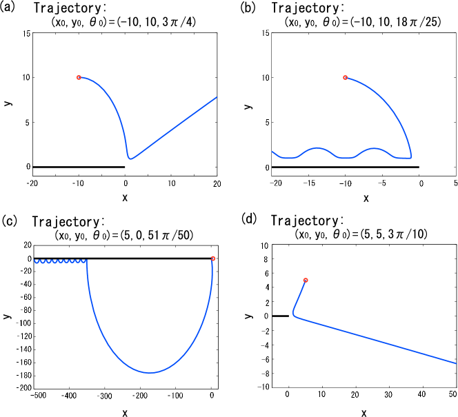
Figure 1: Examples of trajectories from the initial points $(x_{d0},y_{d0})$ marked with circles, with an initial orientation $\theta_{0}$. A treadmilling organism can escape from the wall, such as in (a) and (d), end up above the wall as in (b), or underneath the wall as in (c).

Figure 1 shows examples of swimmer trajectories for different initial conditions for position $z_{d0}$ and angle $\theta_{0}$. Some trajectories, such as (a) and (d), end up far away from the wall; we refer to those as escaping trajectories. Others, such as (b) and (c), remain close to the wall for all time, exhibiting the ‘bouncing’ behavior noted in [4]. A fourth type of trajectory (not shown) crashes into the wall, but this is an unphysical consequence of the boundary condition at the swimmer’s surface only being approximately satisfied. It has been verified numerically that the qualitative features of the trajectories are not affected by this approximation [7].

Both experimental observations and previous theoretical studies suggest that, when there is a no-slip wall near a treadmilling organism, the organism tends to be attracted to its own image and move towards the wall [17, 19, 9, 2, 16, 8, 4, 5]. This behavior is clearly seen at an early stage in all the trajectories in Fig. 1. Nevertheless, in the cases shown in Figs. 1(a) and (d), the treadmilling organism moves away from the wall after it has come close to the edge of the wall.

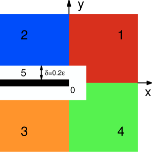
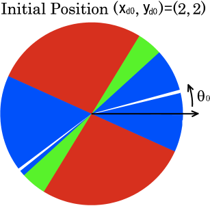
Figure 2: (a) The $x$–$y$ plane divided into five regions. The thick black line corresponds to the wall. (b) An example of a pie chart. The different colors as a function of initial orientation $\theta_{0}$ indicate which region of (a) the treadmilling organism ends up in after a sufficiently large time.

We now focus on the large-time behavior of treadmillers. To study this, we first introduce five regions shown in Fig. 2(a). Regions 1–4 are the usual quadrants of the plane, but with a neighborhood of size $0.2\epsilon$ around the wall removed; this removed neighborhood is region 5. The regions 1–5 are colored red, blue, orange, green, and white, respectively. From these regions, we can make a ‘pie chart’ around each point in the plane, an example of which is shown in Fig. 2(b). The sectors of the pie chart correspond to a range initial angle $\theta_{0}$; the color of the sector describes which region the treadmiller ends up in for large times (here $t=1500$). Region 5 corresponds to ‘crashing’ trajectories. Thus, for a given position, the treadmiller may end up in different regions, and the relationship between angle and final region is not simple.

Figure 3: Pie charts at $t=1500$ for several initial conditions. Each pie chart is centered on the initial condition it corresponds to. The thick black line represents the wall. Note that region 3 only appears as very thin slivers in the pie charts along the $x$ axis.

Figure 3 shows pie charts for many initial points $(x_{d0},y_{d0})$. The most notable feature is the complexity of the pie charts for initial points near the wall and with large negative $x$ coordinates. This reflects the fact that the treadmilling organism changes its heading direction and the quality of its trajectory significantly when it has come to the vicinity of the edge of the wall, $x=y=0$ depending upon its $(x_{d},y_{d},\theta)$ at the time, and so even a very small difference in initial condition can result in a huge difference to its trajectory. (This is an example of chaotic scattering.) However, pie charts tend to become rather simple for larger $y_{d0}$ for any fixed $x_{d0}$, since the treadmiller is then less influenced by the wall.

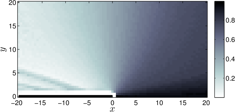
Figure 4: Escape probability $P_{E}$ at $t=1500$ for different initial points. Each point corresponds to a given initial condition $(x_{d0},y_{d0})$, integrated over all possible starting angles $\theta_{0}$. A trajectory escapes if it ends up in regions 1 or 4, as defined in Fig. 2. The excluded white area near the wall corresponds to initial conditions where the swimmer would be partially inside the wall.

Now let us consider the escape probability, $P_{E}(x_{d0},y_{d0})$, the probability that the treadmilling organism can escape from the wall region. We define this as the probability that the treadmilling organism be in region $1$ or $4$ at sufficiently large time. We assume that the initial angle $\theta_{0}$ is uniformly distributed. The escape probability $P_{E}(x_{d0},y_{d0})$ then corresponds to the fraction of angles in a pie chart that are red or green, for a given initial position $(x_{d0},y_{d0})$. The escape probability for $t=1500$ for different initial conditions is shown in Fig. 4, where each $(x,y)$ coordinate corresponds to an initial position of the treadmiller. Note that for almost all initial conditions there is some finite probability of escaping or being trapped, though the escaping probability approaches unity along the positive $x$ axis, and goes to zero for large negative $x$ and large $y$. Observe the strong ‘wedge’ of trajectories that are likely to escape ($P_{E}>0.6$), though there is also a backwards-facing wedge of trajectories that have a reasonable change of escaping ($P_{E}>0.3$). This suggests that a probe or pipette inserted in a medium is likely to ‘push away’ treadmillers to some degree. Note also the ‘tongues’ of abnormally-high ($P_{E}\simeq 0.4$) escape probability near the wall, which reflects the complicated structure of the pie charts in that region.

4 Discussion and conclusions

Following [4, 5], we derived the governing evolution equations for a treadmilling microorganism near a semi-infinite no-slip wall. This can also be regarded as a two-dimensional model of a probe or pipette inserted in the fluid. We then numerically calculated the trajectories of the organism for different initial conditions. The treadmilling organism was usually attracted to the wall for early times, but for later times often escaped the wall region. Typically this happened when the organism came close to the tip of the wall. To investigate this behavior further, we looked at ‘pie chart’ diagrams, where the sectors indicate which region a swimmer eventually ends up in as a function of its initial angular orientation. Initial points with larger negative $x$ coordinates have more complex pie charts compared to those with smaller negative $x$ coordinates, because they are sensitive to ‘chaotic scattering’ off the tip of the wall.

We then examined the escape probability $P_{E}$, the probability that the treadmilling organism can escape to the right of the wall region, assuming that it is initially randomly oriented. There is an evident ‘wedge’ of initial conditions that is likely to escape the wall. This suggests that a probe or pipette inserted could ‘push’ the organisms out of the way (with the wedge replaced by a cone in three dimensions), though since the organisms slow down as they get further away from the wall the effect might not be very pronounced.

References

- [1] J. E. Avron, O. Kenneth, and D. H. Oakmin, Pushmepullyou: an efficient micro-swimmer, New J. Phys., 7 (2005), p. 234.
- [2] A. P. Berke, L. Turner, H. C. Berg, and E. Lauga, Hydrodynamic attraction of swimming microorganisms by surfaces, Phys. Rev. E, 101 (2008), p. 038102.
- [3] J. Cosson, P. Huitorel, and C. Gagnon, How spermatozoa come to be confined to surfaces, Cell Motil. Cytoskel., 54 (2003), pp. 56–63.
- [4] D. G. Crowdy and Y. Or, Two-dimensional point singularity model of a low-Reynolds-number swimmer near a wall, Phys. Rev. E, 81 (2010), p. 036313.
- [5] D. G. Crowdy and O. Samson, Hydrodynamic bound states of a low-reynolds-number swimmer near a gap in a wall, (2010). Preprint.
- [6] K. Drescher, K. Leptos, I. Tuval, T. Ishikawa, T. J. Pedley, and R. E. Goldstein, Dancing volvox: hydrodynamic bound states of swimming algae, Phys. Rev. Lett., 102 (2009), p. 168101.
- [7] M. D. Finn. Private communication.
- [8] J. P. Hernandez-Ortiz, C. G. Dtolz, and M. D. Graham, Transport and collective dynamics in suspensions of confined swimming particles, Phys. Rev. Lett., 95 (2005), p. 204501.
- [9] E. Lauga, W. R. DiLuzio, G. M. Whitesides, and H. A. Stone, Swimming in circles: motion of bacteria near solid boundaries, Biophys. J., 90 (2006), pp. 400–412.
- [10] E. Lauga and T. R. Powers, The hydrodynamics of swimming micro-organisms, Rep. Prog. Phys., 72 (2009), p. 096601.
- [11] A. M. Leshansky, O. Kenneth, O. Gat, and J. E. Avron, A frictionless microswimmer, New J. Phys., 9 (2007), p. 145.
- [12] A. Najafi and R. Golestanian, Simple swimmer at low Reynolds number: Three linked spheres, Phys. Rev. E, 69 (2004), p. 062901.
- [13] K. Obuse, Trajectories of a low Reynolds number treadmilling organism near a half-infinite no-slip wall, in Proceedings of the 2010 Summer Program in Geophysical Fluid Dynamics, Woods Hole, MA, 2010, Woods Hole Oceanographic Institute.
- [14] Y. Or and R. M. Murray, Dynamics and stability of a class of low reynolds number swimmers near a wall, Phys. Rev. E, 79 (2009), p. 045302.
- [15] T. J. Pedley and J. O. Kessler, Hydrodynamic phenomena in suspensions of swimming microorganisms, Annu. Rev. Fluid Mech., 24 (1992), pp. 313–358.
- [16] M. Ramia, D. L. Tullock, and N. Phan-Thien, The role of hydrodynamics interaction in the locomotion of microorganism, Biophys. J., 65 (1993), pp. 755–778.
- [17] A. J. Rothschild, Non-random distribution of bull spermatozoa in a drop of sperm suspension, Nature, 198 (1963), pp. 1221–1222.
- [18] A. Shapere and F. Wilczek, Geometry of self-propulsion at low Reynolds numbers, J. Fluid Mech., 198 (1989), pp. 557–585.
- [19] H. Winet, G. S. Bernstein, and J. Head, Observations on the response of human spermatozoa to gravity, boundaries and fluid shear, J. Reprod. Fert., 70 (1984), pp. 511–523.
- [20] S. Zhang, Y. Or, and R. M. Murray, Experimental demonstration of the dynamics and stability of a low reynolds number swimmer near a plane wall, in Proc. Amer. Cont. Conf., 2010, pp. 4205–4210.