Edge states and flat bands in graphene nanoribbons with arbitrary geometries

Abstract

We prescribe general rules to predict the existence of edge states and zero-energy flat bands in graphene nanoribbons and graphene edges of arbitrary shape. No calculations are needed. For the so-called minimal edges, the projection of the edge translation vector into the zigzag direction of graphene uniquely determines the edge bands. By adding extra nodes to minimal edges, arbitrary modified edges can be obtained. The edge bands of modified graphene edges can be found by applying hybridization rules of the extra atoms with the ones belonging to the original edge. Our prescription correctly predicts the localization and degeneracy of the zero-energy bands at one of the graphene sublattices, confirmed by tight-binding and first-principle calculations. It also allows us to qualitatively predict the existence of $E\neq 0$ bands appearing in the energy gap of certain edges and nanoribbons.

I Introduction

Graphene is presently one of the most studied materials in condensed matter and materials science. It presents a plethora of interesting physical phenomena due to the fact that its elementary electronic excitations behave as two-dimensional chiral Dirac fermions. transport Graphene nanoribbons (GNR), stripes of nanometric widths cut from graphene, are also the subject of a growing interest. They exhibit edge-localized states, which may have potential practical applications and are the key ingredient in many of the fascinating properties of graphene and its nanometric derivatives. Edge states play an important role in transport and magnetic properties of GNRs, such as the quantum Hall effect qhe and the quantum spin Hall effect. qshe The magnetic properties of nanoribbons are directly related to the existence of localized edge states. magnetic

The appearance of the edge states in GNR have been investigated long before fujita_1996 ; nakada graphene sheets were experimentally achieved. novoselov A large number of theoretical works based on continuum Dirac-like, brey_2006 tight-binding, tb_zheng_2007 and density-functional son_2006 approaches have been applied to study GNRs with different edges, such as zigzag, brey_2006 ; son_2006 armchair,brey_2006 ; son_2006 ; tb_zheng_2007 or mixed with cove and with Klein nodes. cresti_2009 All these edge terminations have been experimentally identified by different techniques, such as scanning tunneling microscopy, niimi_2006 ; kobayashi_2006 high resolution transmission electron microscopy liu_2009 or atom-by-atom spectroscopy. suenaga_2010

From the theoretical viewpoint, it is important to identify general edges and nanoribbons which present localized edge states, as well as their degeneracy and characteristics. Although the boundary conditions for an important subset of edge terminations has been studied, akhmerov as well as certain modifications wakabayashi_2010 with experimental interest, liu_2009 until now identifying general ribbons with edge states and their band structure characterization is still an open question.

In this paper we solve this problem by giving a simple prescription which allows to predict the existence of the edge states and their degeneracies in a given graphene edge or nanoribbon. We show that no calculations are needed to find out whether the edge states and flat bands exist at the Fermi energy ($E_{F}$) for any kind of periodic graphene edge or wide enough nanoribbon with noninteracting edges, at least at the level of $\pi$-electron approximation.

We consider periodic edges defined by a translation vector T. Our approach follows two steps: First, we characterize minimal edges, akhmerov i.e., those with a minimum number of edge nodes and dangling bonds per translation period. For minimal edges, the spectrum of $E=0$ flat bands is determined by the zigzag edge component of ${\bf T}$, i.e., the projection of ${\bf T}$ along the zigzag direction, which poses a folding rule to the graphene zigzag edge band. Next, we show that any other edge can be obtained from a minimal one by adding extra nodes. We call these modified edges. The extra nodes provide extra bands at the Fermi energy that may hybridize with the edge orbitals. If hybridization takes place, the extra bands couple with the existing $E=0$ edge bands and split in energy, moving towards the bulk bands. Such splitting depends on whether the extra nodes belong to the same sublattice as that where the edge zero-energy bands are localized. We find an extremely simple rule to determine, without performing any calculations, the existence, origin and localization properties of edge states and flat bands of any modified edges, thus allowing the complete characterization of the low-energy properties of any GNR with general edges.

This prescription for the identification of edge states and flat bands in graphene edges and nanoribbons was found after performing calculations for a large number of different GNRs. The calculations were performed in the tight-binding (TB) $\pi$-electron approximations using hopping parameter $t_{0}=2.66$ eV. We have collected a huge amount of data, but only some of them are presented here for illustration purposes.

The rest of the paper is organized as follows. In Sec. II we give the geometrical description of the edges and nanoribbons as well as the edge band folding rule with an example regarding a minimal edge. Sec. III describes modified (i.e., non-minimal) edges, starting with zigzag edges with Klein defects and cape structures, which allows us to set the rules to find out the zero-energy edge bands. We introduce simple diagrams, which determine their localization and degeneracy. The Section concludes discussing edge bands away from the Fermi energy, focusing on armchair modified and chiral edges. Finally, In Sec. IV we summarize our results.

II Characterization of graphene edges. Folding rule and minimal edges

A graphene edge consists of a set of lattice sites with only one or two neighbors, i.e., having two or one dangling bonds, respectively. In this work we assume that the edge atoms are arranged periodically. Therefore, they form a one-dimensional superlattice with a translation period defined by ${\bf T}=n{\bf R}_{1}+m{\bf R}_{2}$, where ${\bf R}_{1}$ and ${\bf R}_{2}$ are the primitive vectors of the honeycomb lattice, as seen in Fig. 1. For a given period ${\bf T}$ with indices $(n,m)$, the number of edge sites $N_{e}$ and the number of dangling bonds $N_{d}$ can be arbitrarily large, but neither of them can be smaller than $n+m$. akhmerov Following Ref. akhmerov, , when the number of edge atoms equals that of dangling bonds and both are equal to $n+m$ ($N_{e}=N_{d}=n+m$), we call the edge minimal. For a minimal edge, the number of nodes in one sublattice equals $n$ and the number of nodes in the other sublattice equals $m$.

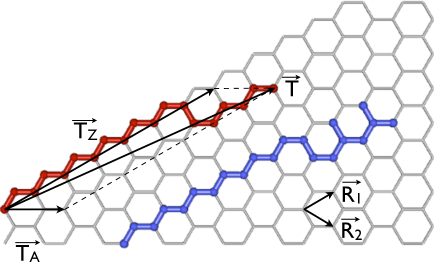
Figure 1: (Color online) Graphene lattice and the translation vector T $(n,m)=(8,1)$. The vectors T_Z and T_A are projections of T into the zigzag and armchair directions. The primitive lattice vectors R₁ and R₁ are also shown so that T= $n$R${}_{1}+m$R₂. The dark-grey (red) line shows the minimal edge; the light-grey (blue) line shows a modified edge constructed by attaching two Klein nodes to the minimal case.

Any minimal edge can be modified by adding extra edge nodes. To identify a modified edge one has just to add information on the extra nodes added to the corresponding minimal edge. As an example, Fig. 1 presents two edges associated to the translation vector ${\bf T}$ $(8,1)$. The minimal edge is marked by a red line. Another possible edge, with two additional nodes, constituting the so-called Klein defects, is marked by a blue line.

The translation vector ${\bf T}=n{\bf R}_{1}+m{\bf R}_{2}$ defining any graphene edge can be decomposed into two important directions in the honeycomb lattice (see Fig. 1), namely the armchair and zigzag: ${\bf T}={\bf T}_{A}+{\bf T}_{Z}$. Note that ${\bf T}_{Z}=(n-m){\bf R}_{1}$ and ${\bf T}_{A}=m({\bf R}_{1}+{\bf R}_{2})$. This decomposition is crucial in our analysis, since it is well-known that an armchair edge does not have $E=0$ localized states, while the zigzag termination reveals a flat edge band at Fermi energy (in the $\pi$ electron approximation) for the wavevector $k>2/3\pi$, as shown in previous nanoribbon band structure calculations fujita_1996 ; nakada . Also, it is easy to see that a minimal edge corresponding to ${\bf T}$ is a simple combination of the zigzag edge along ${\bf T}_{Z}$ and the armchair edge along ${\bf T}_{A}$.

The schematic spectrum (close to $E_{F}$) of the zigzag edge defined by the smallest ${\bf T}_{Z}={\bf R}_{1}$, i.e., the edge (1,0), is shown in the upper left panel of Fig. 2. The spectrum of a zigzag $(n-m,0)=(S,0)$ edge defined by ${\bf T}_{Z}=S{\bf R}_{1}$ is obtained by folding this spectrum $S$-times. The (2,0) case is shown explicitly in the upper right panel of Fig. 2. Both, the (1,0) and the (2,0) edge, have degeneracy 1. By repeated folding of the minimum (1,0) zigzag edge one can easily find the bandstructure and edge band degeneracies of a general $(S,0)$ edge. Any integer number $S>0$ can be written as $S=I+3M$, where $I=1,2,3$ and $M=0,1,2,...$. For $I=1$ and 2 the folded spectrum has always the Dirac point at $2/3\pi$ while for $I=3$ the Dirac point is at $k=0$, as illustrated in Fig. 2. The schematic band structures of all zigzag edges obtained from this folding are shown in Fig. 2. The degeneracies of the zero-energy band are also indicated in the lower panels ($M$ and $M+1$) close to the corresponding edge bands.

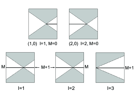
Figure 2: Schematic band structures of zigzag (1,0), (2,0) and general $(S,0)$ edges after folding the (1,0) zigzag edge band, where $S=I+3M$ as described in the text. The shaded areas represent the band continuum of states. Degeneracies of the zero-energy bands ($M$, $M+1$) are indicated in the lower panels close to the corresponding edge bands at the Fermi energy. They correspond to semi-infinite graphene sheet with only one edge. In case of a GNR with equal edges the degeneracies are doubled.

Since the armchair component does not provide any edge states, one can expect that the spectrum of a minimal-edge $(n,m)$ will be similar to the spectrum of the $(n-m,0)$ zigzag edge at least close to $E_{F}$. We have performed tight-binding calculations for a large number of different minimal-edge GNRs, and verified that the presented above folding rule holds in all the cases considered. Notice that for a graphene nanoribbon with two equal edges, the degeneracy of the flat band is twice that of the isolated edge, provided that the ribbon is wide enough to neglect interaction between the edges.

In order to construct ribbons corresponding to a particular edge ${\bf T}$, we first define the vector ${\bf H}$ as the smallest graphene lattice vector perpendicular to ${\bf T}$. The width of the ribbons studied here is spanned by a vector ${\bf W}$ given by an integer multiple of ${\bf H}$, ${\bf W}=N{\bf H}$ as it is shown in Fig. 3 for the case of 2(7,1) GNR. For a fixed ${\bf T}$, ${\bf H}$ is uniquely determined up to a global plus or minus sign; therefore, for our purposes, the ribbons with minimal edges are labeled by $N(n,m)$, where $N$ states the ribbon width, and $(n,m)$ indicates the minimal edge.

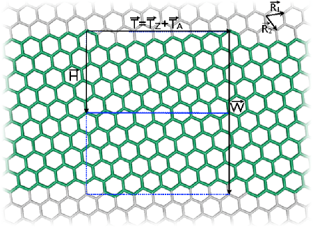
Figure 3: (Color online) Geometric structure of the 2(7,1) GNR highlighted in dark grey (green) on a graphene sheet, indicating the translation vector ${\bf T}={\bf T}_{Z}+{\bf T}_{A}$ and the width vector ${\bf W}=2{\bf H}$, where ${\bf H}$ is the smallest nanoribbon width vector belonging to the graphene lattice. ${\bf T}_{Z}=6{\bf T}(1,0)$. The unit cells spanned by T and H or W are marked.

Of course, there exist ribbons with minimal edge geometries, that may require a semi-integer $N$, such as the so-called antizigzag ribbons. As our main goal here is to study edge bands, we restrict ourselves to integer $N$, using values which yield non-interacting GNR edges.

As a particular example, the spectrum of a nanoribbon with minimal-edge 3(8,1) is presented in the left panel of Fig. 4. One can easily see that degeneracies of the flat $E=0$ bands are exactly the same as for the 20(7,0) zigzag GNR (right panel of Fig. 4). Also the gaps at $k=0$ and $\pi$ follow the folding rule to a large extent. In general, the minimal-edge $(n,m)$ GNR reveals the same zero-energy bands as the $(n-m,0)$ zigzag GNR, which in turn has the same spectrum as the $(n-m)$ times folded spectrum of the (1,0) zigzag nanoribbon of the same width.

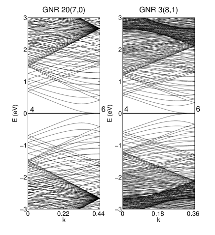
Figure 4: Energy spectra of the 20(7,0) GNR (left) and the 3(8,1) GNR (right) close to the Fermi energy. The unit cells of both GNRs contain similar number of nodes. The degeneracies of the zero-energy edge bands (4 and 6) are indicated close to extreme $k$ values.

III Modified edges

III.1 Coupling of edge defects and band splitting

Here we study a couple of modified zigzag edges. We start with the Klein defects,klein which consist of atoms with only one neighbor, as depicted in Fig. 5(a). Then we proceed with other modified edges related to the so-called cove structures, which can be constructed by adding extra atoms to the Klein-edge zigzag nanoribbon. The basic unit of such modified edges is what we call a cape. This can be built by bonding two Klein defects to one extra atom, and the resulting structure is depicted in Fig. 5(b). When extra atoms are added every two Klein defects, one gets the cove edge, shown in Fig. 5(c). We will consider modified edges where capes are more separated than in the cove edge structure, as in Fig. 5(d). Based on these examples we discuss how such modifications influence the mixing and splitting of states at $E=0$. In order to perform numerical calculations, we choose wide ribbons with equal edges. As discussed in the previous Section, if the ribbons are wide enough, the interaction between edges is reduced; and as they have equal edges, the degeneracies are obviously twice those stated in Sec. II.

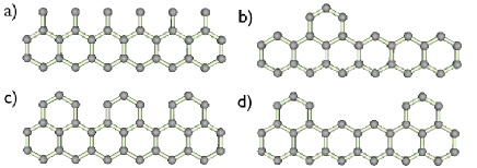
Figure 5: Geometries of several modified zigzag graphene edges. (a) Bearded zigzag edge, composed of Klein defects; (b) a cape structure on a zigzag edge, obtained by bonding one extra atom to two adjacent Klein defects; (c) a cove edge; (d) a periodic modified edge with a cape.

III.1.1 Zigzag edge with Klein defects

We consider first a simple zigzag nanoribbon modified by Klein defects. The spectrum of a zigzag nanoribbon of width 40 and minimal edge, i.e., a 40(1,0) GNR, is presented in Fig. 6(a). The two zero-energy edge bands localized at opposite edgesnakada of the GNR extend for $k>2/3\pi$. The condition to get $E=0$ requires a non-vanishing amplitude of the wavefunction in one of the two graphene sublatticeswakabayashi_2001 . For $k=\pi$ the corresponding wavefunctions are localized at the edge nodes. Opposite zigzag edges have atoms belonging to different sublattices. For $k$ closer to $2/3\pi$ the wavefunctions corresponding to these edge bands penetrate more into the inner part of the GNR; therefore, the edge states interact more for these lower $k$ values, mixing and splitting into bonding and antibonding bands.

When Klein defects are added to both sides of the GNR, the flat bands appear from $k=0$ to $2/3\pi$. In order to understand this change on the flat $E=0$ bands with respect to $k$ values, we gradually modify the coupling of the extra atoms conforming the Klein bearded edge.

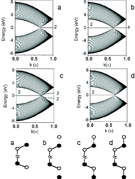
Figure 6: Evolution of the spectrum of 40(1,0) zigzag GNR (a) to the spectrum of 40(1,0) GNR with Klein nodes attached at both sides (d). In (b), two extra non-attached nodes introduce a doubly degenerate $E=0$ flat band. In (c), connecting the extra nodes with $t=0.5t_{0}$ couples and split the flat bands in the range of $k>2/3\pi$. The bottom panel illustrates how the extra nodes are attached to the upper and lower part of the unit cell of the zigzag GNR.

We first add a Klein node at each side of the GNR unit cell, but setting the hoppings equal to zero. As the on-site energies of these extra atoms are set to zero, an additional doubly degenerated zero-energy band appears, as shown in the spectrum of Fig. 6(b). The double degeneracy is due to the contribution of the two edges. Let us now switch on the hopping, setting $t=0.5t_{0}$. The resulting spectrum is shown in Fig. 6(c). The hopping connects atoms that belong to different sublattices; this allows for the interaction of the corresponding flat bands, which hybridize and split. Such splitting is more pronounced for $k=\pi$, since their localization and overlap is stronger than for any other $k$, and increases gradually from $k=2/3\pi$ to the edge of the Brillouin zone. Finally, when $t=t_{0}$, see Fig. 6d, the splitting is so strong that the bonding and antibonding bands interact from $k=2/3\pi$ to $k=\pi$ and reach the continuum of bands. We end up with the spectrum of a zigzag GNR with Klein edges, which has a zero-energy flat band for $k<2/3\pi$.

A closer inspection of the analytical TB solution for the $E=0$ band of zigzag GNR with Klein edges reveals that, contrary to the zigzag edge, the wavefunction never localizes only at the Klein nodes. The wavefunction penetrates into GNR even for $k=0$: the damping factor equals 1/2 in this case and rises up to 1 for $k=2/3\pi$.

It is noteworthy that if we modify only one edge by adding Klein nodes, the extra zero-energy band will be non-degenerate and will mix and split with only one of the edge bands in the range of $k>2/3\pi$. This mixed band is obviously localized at the edge where the Klein nodes are added.

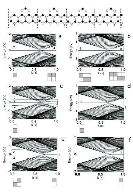
Figure 7: Evolution of the spectrum of a (4,0) zigzag GNR when extra edge nodes are added to form a single cape structure. The upper panel shows the edge of GNR where connections to extra nodes are marked by dotted lines. The four unit cells are marked by dashed lines. The steps are the following: (a) pure (4,0) GNR, (b) with two disconnected extra nodes at each side of unit cell, (c) with two extra nodes (i.e. Klein defects) connected by $t=0.2t_{0}$, (d) with two Klein nodes fully connected, (e) with another extra node connected to the Klein nodes by $t=0.2t_{0}$ forming the cape structure, and (f) with a cape structure added to the edge and all extra nodes fully connected. Diagrams illustrate the mixing and splitting of flat bands, to be explained in the text.

III.1.2 Zigzag edge modified with a cape structure

Here we consider a more complex modification of the zigzag edge. It helps to illustrate and refine in detail the presented prescription, which allows us to predict the occurrence and degeneracies of edge states for any nanoribbon. The top panel of Fig. 7 shows the construction of the cape at the upper edge only. In a similar way the cape is formed at the lower edge, but the black and open circels are reversed there.

We have considered the (4,0) zigzag GNR and a sequential addition of nodes to get the edges with a cape structure, as shown in Fig. 7. The procedure follows the next sequence. One starts from a zigzag ribbon with quadrupled unit cell. Two extra adjacent Klein nodes (open circles) are next added. Finally, the pair of Klein nodes is connected via another extra node (black circle), to form the cape structure.

The spectrum around the Fermi level of the zigzag 40(4,0) GNR is presented in Fig. 7(a). It is obtained by folding four times the spectrum of Fig. 6(a). The edge band degeneracies indicated in the Figure result from this folding. The two non-connected Klein nodes at each side of the GNR unit cell (a total of four extra nodes) yields the addition of a four-fold degenerate flat band at zero energy. The degeneracies sum up to six and eight at $k=0$ and $k=\pi$, respectively. This is shown in Fig. 7(b). We begin by connecting these extra nodes with a small hopping $t=0.2t_{0}$ and plotting the bands in Fig. 7(c). For $k>2/3\pi$ all the flat bands mix and split; they are still doubly degenerated since both edges of the GNR are equal. For $k<2/3\pi$ only two bands split and a doubly degenerate flat band survives at $E=0$. When $t=t_{0}$, see Fig. 7(d), all the split bands merge into the states continuum. The flat bands that survived at $E=0$ reveals that they are mainly localized at the extra Klein nodes and enter into GNR nodes of the same sublattice. Their spreading into the GNR is similar to that found in the flat bands of zigzag GNRs with Klein edges (see Fig. 6(d)).

To form the (4,0) GNR with a single cape structure we must add yet another extra node and connect it to the existing Klein nodes. Note that the extra node and the Klein nodes belong to different sublattices. A non-connected node adds a doubly degenerate zero-energy band to the spectrum of Fig. 7(d). When connecting this extra atom to the previous Klein nodes with $t=0.5t_{0}$, the flat bands at $k<2/3\pi$, which are due to the Klein defects, hybridize with these added bands arising from the extra connected nodes and split. This splitting is shown in Fig. 7(e). For $t=t_{0}$, as seen in Fig. 7(f). Due to the strong coupling, the bands split so much that they merge into the continuum of states. This doubly degenerate flat band at $k>2/3\pi$ appears due to the introduction of the outermost extra atoms, and as there were no localized bands at that $k$ range which could mix with them, they remain localized in the extra node, spreading into nodes belonging to the same sublattice.

This localization is confirmed by numerical calculations performed within the tight-binding model, as well as using first-principles DFT approachdft . The obtained wavefunctions are shown in the right panel of Fig. 8. Their localization in the (4,0) GNR with a single cape is different from the case of the cove edge,wakabayashi_2010 which can be considered as built from a (2,0) GNR with a cape structure (see Fig. 5c). In Ref. wakabayashi_2010, it was shown that in the case of cove edge the wavefunctions of the zero-energy bands are not localized at the outermost edge atoms, but at the neighboring nodes which belong to the other sublattice. We confirm this finding, both in the tight-binding and the DFT calculations shown in the left panel of Fig. 8 comment .

One would naively expect that the wave function should be more localized at the outermost atoms, which seems more exposed to a chemical attack. However, it is easy to check that in a cove edge, the majority of the edge atoms are not the outermost ones, but rather their nearest neighbors. The edge state is therefore localized in the atoms closest to the outermost ones, which belong to the opposite sublattice, whereas the wavefunction weight of the outermost node is zero in the tight-binding or negligible in the DFT approach. For the same reason, in a larger zigzag edge with a single cape structure such as that shown in Fig. 7, the majority of edge atoms are from the original zigzag edge, which belong to the same sublattice as the outermost atoms of the cape structures. In this case the weight in the edge state is thus in the sublattice of the majority of the zigzag edge atoms, with a nonzero value in the outermost cape node, as illustrated in the right part of Fig. 8.

III.2 Mixing and splitting diagrams

As discussed in the previous Sections, the mixing and splitting of the flat bands wavefunctions occur due to the hybridization of orbitals between neighboring nodes, which belong to different sublattices. We introduce simple diagrams that help to understand such hybridization. We can explain how such bands at $E=0$ split and their wavefunctions localize.

Each diagram is built of two rows containing square boxes where each box represents a non-degenerate band at zero energy. The upper and lower rows correspond to the upper and lower GNR edges, respectively. Empty and filled boxes represent bands that localize at different sublattices. Each extra node added to a given edge is represented by a box added to the corresponding row. The added box is empty or filled depending on the sublattice it belongs to. A pair of empty and filled boxes in a given row represents now two interacting and hybridizing bands which must split and move away from zero energy. Their corresponding pair of empty and filled boxes annihilate and disappear from the row. The remaining boxes represent the flat bands which survive such hybridization process. Their filling determines the sublattice at which they localize.

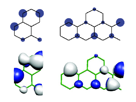
Figure 8: (Color online) Localization of the wavefunctions corresponding to the $E=0$ band at $k=\pi$ for 40(2,0) (left) and 40(4,0) (right) GNR with a cape structure at the edges. The corresponding edges are shown in Fig. 5 (c) and (d), respectively. Only an edge and a few neighboring nodes in the GNRs unit cells are shown. Upper panel: Results obtained using tight-binding method. Bottom panel: Results of first-principles calculations. The dot diameter in the upper panel reflects the TB density at the nodes. No dot means that the wavefunction is exactly zero at this node.

We describe next how the diagrams explain the mixing and splitting of the flat bands in a practical case. We consider extra nodes added to the edge of (4,0) GNR to form a ribbon with a cape structure, as shown previously in Fig. 7.

The diagram corresponding to Fig. 7(a), i.e. to the (4,0) zigzag GNR, has for $k<2/3\pi$ one filled box in the upper row (representing an $E=0$ state localized at the upper edge, on the sublattice marked by filled circles) and one empty box in the lower row (representing an $E=0$ state localized at the lower edge, on the sublattice marked by empty circles). For $k>2/3\pi$ we have two filled boxes in the upper row and two empty boxes in the lower row. We have already described the process of adding two extra Klein nodes in the previous subsection. The corresponding diagrams are shown under the bands depicted in Fig. 7(b) and (c). The two Klein nodes at each side of the GNR unit cell add two empty/filled boxes in the upper/lower rows (Fig. 7(b)). The pairs of empty/filled boxes in each row annihilate (Fig. 7(c)) and the corresponding bands split. Two boxes are only left at the Fermi energy for $k<2/3\pi$ as shown in Fig. 7(d).

The (4,0) GNR with a cape structure has an extra node connected to the existing Klein nodes at each side of the GNR. When these extra nodes are not connected, two additional $E=0$ bands appear in the spectrum. They are represented by two extra boxes added to the existing diagram: filled box in the upper row, and an empty box in the lower row. Now, for $k<2/3\pi$ the pair of filled/empty boxes in a given row annihilates, leading to the hybridization and splitting of the zero-energy bands, as shown in Fig. 7(e) and (f). For $k>2/3\pi$ the remaining two boxes do not have any partner state to hybridize, therefore they origin the states at $E=0$ which are localized in the external cape node and its sublattice. Our prescription and diagram analysis confirms the degeneracy and localization of bands as seen in the previous Subsection, but without performing any calculations.

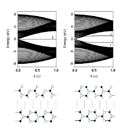
Figure 9: Spectra of armchair GNRs with Klein nodes added to the edge. Left: 40(1,1) armchair GNR with one Klein node per unit cell. Right: the same GNR but with two Klein nodes per unit cell.

III.3 Gap states away from the Fermi energy

We have already observed (see Fig. 7(d)) that in some cases the split bands do not reach the bulk continuum and for some range of $k$ they form gap states with $E\neq 0$. Similar bands occur in the bearded edges investigated in Ref. wakabayashi_2010, , where zigzag edges and Klein defects appear alternatively. nota_b Gap states with $E\neq 0$ are usually related to edges of mixed character. In this section we consider only two examples of such edges and explain their origin in more detail as an illustration of how our prescription applies to any kind of edges of mixed character.

III.3.1 Klein defects in armchair edges

Let us consider the case of an armchair ribbon with one edge modified by attaching a Klein node. The corresponding spectrum is shown in the upper left panel of Fig. 9. When both edges are modified the flat band is doubly degenerate.wakabayashi_2010 ; note2 It is noteworthy that the same flat band appears no matter whether the Klein node is disconnected or attached. Our prescription explains this fact in a simple way: such a flat band has no partner band to hybridize and split. When a second Klein node is attached (see the bottom right panel of Fig. 9), the flat bands mix and split because they belong to different sublattices. However, they do not reach the band continuum and become $E\neq 0$ gap states. When we additionally connect the previous two Klein nodes we obtain again an armchair GNR. In this case the bands split even farther and merge into the continuum; we recover the spectrum of armchair GNR.

III.3.2 Chiral edges

In this Subsection we present the results corresponding to general $(n,m)$ edges, i.e., those which are not purely armchair or zigzag, either minimal or modified. Their borders with Klein defects and the corresponding spectra can be explained by the folding rule and diagrams presented above.

As example, we investigate a 3(8,1) GNR with a minimal edge and two different modifications. Studying different edges for a given translation vector ${\bf T}$ is important, since different edge modifications are required sometimes to form junctions between graphene edges, as it happens when constructing junctions between carbon nanotubes. Such studies suggest whether localized or resonance interface states appear at the junctions and even allow to estimate their energiessantos .

Figure 10: Spectra of 3(8,1) GNR close to the Fermi energy with different edge terminations, ranging from the minimal edge (a) to the modified edge with one Klein node, marked as A, added (b-c) or two Klein nodes A and B attached (d). In (b) $t=0.1t_{0}$, while in (c) and (d) $t=t_{0}$. The top panels show the minimal and modified edges.

The top panel of Fig. 10 shows the different edges investigated: minimal (left) and modified (right) by attaching one, A, or two, A and B, Klein nodes. The spectrum of the GNR with minimal edges close to $E_{F}$ is shown in Fig. 10(a). Note that it is the same spectrum as in Fig. 4(right). The degeneracy of the $E=0$ band results from the folding rules corresponding to the (7,0) GNR. When an extra non-connected node (marked as A in the Figure) is added at each side of the GNR unit cell, a doubly degenerated $E=0$ band appears in the spectrum. Thus, the degeneracies increase to six and eight for $k<2/3\pi$ and $k>2/3\pi$, respectively. When we connect this extra node by $t=0.1t_{0}$, two flat bands hybridize and split, see Fig. 10(b). The hybridization and splitting can be explained by the attached diagrams. For $t=t_{0}$ the split bands merge into the ribbon continuum of states and disappear from the gap region; the spectrum and the corresponding diagrams are shown in Fig. 10(c). If the other Klein node marked B is added to this edge, first as a non-connected node, the degeneracy of the $E=0$ ribbon band increases by two. If the connection of the atom B is turned on, the bands mix and split. Fig. 10(d) shows the bands for $t=t_{0}$. All the boxes in the diagram corresponding to $k<2/3\pi$ annihilate. Only a doubly degenerate zero-energy band survives for $k>2/3\pi$. In the corresponding diagram two pairs of empty and filled boxes annihilate, leaving only one box in each row that corresponds to a doubly degenerate band at zero energy. The attached diagrams also indicate that the flat bands in both cases (c) and (d) localize in the sublattices corresponding to the zigzag edges. Our numerical calculations fully confirm again these predictions.

A comment is required to explain why the addition of the second Klein node B yields weaker splitting of the flat bands than in the case where only a node A is attached. A closer inspection of the two wavefunctions localized at one edge at $k=0$ in Fig. 10a reveals that one of them is nearest to a step in the edge, see upper panel. Such step-localized wavefunction is thus nearer to the Klein defects. The second wavefunction at B localizes away from the step. Attaching the first Klein node A yields a strong hybridization with the step-localized wavefunction. The wavefunction of the second Klein node B must hybridize with the remaining function, which localizes away from the Klein node. This explains why the mixing of B is weaker and its splitting smaller.

IV Summary

We have presented a simple prescription to predict, without performing any calculations, the existence of zero-energy bands in graphene nanoribbons and graphene edges of arbitrary shape. Our prescription is based on two observations: (a) any edge can be created from a minimal edge by adding extra nodes, (b) the zero-energy spectra of graphene minimal edges are uniquely defined by the edge band structure of its zigzag $(n,0)$ component, which in turn is obtained by folding $n$ times the spectrum of the zigzag (1,0) edge. Extra but disconnected nodes provide zero-energy states which, after connecting them to the graphene edge, may hybridize with the existing flat bands and split. The splitting occurs only when the extra node belongs to a different sublattice as that where the edge zero-energy bands are localized. We have introduced simple rules and diagrams allowing to precisely determine not only the existence of the flat bands, but also their degeneracies and localization of their wavefunctions on the graphene sublattices. The folding rules allow also to estimate the energy gaps which open in certain regions of $k$. Our prescription and diagrams hold for graphene edges and nanoribbons with arbitrary geomeries. However, one has to remember that for extremely narrow ribbons the interaction between the GNR edges may lead to the edge bands splitting and the loss of their flatness.

We have considered a number of GNRs with different edges, some of them with attached Klein nodes or cape structures. They are also important in the study of graphene-based complex systems, since connecting different portions of graphene requires sometimes the modification of their edges.

Finally, we have shown that our prescription predicts the localization properties of edge states. We have studied a couple of cases by performing tight-binding and first-principles DFT calculations. The correspondence between the ab-initio and the tight-binding results back our prescriptions, with the caveat that within the DFT approach the edge bands are no longer exactly flat and with zero-energy. Our method can be widely used to foresee the existence of edge states and flat bands in any graphene edges and ribbons.

V Acknowledgments

We acknowledge financial support from Basque Departamento de Educación and the UPV/EHU (Grant No. IT-366-07), the Spanish Ministerio de Innovación, Ciencia y Tecnología (Grants No. FIS2007-66711-C02-02 and FIS2009-08744) and the ETORTEK research program funded by the Basque Departamento de Industria and the Diputación Foral de Guipúzcoa. W.J. thanks Donostia International Physics Center, and A.A. and L.C. thank Nicolaus Copernicus University in Toruń for hospitality.

References

- (1) A. H. Castro Neto, F. Guinea, N. M. R. Peres, K. S. Novoselov, and A. K. Geim, Rev. Mod. Phys. 81, 109 (2009).
- (2) Y. Zhang, Y.-W. Tan, H. L. Stormer, and P. Kim, Nature (London) 438, 201 (2006).
- (3) C. L. Kane, and E. J. Mele, Phys. Rev. Lett. 95, 226801 (2005)
- (4) Y. W. Son, M. L. Cohen, and S. G. Louie, Nature (London) 444, 347 (2006).
- (5) M. Fujita, K. Wakabayashi, K. Nakada, and K. Kusakabe, J. Phys. Soc. Jpn. 65, 1920 (1996).
- (6) K. Nakada, M. Fujita, G. Dresselhaus, and M.S. Dresselhaus, Phys. Rev. B 54, 17954 (1996).
- (7) K. S. Novoselov, A. K. Geim, S. V. Morozov, D. Jiang, Y. Zhang, S. V. Dubonos, I. V. Grigorieva, and A. A. Firsov, Science 306, 5296 (2004).
- (8) L. Brey, and H. A. Fertig, Phys. Rev. B 73, 235411 (2006).
- (9) H. Zheng, Z. F. Wang, T. Luo, Q. W. Shi, and J. Chen, Phys. Rev. B 75, 165414 (2007).
- (10) Y. W. Son, M. L. Cohen, and S. G. Louie, Phys. Rev. Lett. 97, 216803 (2006).
- (11) A. Cresti and S. Roche, Phys. Rev. B 79, 233404 (2009).
- (12) Y. Niimi, T. Matsui, H. Kambara, K. Tagami, M. Tsukada, and Hiroshi Fukuyama, Phys. Rev. B 73, 085421 (2006).
- (13) Y. Kobayashi, K.-I. Fukui, T. Enoki, and K. Kusakabe, Phys. Rev. B 73, 125415 (2006).
- (14) Z. Liu, K. Suenaga, P. J. F. Harris, and S. Iijima, Phys. Rev. Lett. 102, 015501 (2009).
- (15) K. Suenaga and M. Koshino, Nature (London) 468, 1088 (2010).
- (16) K. Wakabayashi, Phys. Rev. B 64, 125428 (2001).
- (17) A. R. Akhmerov and C. W. Beenakker, Phys. Rev. B 77, 085423 (2008). .
- (18) D. J. Klein, Chem. Phys. Lett. 217, 261 (1994).
- (19) K. Wakabayashi, S. Okada, R. Tomita, S. Fujimoto, and Y. Natsume, J. Phys. Soc. Jpn. 79, 034706 (2010).
- (20) For a width of 10 zigzag unit cells, we use SIESTA method to solve the Kohn-Sham equations using for the exchange-correlation functional the generalized gradient approach of Perdew-Burke-Ernzerhof. J. M. Soler, E. Artacho, J. D. Gale, A. García, J. Junquera, P. Ordejón, and D. Sánchez-Portal, J. Physics: Condensed Matter 14, 2745 (2002); J. P. Perdew, K. Burke and M. Ernzerhof, Phys. Rev. Lett. 77, 3865 (1996). The number of K points were converged and the atoms were relaxed until the forces were smaller than 0.02 eV/Å.
- (21) The energy bands at E=0 of TB method split in DFT calculations. The small splitting arises from the spin polarization at the edges [Ref. magnetic, ; A. Mañanes, F. Duque, A. Ayuela, M. J. López, and J. A. Alonso, Phys. Rev. B 78, 035432 (2008)], but it does not change our main TB conclusions. For the cape studies, the inclusion of spin polarization removes the double degeneracy of E=0 band, but they remain close to the Fermi energy.
- (22) When both Klein nodes belong to the same sublattice the degeneracy is exact for all , otherwise the bands will split for narrow ribbons.
- (23) H. Santos, A. Ayuela, W. Jaskolski, M. Pelc, and L. Chico, Phys. Rev. B. 80, 035436 (2009).
- (24) W. Yao, S. A. Yang, and Q. Niu, Phys. Rev. Lett. 102, 096801 (2009).
- (25) D. Gunlycke, D. A. Areshkin, and C. T. White, Appl. Phys. Lett 90, 142104 (2007).
- (26) The band structure of these ribbons with bearded edges can be easily explained with our prescription. It is sufficient to consider a (2,0) GNR with only one Klein defect added at each side of the GNR unit cell.