The Cosmological Constant as a Ghost of Inflaton

Abstract

The cosmological constant (term) is the simplest way, presently known, to illustrate the accelerating expansion of the universe. However, because of/despite its simple appearance, there is much confusion surrounding its essence. Theorists have been asking questions for years: Is there a mechanism to explain this term? Is it really a constant or a variable? Moreover, it seems that we have created a huge gulf separating the theories of inflation and accelerating expansion. Can we eliminate such an uncomfortable discontinuity?

In this paper, we will journey to see the growth of the universe from the very beginning of inflation. To simplify our discussion, we will briefly “turn off” the effects of real and dark matter and shall use inflaton (a classical scalar field) dynamics with a time-varying inflaton potential $V\left(\phi,t\right)$ as the screen to watch this process. Relying on these conditions, we propose a non-traditional method of obtaining the solution of scale factor $\mathrm{R}\left(t\right)$, which is only dependent on $\dot{\phi}^{2}$, and discover that the term $\nicefrac{{\ddot{\mathrm{R}}\left(t\right)}}{{\mathrm{R}\left(t\right)}}$ will be a constant after kinetic inflaton $\dot{\phi}$ is at rest. This result can be regarded as the effective cosmological constant phenomenally. Moreover, we will also “rebuild” $V\left(\phi,t\right)$, realize its evolutionary process and then, according to the relationship between $V\left(\phi,t\right)$ and $\dot{\phi}^{2}$, it will be possible to smoothly describe the whole evolution of the universe from the epoch of inflation. Therefore, the implications of our findings will mean that the gulf between theories will disappear. Lastly, we will also see how the formula could provide a framework for solving the old and new cosmological constant problems as well as much more besides.

I introduction

According to observational data key-1 ; key-2 ; key-3 ; key-4 ; key-5 ; key-6 , the major components required to build the universe as we see it today are 73% dark energy, 22% dark matter, 5% observable matter and about 0.008% radiation. "Dark energy" is introduced theoretically to explain the accelerating expansion of the universe and, as the word “dark” implies, only few of its properties are known. Firstly, for example, according to the 1st Friedmann equation without the cosmological constant

$$\frac{\ddot{\mathrm{R}}}{\mathrm{R}}=-\frac{4\pi G}{3c^{2}}\left(\varepsilon+3p\right),$$ (1)

the equation of state $\omega\equiv\nicefrac{{p}}{{\varepsilon}}<\nicefrac{{-1}}{{3}}$ (where $\varepsilon$ is the energy density and $p$ is the pressure) should be satisfied in order to make the "anti-gravity" $\ddot{\mathrm{R}}>0$ become possible on the large scales of the universe; secondly, the repulsive properties of dark energy require its distribution to be highly homogenous and isotropic; thirdly, observations show its density to be roughly $10^{4}\,\nicefrac{\mathrm{eV}}{\mathrm{cm^{3}}}$ key-7 ; and finally there is still no evidence to suggest that it interacts with matter through any of the fundamental forces other than gravity. Up to the present moment, many dark energy models key-35 ; key-36 ; key-37 ; key-38 ; key-39 ; key-40 ; key-41 have been proposed and we should not, of course, forget the simplest one which was introduced by Einstein in 1917 key-8 :

$$R_{\mu\nu}-\lambda g_{\mu\nu}=-\frac{8\pi G}{c^{4}}\left(T_{\mu\nu}-\frac{1}{2}g_{\mu\nu}T\right).$$ (2)

Here, the term $\lambda$ is the one that Einstein famously described as "the biggest blunder of (his) life." Marvelously, however, the cosmological constant has gone on to become a charming topic of cosmology and fundamental physics today key-10 ; key-42 ; key-43 ; key-44 ; key-45 ; key-46 . Indeed, the mere history of the topic informs us of how strange of the cosmological constant is. Based on his belief in Mach’s principle, in 1917 Einstein inserted the cosmological term $\lambda$ into (2) so as to keep the universe static. Soon, de Sitter key-9 proposed another static solution controlled only by $\lambda$,

$$ds^{2}=\frac{1}{\cosh^{2}\left(\mathcal{H}r\right)}\left\{c^{2}dt^{2}-dr^{2}-H^{-2}\sinh^{2}\left(\mathcal{H}r\right)\left[d\theta^{2}+\sin^{2}\theta d\varphi^{2}\right]\right\},$$ (3)

where the corresponding conditions are $\varepsilon=p=0$ and $\lambda=\frac{3}{\mathrm{R}^{2}}=3\mathcal{H}^{2}$ ($\mathrm{R}$ is the radius of a 3-sphere universe). Several years later, Weyl pointed out that a test body on de Sitter’s metric would display a redshift because the term $\Gamma_{tt}^{r}=-c^{2}\mathcal{H}\tanh\left(\mathcal{H}r\right)\neq 0$ would give a redshift $z\simeq\mathcal{H}r\ll 1$ key-10 . Therefore, even though Hubble’s discovery key-11 was not yet published, Einstein mailed Wely in 1923 to give his reaction: “If there is no quasi-static world, then away with the cosmological term!” key-10

However, the cosmological term can not be abandoned so easily. According to quantum field theory, anything that contributes to the energy density of vacuum must act exactly like a cosmological constant. To repeat Weinberg’s elegant report key-10 , the vacuum energy-momentum tensor must take the form

$$\left\langle T_{\mu\nu}\right\rangle_{\mathrm{vac}}=\left\langle\varepsilon_{\mathrm{vac}}\right\rangle g_{\mu\nu}$$ (4)

to obey the Lorentz invariance (where we set $g_{00}=c^{2}$) and the 2nd Fridemann equation in flat spacetime

$$H^{2}=\left(\frac{\mathrm{\dot{R}}}{\mathrm{R}}\right)^{2}=\frac{8\pi G}{3c^{2}}\left\langle\varepsilon_{\mathrm{tot}}\right\rangle+\frac{\lambda c^{2}}{3},$$ (5)

where the total density can be separated into the ordinary part and the vacuum part as

$$\left\langle\varepsilon_{\mathrm{tot}}\right\rangle=\left\langle\varepsilon_{\mathrm{ord}}\right\rangle+\left\langle\varepsilon_{\mathrm{vac}}\right\rangle.$$ (6)

From this we can see that the effective cosmological constant in density formation would be

$$\varepsilon_{\mathrm{eff}}=\frac{\lambda c^{4}}{8\pi G}+\left\langle\varepsilon_{\mathrm{vac}}\right\rangle.$$ (7)

Now let us introduce the critical density

$$\varepsilon_{\mathrm{crit}}\equiv\frac{3c^{2}H_{0}^{2}}{8\pi G}\simeq 5.16\times 10^{3}\,\nicefrac{\mathrm{eV}}{\mathrm{cm^{3}}},$$ (8)

with the Hubble constant at its present day value of $H_{0}\approx 70\,\nicefrac{\mathrm{\nicefrac{\mathrm{km}}{\mathrm{s}}}}{\mathrm{Mpc}}$. This leaves a value for the effective density as

$$\left|\varepsilon_{\mathrm{eff}}\right|\simeq\varepsilon_{\mathrm{crit}}\times 73\%\simeq 3.76\times 10^{3}\,\nicefrac{\mathrm{eV}}{\mathrm{cm^{3}}}.$$ (9)

In addition, the vacuum density can be calculated by summing the zero-point energies of all normal modes $k$ of some field of mass $m$ up to a wave cutoff $\Lambda_{\mathrm{cut}}\gg\nicefrac{{mc}}{{\hbar}}$, as

$$\left\langle\varepsilon_{\mathrm{vac}}\right\rangle=\frac{1}{\left(2\pi\right)^{3}}\int_{0}^{\Lambda_{\mathrm{cut}}}\frac{\hbar}{2}\sqrt{k^{2}c^{2}+\frac{m^{2}c^{4}}{\hbar^{2}}}\cdot 4\pi k^{2}dk\simeq\frac{\hbar c\Lambda_{\mathrm{cut}}^{4}}{16\pi^{2}}.$$ (10)

Assuming that the smallest limit of general relativity is the Planck scale, we can take $\Lambda_{\mathrm{cut}}=\pi\sqrt{\nicefrac{{c^{3}}}{{\hbar G}}}$ into (10) to get

$$\left\langle\varepsilon_{\mathrm{vac}}\right\rangle\simeq\frac{\pi^{3}c^{7}}{16\hbar G^{2}}\simeq 5.60\times 10^{126}\,\nicefrac{\mathrm{eV}}{\mathrm{cm^{3}}}.$$ (11)

This is much more huge than the effective density as witnessed in reality. For the real world in which we live, we need Einstein’s cosmological term in order to cancel out the vacuum density of $\left|\left\langle\varepsilon_{\mathrm{vac}}\right\rangle+\nicefrac{{\lambda c^{4}}}{{8\pi G}}\right|$ to more than 123 decimal places. It is the famous "old problem" of the cosmological constant. On the other hand, the "new problem" has arisen key-1 ; key-2 because modern observations give us the very small but nonzero value of (9).

Further, as outlined in the abstract, there is a large gulf that separates certain theories. On one side is the theory of the inflationary universe that deals with the growing scale factor before $10^{-36}\,\mathrm{s}$ in cosmic time; on the other, is the theory of dark energy that describes an accelerating expansion universe at about the range of $z<2$. Of course, this represents a massive difference in cosmic time. Nevertheless, despite the discrepancy, we still wish to have a complete picture of our universe. Following this idea, we shall try to use inflationary theory as the framework for our discussion in this paper.

And now to an overview of our journey: In Section II, I will give a brief review of inflationary theory - the elegant explanation that gives us many beautiful solutions to the problems of the big bang theory. Before discussing our new proposal, it is most instructive to touch upon this topic. In Section III, I will introduce classical scalar field (inflaton) dynamics to an universe with a time-varying inflaton potential in order to find a new solution for the scale factor. In Section IV, some results of toy models will be presented to provide a clear image of the proposal and in the final section I will give a full discussion of the new proposal and try to answer the problems which have been mentioned above.

An extraneous but important point should be included here: I would like to dedicate this work to my sweet daughter CoCo, a lovely cat who was smart, charming and kind. She gave me much joy, support and inspiration and I wish to thank her for accompanying me during the past 11 years, especially through the nights when I was working and studying. During these times, if I couldn’t sleep, she didn’t sleep and it is thanks to her that I was reminded to recheck my solutions once again, searching for the important details that I had previously missed. This was her last gift before she left and it’s very sad for me: she passed away on Dec. 21, 2010.

II review of the inflationary universe theory

Motivation

After the day when Lemaître proposed what would later become known as the Hot Big Bang theory key-12 , cosmology transformed into a famous and precise discipline of physics. Finally, we were able to explore a reasonable picture of the universe without resorting to romantic and religious concepts and, consequently, puzzles like the origin of matter, the age of the universe and other complicated problems can be solved in the present day. Progress was further complimented when Gamow et al. key-13 ; key-14 ; key-15 predicted the remnant temperature that we now call cosmic microwave background radiation (CMBR) and thereby underlined Lemaître’s theory as a compelling explanation for the emergence of our universe. Regardless, even though we have achieved so much, many unsolved problems remain. The following is a list of difficulties that arose from the hot big bang theory and thus brought about the inflationary theory key-16 :

1. The homogenous and isotropic problem: according to observations, the universe is homogenous and isotropic in large scales. What is the reason for this?

2. The horizon problem: considering the initial length and the causal length close to the era of the Planck scale, we find a huge value for the ratio:

   $$\frac{l_{\mathrm{initial}}}{l_{\mathrm{causal}}}=\frac{\frac{ct_{\mathrm{now}}}{\mathrm{R}_{\mathrm{now}}}\mathrm{R}_{\mathrm{Planck}}}{ct_{\mathrm{Planck}}}\simeq 10^{28}.$$ (12)

   This is dependent on the scale-time-temperature relation

   $$\mathrm{R}\left(t\right)\varpropto\sqrt{t}\varpropto T^{-1}\left(t\right).$$ (13)

   (12) tells us that the region of CMBR that we see today is much bigger than the horizon at the last scattering.

3. The flatness problem: according to the 2nd Fridemann equation, but with an arbitrary curvature parameter $\mathrm{K}$, yields $\Omega\left(t\right)-1=\nicefrac{{\mathrm{K}}}{{\left(H\mathrm{R}\right)^{2}}}$. If we suppose the expansion of the universe is uniform , we find

   $$\frac{\Omega\left(t_{\mathrm{Planck}}\right)-1}{\Omega\left(t_{\mathrm{now}}\right)-1}\simeq 10^{-56}.$$ (14)

   This shows that the universe should be flat $\left(\mathrm{K}\approx 0\right)$ during its very early stage.

4. The initial perturbation problem: perturbation must be $\frac{\delta\varepsilon}{\varepsilon}\sim 10^{-5}$ on galactic scales to explain the large-scale structure of the universe.

5. The magnetic-monopole problem: the Grand Unified Theory (GUT) informs that lots of magnetic monopoles must have been created in the extreme heat of the early universe key-17 ; key-18 . However, we are yet to find any in the present day.

6. The total mass problem: the total mass of the observable part of the universe is $\sim 10^{60}\,\mathrm{M_{Planck}}$.

7. The total entropy problem: the total entropy we observe today is greater than $10^{87}$.

Inflation as scalar field dynamics

It is helpful now to mention a brief early history of inflationary theory. In 1974, Linde was the first to realize that the energy density of a scalar field plays the role of the vacuum energy/cosmological constant key-19 . Then, in 1979 - 1980, Starobinsky wrote the first semi-realistic model of an inflationary type key-20 . Meanwhile, at the end of the 1970s, Guth investigated the magnetic-monopole problem and found that a positive-energy false vacuum would generate an exponential expansion of space key-22 . The idea which he proposed is the model we call "old inflation" today. Unfortunately, it is afflicted by a certain problem: the probability of bubble formation would cause the universe either to be extremely inhomogeneous by way of an inflation period that was too short or to contain a long period of inflation and a separate open universe with a vanishingly small cosmological parameter $\Omega$ key-23 ; key-24 ; key-25 . Soon, therefore, a theory called "new inflation" was proposed key-26 ; key-27 . It suggested a scenario whereby the inflaton field $\phi$ should slowly roll down to the minimum of its effective potential. During slow-roll inflation, energy is released homogeneously into the whole of space and density perturbations are inversely proportional to $\dot{\phi}$ key-28 ; key-29 ; key-30 ; key-31 ; key-32 ; key-33 .

Following the brief but incomplete review above, we will now turn our attention to the construction of basic inflationary theory. Consider the action of our universe without the cosmological constant in Planck units, $c=G=\hbar=1$,

$$S_{\mathrm{u}}=\frac{1}{16\pi}\int d^{4}x\sqrt{-g}R+\int d^{4}x\sqrt{-g}\mathcal{L}_{\mathrm{m}},$$ (15)

where $R$ is Ricci scalar and $g$ is the determinate of a spacetime metric tensor. Due to the fact that inflation began before the GUT phase transition, we could say that the Lagrangian of matter was made by a dimensionless scalar field $\phi\left(x^{\mu}\right)$,

$$\mathcal{L}_{\mathrm{m}}\left(\phi,\partial_{\mu}\phi,x^{\mu}\right)=\frac{1}{2}g^{\mu\nu}\partial_{\mu}\phi\partial_{\nu}\phi-V\left(\phi,x^{\mu}\right).$$ (16)

When we vary (15) to $g_{\mu\nu}$ by the variation principle, we get the Einstein field equation

$$R_{\mu\nu}-\frac{1}{2}Rg_{\mu\nu}=-16\pi\left(\frac{\delta\mathcal{L}_{\mathrm{m}}}{\delta g^{\mu\nu}}-\frac{1}{2}g_{\mu\nu}\mathcal{L}_{\mathrm{m}}\right).$$ (17)

Look at the two equations (16) and (17). There are two keys to these equations that would enable us to investigate the universe: one is to give the structure of spacetime, i.e. the metric tensor “$g_{\mu\nu}$”; the other is to suggest a model of the matter field, i.e. the potential term “$V\left(\phi,x^{\mu}\right)$”. However, (17) tells us that the situation is too complex as $g_{\mu\nu}$ and $\phi$ vigorously interact with each other. To simplify, let us consider the formula in the bracket of (17): the energy-momentum tensor. Another formation in scalar field is

$$T_{\mu\nu}=\partial_{\mu}\phi\partial_{\nu}\phi-g_{\mu\nu}\left[\frac{1}{2}g^{\alpha\beta}\partial_{\alpha}\phi\partial_{\beta}\phi-V\left(\phi,x^{\mu}\right)\right].$$ (18)

According to observations, the spacetime metric tensor should be off-diagonal as much as possible. For this reason, we want $T_{\mu\nu}$ to approach the off-diagonal as well. When we attempt to separate the scalar field into two parts

$$\phi\left(t,x^{i}\right)=\phi\left(t\right)+\delta\phi\left(t,x^{i}\right),$$ (19)

we find that the amplitude of $\delta\phi\left(t,x^{i}\right)$ must be small enough to make the tensors adhere to the off-diagonals that we desire.

In passing through the above discussion, we become confident that $\phi\left(t\right)$ has a major role in affecting spacetime geometry. Therefore, the line element of the Friedmann–Lemaître–Robertson–Walker (FLRW) spacetime can be introduced here as the spacetime background

$$ds^{2}=dt^{2}-\mathrm{R}^{2}\left(t\right)\left[\frac{dr^{2}}{1-\mathrm{K}r^{2}}+r^{2}d\theta^{2}+r^{2}\sin^{2}\theta d\varphi^{2}\right],$$ (20)

where $\mathrm{R}\left(t\right)$ is the scale factor and $\mathrm{K}$ is the curvature parameter. Now taking (20) into (17) with the time dependent scalar field $\phi\left(t\right)$ and making the general consideration that the potential function of (16) is only dependent on $\phi$, we obtain the Fridemann equations corresponding to the scalar field:

$$\mathrm{\frac{\ddot{R}}{R}}=-\frac{8\pi}{3}\left(\dot{\phi}^{2}-V\left(\phi\right)\right),$$ (21)

$$\left(\mathrm{\frac{\dot{R}}{R}}\right)^{2}=\frac{8\pi}{3}\left(\frac{1}{2}\dot{\phi}^{2}+V\left(\phi\right)\right)-\frac{\mathrm{K}}{\mathrm{R^{2}}}.$$ (22)

Furthermore, from the fact that energy-momentum conservation requires

$$D_{\mu}T^{\mu\nu}=0,$$ (23)

where the operator $D_{\mu}$ is the covariant derivative, we obtain the scalar field equation

$$\ddot{\phi}+3\left(\mathrm{\frac{\dot{R}}{R}}\right)\dot{\phi}+\frac{dV\left(\phi\right)}{d\phi}=0$$ (24)

by taking (18) into (23).

To find the solution for the scale factor during inflation, two conditions should be noted:

1. $\dot{\phi}^{2}\ll V\left(\phi\right)$ initially makes $\ddot{\mathrm{R}}\gg 0$.

2. To avoid the bubble-formation problem, the slow-roll scenario requires $\ddot{\phi}\approx 0$ during the period of inflation.

Given the above two conditions and neglecting the curvature term $\nicefrac{{\mathrm{K}}}{{\mathrm{R^{2}}}}$ in (22) (actually, even if we keep this term to begin with, the initial stages of inflation will soon render it obsolete), potential models for inflation must satisfy the following:

1. By calculating the approximation of $\nicefrac{{-\dot{H}}}{{H^{2}}}$, we have two slow-roll parameters as defined by Liddle and Lyth key-34

   $$\epsilon\left(\phi\right)\equiv-\frac{\dot{H}}{H^{2}}\simeq\frac{1}{16\pi}\left(\frac{V^{{}^{\prime}}\left(\phi\right)}{V\left(\phi\right)}\right)^{2}\ll 1,$$ (25)

   $$\eta\left(\phi\right)\equiv\epsilon\left(\phi\right)-\frac{\ddot{\phi}}{H\dot{\phi}}\simeq\frac{1}{8\pi}\frac{V^{{}^{\prime\prime}}\left(\phi\right)}{V\left(\phi\right)}\ll 1.$$ (26)

2. According to the horizon problem, (12) and (13) tell us $\nicefrac{{\mathrm{R}_{\mathrm{now}}}}{{\mathrm{R}_{\mathrm{Planck}}}}\simeq 10^{28}\approx e^{65}$. Therefore, the e-folding number $N$ should be

   $$N\equiv\ln\frac{\mathrm{R}\left(t_{e}\right)}{\mathrm{R}\left(t_{i}\right)}\simeq-8\pi\int_{\phi_{i}}^{\phi_{e}}\left(\frac{V\left(\phi\right)}{V^{{}^{\prime}}\left(\phi\right)}\right)d\phi\gtrsim 60-70,$$ (27)

   where the suffix $i$ means the beginning of inflation and the suffix $e$ means the end of inflation.

III the ghost of inflaton

Generally, people introduce models of $V\left(\phi\right)$ for the inflation corresponding to the above discussion and, through this method, much success can be achieved. However, the setting of $\ddot{\phi}\approx 0$ during this inflation means that contributions to the damping term $-3H\dot{\phi}$ are received from the potential energy difference alone and in entirety. The setting also means that the contribution of $\ddot{\phi}$ to the damping term is prevented, and the energy exchange between the potential and kinetic terms is also turned off. Therefore, the method not only disqualifies us from obtaining a solution for the scale factor after inflation (because the scenario is specific to our universe during inflation), but also limits study to a special case for the three cosmic field equations ((21), (22) and (24)). In my opinion, even if we only have an interest in our universe, we do not need to concern ourselves with the assumption $\ddot{\phi}\approx 0$ during inflation, providing that we already know the proper inflaton models. Therefore, let us try to consider another assumption: First, we allow that the potential term of the Lagrangian (16) is time-varied as $V\left(\phi,t\right)$. Then, we can easily obtain the new cosmic field equations

$$\mathrm{\frac{\ddot{R}}{R}}=-\frac{8\pi}{3}\left(\dot{\phi}^{2}-V\left(\phi,t\right)\right),$$ (28)

$$\left(\mathrm{\frac{\dot{R}}{R}}\right)^{2}=\frac{8\pi}{3}\left(\frac{1}{2}\dot{\phi}^{2}+V\left(\phi,t\right)\right)-\frac{\mathrm{K}}{\mathrm{R^{2}}},$$ (29)

$$\ddot{\phi}\dot{\phi}+3\left(\mathrm{\frac{\dot{R}}{R}}\right)\dot{\phi}^{2}+\frac{dV\left(\phi,t\right)}{dt}=0$$ (30)

by calculating (17) and (23) with the FLRW spacetime background (20). Consequently, the equation

$$-3H\dot{\phi}^{2}=\frac{d}{dt}\left(\frac{1}{2}\dot{\phi}^{2}+V\left(\phi,t\right)\right)$$ (31)

gained from (30) is the screen for our journey, whereupon we can obtain the scale factor solution

$$\mathrm{R}\left(t\right)=\mathrm{R}\left(t_{i}\right)\exp\left[\int_{t_{i}}^{t}\left(H\left(t_{i}\right)-4\pi\int_{t_{i}}^{T}\dot{\phi}^{2}d\tau\right)dT\right]$$ (32)

by taking (29) (neglecting the curvature term $\nicefrac{{\mathrm{K}}}{{\mathrm{R^{2}}}}$) into (31). $t_{i}$ denotes the cosmic time when inflation was beginning; $t$ is an arbitrary cosmic time after $t_{i}$; $H\left(t_{i}\right)$ is a constant that needs to be determinate, called the initial Hubble parameter (IHP); and $\dot{\phi}^{2}$ is the kinetic energy term of inflaton with a value that is never negative. Of course, $H\left(t\right)=0$ is another trivial solution of (31) which does not require our concern. Next, taking the first and second derivative of $\mathrm{R}\left(t\right)$, we have

$$\left(\frac{\mathrm{\dot{R}}\left(t\right)}{\mathrm{R}\left(t\right)}\right)^{2}=\left[H\left(t_{i}\right)-4\pi\int_{t_{i}}^{t}\dot{\phi}^{2}d\tau\right]^{2},$$ (33)

$$\frac{\ddot{\mathrm{R}}\left(t\right)}{\mathrm{R}\left(t\right)}=\left[H\left(t_{i}\right)-4\pi\int_{t_{i}}^{t}\dot{\phi}^{2}d\tau\right]^{2}-4\pi\dot{\phi}^{2}\left(t\right).$$ (34)

Now, by incorporating (34) into (28), we can rebuild the time-dependent potential as

$$V\left(t\right)=\frac{3}{8\pi}\left[H\left(t_{i}\right)-4\pi\int_{t_{i}}^{t}\dot{\phi}^{2}d\tau\right]^{2}-\frac{1}{2}\dot{\phi}^{2}\left(t\right).$$ (35)

Thus, we can define the Hubble-$\lambda$-function that appears in (32), (33), (34) and (35) as

$$H_{\lambda}\left(t\right)=H\left(t_{i}\right)-4\pi\int_{t_{i}}^{t}\dot{\phi}^{2}d\tau.$$ (36)

To observe (36), the integral should be

$$\int_{t_{i}}^{t>t_{r}}\dot{\phi}^{2}d\tau=\int_{t_{i}}^{t_{r}}\dot{\phi}^{2}d\tau+\int_{t_{r}}^{t>t_{r}}\dot{\phi}^{2}d\tau=\int_{t_{i}}^{t_{r}}\dot{\phi}^{2}d\tau$$ (37)

if $\dot{\phi}$ is at rest after time $t_{r}$: i.e. $\dot{\phi}\left(t\geq t_{r}\right)=0$. Therefore, $\left(\nicefrac{{\dot{\mathrm{R}}}}{{\mathrm{R}}}\right)_{t\geq t_{r}}^{2}$ and $\left(\nicefrac{{\ddot{\mathrm{R}}}}{{\mathrm{R}}}\right)_{t\geq t_{r}}$ are non-negative constants. Comparing the 2nd Friedmann equation which is only dependent on the cosmological constant,

$$\left(\mathrm{\frac{\dot{R}\left(t\right)}{R\left(t\right)}}\right)^{2}=\frac{\Lambda}{3},$$ (38)

with (33), we come to

$$\Lambda=3H_{\lambda}^{2}\left(t\geq t_{r}\right)=3\left[H\left(t_{i}\right)-4\pi\int_{t_{i}}^{t_{r}}\dot{\phi}^{2}d\tau\right]^{2}.$$ (39)

Moreover, reviewing the earlier discussion of (7), we can treat

$$\left\langle\varepsilon_{\mathrm{vac}}\right\rangle=\frac{3H^{2}\left(t_{i}\right)}{8\pi}$$ (40)

as the vacuum energy density. Then the term for Einstein’s cosmological term would be

$$\lambda=-24\pi H\left(t_{i}\right)\int_{t_{i}}^{t_{r}}\dot{\phi}^{2}d\tau+48\pi^{2}\left(\int_{t_{i}}^{t_{r}}\dot{\phi}^{2}d\tau\right)^{2}.$$ (41)

Therefore, (39) is the effective cosmological constant that we know of phenomenally. Meanwhile, the potential $V\left(t\geq t_{r}\right)$ will also land on a fixed positive value $\nicefrac{{\Lambda}}{{8\pi}}$, if – and only if – $t_{r}$ exists. This is why we view the cosmological constant as a ghost of inflaton.

Clearer solution-behavior can be seen in the following table. For this to be fully comprehensible, it should be noted that $t_{0}$ is the characteristic time when $H_{\lambda}\left(t_{0}\right)=0$; $t_{r}$ is the time when $\dot{\phi}$ begins to be at rest; $\dot{\phi}=0$ does not mean that the inflaton always stops - it merely expresses something like the speed of an oscillator at its turning point; $\Lambda_{i}$ is the effective cosmological constant of a type $i$ universe; and the time dependent variable is denoted by $v\left(t\right)$ (we use "$\searrow$" to describe its decrease).

	Type 1	Type 2	Type 3	Type 4	Type 5
	$t>t_{0}$; without $t_{r}$	$t\geq t_{r}>t_{0}$	$t\geq t_{0}=t_{r}$	$t\geq t_{r}$; without $t_{0}$	$t\ll t_{0}$, $t_{r}$
$\dot{\phi}^{2}\left(t\right)$	$\geq 0$	at rest	at rest	at rest	$\geq 0$
$H_{\lambda}\left(t\right)$	$-\left\|v\left(t\right)\right\|$, $\searrow$	$-\sqrt{\frac{\Lambda_{2}}{3}}$	0	$\sqrt{\frac{\Lambda_{4}}{3}}$	$\left\|v\left(t\right)\right\|$, $\searrow$
$\frac{\ddot{\mathrm{R}}\left(t\right)}{\mathrm{R}\left(t\right)}$	$\left(\pm\left\|v\left(t\right)\right\|\right)\rightarrow\left(+\left\|v\left(t\right)\right\|\right)$	$\frac{\Lambda_{2}}{3}$	0	$\frac{\Lambda_{4}}{3}$	?
$V\left(t\right)$	$\left(\pm\left\|v\left(t\right)\right\|\right)\rightarrow\left(+\left\|v\left(t\right)\right\|\right)$	$\frac{\Lambda_{2}}{8\pi}$	0	$\frac{\Lambda_{4}}{8\pi}$	?

Table 1: Five types of the evolution of $\mathrm{R}\left(t\right)$.

As illustrated by the table above, solutions for $\mathrm{R}\left(t\right)$ can be sorted into five types, all of which describe the evolution of the universe through the existence of characteristic time $t_{0}$ and $t_{r}$. Roughly speaking, the existence of $t_{0}$ is an important key for demarcating the denouement of the universe. For example, in a type 1 or type 2 universe, the scale factor would shrink and never expand again when $4\pi\int_{t_{i}}^{t>t_{0}}\dot{\phi}^{2}d\tau>H\left(t_{i}\right)$ happens. However, if the magnitude of $\dot{\phi}$ comes to rest quickly enough for there to be no $t_{0}$ existence, as in type 4, $H_{\lambda}\left(t\geq t_{r}\right)$ will be a positive constant $\sqrt{\nicefrac{{\Lambda_{4}}}{{3}}}$ and the final result a de Sitter universe. Moreover, a type 3 universe that only has scalar field matter will be static in the end. Contrastingly, a universe of type 5 is expanded, but with situations that can not be determined. It is for this reason that a question mark is introduced to show the uncertainty of $\nicefrac{{\ddot{\mathrm{R}}}}{{\mathrm{R}}}$ and $V\left(t\right)$.

IV numerical tests

In this section, we will provide three toy models as tests for our proposal. Before we can begin, however, the following necessary settings must be provided: the beginning of time is $t_{i}=0$; the initial amplitude of the inflaton is $\phi\left(t_{i}\right)=\sqrt{10}$; the initial size of the scale factor is $\mathrm{R}\left(t_{i}\right)=1$; the decay parameter of the inflaton is $\beta=3\pi\,\mathrm{\zeta}$; and the inflaton mass is $m=1\,\mathrm{M}$, where the unit of time is $\mathrm{\zeta}$ and mass is $\mathrm{M}$. Attention should be drawn to the fact that there must be a definition of $\mathrm{M=\zeta^{-1}}$ in order to satisfy consistency for the units of (31) under the settings of a dimensionless scale factor and inflaton. A more thorough discussion of units and data analysis will be contained in the next section. For convenience, the time-varying cosmological term is defined by $\Lambda\left(t\right)=3H_{\lambda}^{2}\left(t\right)$ and arrows are used to illustrate the evolutionary direction of $V\left(\phi\right)$ in the following figures.

IV.1 $\boldsymbol{\phi\left(t\right)=\phi\left(t_{i}\right)-\frac{m}{\sqrt{12\pi}}\left(t-t_{i}\right)}$

This model is the solution to the famous theory of chaotic inflation, $V\left(\phi\right)=\frac{1}{2}m^{2}\phi^{2}$, during the period of slow-roll inflation. However, it continues for much longer than its inflationary period. We can choose the IHP as $H\left(t_{i}\right)=6.481\,\mathrm{\zeta^{-1}}$ and obtain the following results:

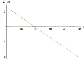
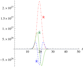
Figure 1: According to the left picture, we discover both that $H_{\lambda}\left(19.4430\,\mathrm{\zeta}\right)=0$ (i.e. $t_{0}=19.4430\,\mathrm{\zeta}$) and $\dot{\mathrm{R}}$ becomes negative immediately. The negative acceleration occurs during $17.7109\,\mathrm{\zeta}<t<21.1751\,\mathrm{\zeta}$. However, it eventually becomes positive in order to slow down scale factor shrinkage. Besides, it should be noted that the right picture only shows amounts and relationship for $\mathrm{R}$, $\dot{\mathrm{R}}$ and $\ddot{\mathrm{R}}$.

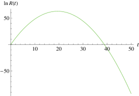
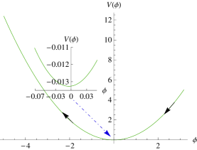
Figure 2: The scale factor shrinks to one (its initial size) again at $t=38.886\,\mathrm{\zeta}$. The time interval of both pictures is $\left[0\,\mathrm{\zeta},50\,\mathrm{\zeta}\right]$. Actually, as the sub-picture shows, the potential would be negative at $\phi\thickapprox 0$. It is almost the same period when negative acceleration occurs.

IV.2 $\boldsymbol{\phi\left(t\right)=\phi\left(t_{i}\right)\exp\left(-\frac{t-t_{i}}{\beta}\right)\cos\left[\frac{m}{\sqrt{12\pi}}\left(t-t_{i}\right)\right]}$

In this example, we set the IHP as $H\left(t_{i}\right)=14.523\,\mathrm{\zeta^{-1}}$ and discover an universe in which re-accelerated expansion will take place after the end of inflation. The results are as follows:

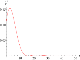
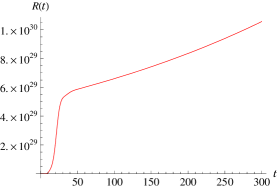
Figure 3:

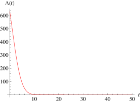
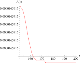
Figure 4: The cosmological term would become a non-zero positive constant of less than $1.6592\times 10^{-5}\,\mathrm{\zeta^{-2}}$ after $t\approx 173.4153\,\mathrm{\zeta}$.

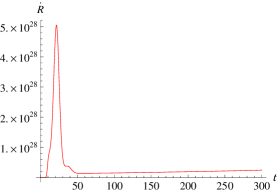
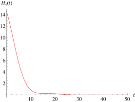
Figure 5: The end of inflation is approximately $t\thickapprox 21.5302\,\mathrm{\zeta}$ when the maximum of $\dot{\mathrm{R}}$ happens.

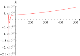
Figure 6: $\ddot{\mathrm{R}}$ is no longer less than zero after $t\thickapprox 64.3050\,\mathrm{\zeta}$.

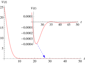
Figure 7: The time interval of both pictures is $\left[0\,\mathrm{\zeta},50\,\mathrm{\zeta}\right]$. The sub-pictures show the conditions of the minimum negative potential.

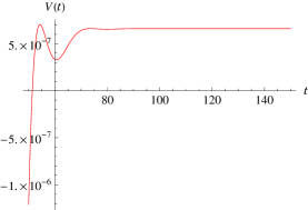
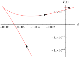
Figure 8: The time interval of both pictures is $\left[50\,\mathrm{\zeta},150\,\mathrm{\zeta}\right]$. From them, we discover that the potential will rise to positive from negative, and hold a positive value after a sufficient time has passed.

For emphasis, the important data from this example should be mentioned again: the period of the inflation is before $21.530\,\mathrm{\zeta}$; the universe has three instances of negative acceleration during $21.530\,\mathrm{\zeta}<t<64.305\,\mathrm{\zeta}$ in order to stop inflation before it immediately emerges into accelerated expansion again. In this situation, the potential would be $6.60154\times 10^{-7}\,\mathrm{\zeta^{-2}}$ when $t\gg 225\,\mathrm{\zeta}$.

IV.3 $\boldsymbol{\phi\left(t\right)=\phi\left(t_{i}\right)\exp\left(-\frac{t-t_{i}}{\beta}\right)\cos\left[\frac{m}{\sqrt{12\pi}}\left(t-t_{i}\right)\right]}$

Using the same model as in example B but with the smaller initial parameter of $H\left(t_{i}\right)=14.518\,\mathrm{\zeta^{-1}}$, we find that the scale factor shrinks after the end of inflation.

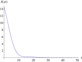
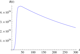
Figure 9: The end of inflation is before $t\thickapprox 21.3869\,\mathrm{\zeta}$

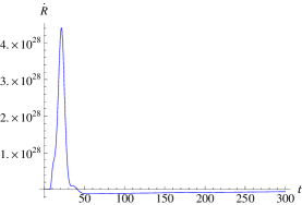
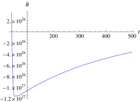
Figure 10: We discover $\dot{\mathrm{R}}\left(41.3895\,\mathrm{\zeta}\right)\thickapprox 0$ at $t_{0}\lesssim 41.3896\,\mathrm{\zeta}$ .

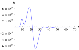
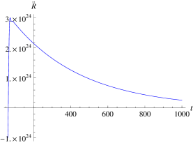
Figure 11: $\ddot{\mathrm{R}}$ is no longer less than zero after $t\thickapprox 52.4105\,\mathrm{\zeta}$.

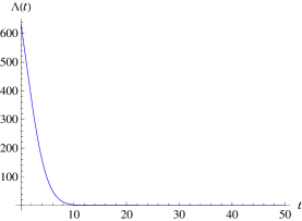
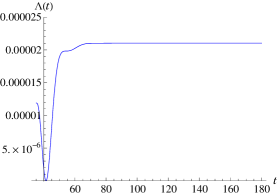
Figure 12: The cosmological term would become an approximately non-zero positive constant as $2.10405\times 10^{-5}\,\mathrm{\zeta^{-2}}$ when $t\gtrsim 173.4152\,\mathrm{\zeta}$.

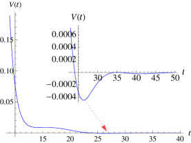
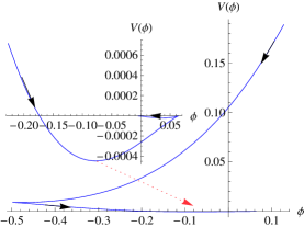
Figure 13: The time interval of both pictures is $\left[9\,\mathrm{\zeta},40\,\mathrm{\zeta}\right]$. The conditions of the minimum negative potential have been shown by sub-pictures.

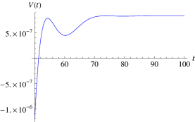
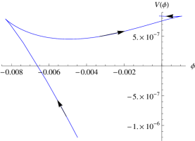
Figure 14: The time interval of both pictures is $\left[50\,\mathrm{\zeta},100\,\mathrm{\zeta}\right]$. They allow us to see that the potential will rise to positive from negative, before landing on a positive value after an adequately long period of time.

Certain important data from this example is noteworthy: the period of inflation is before $21.387\,\mathrm{\zeta}$; at $t>41.389\,\mathrm{\zeta}$, the scale factor begins to shrink, i.e. $\dot{\mathrm{R}}\left(t>41.389\,\mathrm{\zeta}\right)<0$; there are three occurrences of negative acceleration during $21.386\,\mathrm{\zeta}<t\lesssim 63.290\,\mathrm{\zeta}$ before the universe begins to experience positive acceleration, which gradually slows down the collapse. The value of its potential would be $8.37174\times 10^{-7}\,\mathrm{\zeta^{-2}}$ when $t\gg 210\,\mathrm{\zeta}$.

V discussion and summary

Analysis of units

In the previous section, we introduced the units of time “$\mathrm{\zeta}$” and mass “$\mathrm{M}$”, and fixed them as $\mathrm{M=\zeta^{-1}}$. The adoption of these settings contains two benefits: First, we can choose a proper scale for $\mathrm{\zeta}$ to fit our inference about the period of inflation. For example, due to the needs of the discussion witnessed in (12) and (27), we require the scale factor before the age of the universe reaches $t_{\mathrm{GUT}}\sim 10^{-36}\,\mathrm{s}$ to grow by a factor more than $e^{60}-e^{70}$. Therefore, we can define $\mathrm{\zeta}=10^{5}\,\mathrm{\mathit{t}_{\mathrm{Planck}}}$ $\left(\mathit{t}_{\mathrm{Planck}}\sim 10^{-44}\,\mathrm{s}\right)$ when considering the epoch of inflation at $t_{\mathrm{inf}}\sim 10^{-37}\,\mathrm{s}$. Of course, the other scale of $\mathrm{\zeta}$ can be used when inflation during other eras is explored. As such, corresponding to one’s inference, one could, for example, define $\mathrm{\zeta}=10^{-3}\,\mathrm{\mathit{t}_{\mathrm{EW}}}$ $\left(\mathit{t}_{\mathrm{EW}}\sim 10^{-11}\,\mathrm{s}\right)$ to investigate both the epoch of inflation before electroweak phase transition and the situations that arise from it. Second, a new unit of energy density can be defined corresponding to

$$\mathrm{\varepsilon_{\mathrm{\zeta}}}=\frac{3c^{2}\zeta^{-2}}{8\pi G}$$ (42)

for (35), (39), (40) and (41). Thus, if we adopt $\mathrm{\zeta}=10^{5}\,\mathrm{\mathit{t}_{\mathrm{Planck}}}$ and introduce the Planck energy density $\mathrm{\varepsilon_{\mathrm{Planck}}}=c^{2}G^{-1}\,\mathrm{\mathit{t}_{Planck}^{-2}}$ $\left(\mathrm{\varepsilon_{\mathrm{Planck}}}\sim 10^{117}\,\nicefrac{\mathrm{GeV}}{\mathrm{cm^{3}}}\right)$, we attain $\varepsilon_{\mathrm{\zeta}}=\frac{3}{8\pi}\times 10^{-10}\,\mathrm{\varepsilon_{\mathrm{Planck}}}$. Applications of unit-setting for previous tests will be presented in the appendix.

Data analysis

According to (32), (33) and (34), the evolution of $\int_{t_{i}}^{t}\dot{\phi}^{2}d\tau$ is an important key for controlling any of the types of universe outlined in Table I. Therefore, as an universe of type 1 or 2, if it has a non-resting kinetic scalar field at $t>t_{0}$ that leads (36) or the square root of (33) to be negative, this value will always be negative and the universe will collapse forever, even though the density of its ordinary matter is extremely thin at the time. However, if the $\dot{\phi}$ goes to rest quickly enough, causing (34) and (36) to both become positive constants, the universe(s) that we place it in type 4 will be in a state of accelerating expansion. Additionally, if $\int_{t_{i}}^{t}\dot{\phi}^{2}d\tau$ is sufficiently small for a long enough time to lead (36) to be positive, the universe(s) will be expanding but with uncertain behavior as in type 5. The reason for this uncertainty is the fact that we can not have an exact value for $4\pi\dot{\phi}^{2}$ in (34). To compare, the static type 3 universe(s) as displayed in Table I would occur with extreme difficulty because a fine-tuned $\dot{\phi}^{2}\left(t\right)$ is needed to make $H\left(t_{i}\right)-4\pi\int_{t_{i}}^{t>t_{r}=t_{0}}\dot{\phi}^{2}d\tau=0$. This is most unnatural.

Moreover, we discover that $\ddot{\mathrm{R}}$ of (34) will always be positive after a characteristic time $t_{*}$, even if/when the universe finally shrinks! This has been verified by our tests and is expressed in Table I as a collapsed universe of type 1 or 2 (as in figure 11), and an expanded universe of type 4 (as in figure 6). It looks highly counterintuitive, but a collapsed universe could only have an epoch of “decelerated collapse” if $t_{*}$ was near to $t_{0}$ and $t_{0}$ big enough to allow it a very low matter-density. By way of contrast, it seems that the type 5 universe should not rightly be in Table I because, unlike the other types of universe, its time period for observation is before the characteristic time $t_{0}$ or $t_{r}$. However, type 5 is absolutely necessary: without it, our information regarding universes of other types would be incomplete because we would be unable to investigate them with either decelerating expansion or both accelerating and decelerating expansion in rotation.

For explanatory convenience, slightly exaggerated values for the IHPs are introduced in examples B and C so as to show the accelerating expansion and collapse of the universe clearly. Following this technique, we discover that if we wish to have an e-folding number $N\sim 60-70$ for the model $\phi\left(t\right)=\phi\left(t_{i}\right)\exp\left(-\frac{t-t_{i}}{\beta}\right)\cos\left[\frac{m}{\sqrt{12\pi}}\left(t-t_{i}\right)\right]$, $H\left(t_{i}\right)$ must have a value close to $14.52\,\mathrm{\zeta^{-1}}$ with initial settings in line with those mentioned at the beginning of Section IV. Actually, such a value seems to be particularly special because the universe collapses when it is placed at $H\left(t_{i}\right)=14.518\,\mathrm{\zeta^{-1}}$ and enters a situation of accelerating expansion if it is set as $H\left(t_{i}\right)=14.523\,\mathrm{\zeta^{-1}}$. Although these two examples are toy models, a critical value for the IHP can be determined at about $H\left(t_{i}\right)\gtrsim 14.52064830064115\,\mathrm{\zeta^{-1}}$ for the model as currently proposed. This is according to the conditions of $N\gtrsim 60-70$ and the real cosmological constant $\Lambda\thickapprox 1.934\times 10^{-35}\,\mathrm{s^{-2}}$. Besides, we discover that the circumstances of inflaton mass $m$ and the decay parameter $\beta$ are also essentials for controlling an universe, regardless of whether it is expanded or collapsed. Indeed, as outlined above, when $m$ and $\beta$ are fixed, a big enough value for $H\left(t_{i}\right)$ would make an universe enter accelerating expansion after inflation. However, a bigger $m$ or $\beta$ with a fixed $H\left(t_{i}\right)$ would finally lead an universe to collapse.

To enlarge, according to (34) and (35), the behavior of $V\left(t\right)$ is analogous to $\nicefrac{{\ddot{\mathrm{R}}}}{{\mathrm{R}}}$, so the potential value will always be positive after a suitably long time for any universe of types 1, 2 or 4. Of course, the minimum of $V\left(t\right)$ does not occur at $t>t_{r}$, but at the time when an universe has a maximum deceleration of $\mathrm{R}\left(t\right)$ in order to stop inflation. This conforms to figure 15 at $t\approx 32\,\mathrm{\zeta}$. On the other hand, we find that the potential could be a surjective function of $\phi$ which is according to figures 7 and 8 of example B and figures 13 and 14 of example C. Actually, the reason for this is that the potential $V$ should be a function with variables of $\phi$ and $t$, as seen in (16) and (31). From these figures, we can understand that $V$ would hit a minimum negative value and then rise to a positive one proportional to $\Lambda$ when $\dot{\phi}$ is finally at rest. This is quite different from the phase transition model that we are familiar with and it looks as if it would correspond to the scenario of reheating after inflation.

Additionally, we have found that, from determining the value of the cosmological constant alone, it is impossible to make conclusions about the denouement of any universe except a static one. Fortunately, the $\Lambda-t$ picture does contain an indication that could help us to differentiate between collapsing and expanding universes though: as figure 16 displays, there is a rule whereby an universe would be collapsing if $\Lambda$ increases from lowest point, i.e. zero (as depicted by the red, solid line), but expanding when $\Lambda$ decreases smoothly (as depicted by the blue, dotted line).

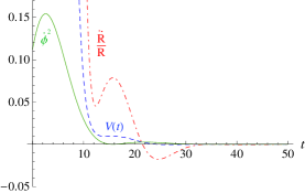
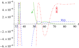
Figure 15: The above pictures show the behavior of $\nicefrac{{\ddot{\mathrm{R}}}}{{\mathrm{R}}}$, $\dot{\phi}^{2}$ and $V\left(t\right)$ in test B.

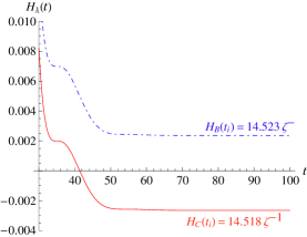
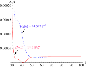
Figure 16: These show the behavior of $H_{\lambda}\left(\zeta\right)$ and $\Lambda\left(\zeta\right)$ of type 2 (with a blue, dot-dashed line) and type 4 (with a solid, red line) universes.

Answers to the Aforementioned Problems

In this article, we have obtained the differential equation (31) according to our assumption of the necessary time-varying scalar field potential and found that the term of $-3H\dot{\phi}^{2}$ could absorb energy from the total energy density difference of inflaton. Of course, we could use the conventional method to calculate (28), (29) and (30) or (31). This is done by proposing an ansatz for the potential so as to obtain the solutions of inflaton and the scale factor of an universe. Through an analysis of the solutions gained from this process, we are able to answer corresponding questions about the growth of an universe.

Irrespective of the above practice, however, we have decided to employ a new and non-traditional method for solving equations and problems – one which gives the ansatz of $\phi\left(t\right)$ that appears in the solution of the scale factor as (32) directly. Using the scale factor gained in this manner, we can then “rebuild” the potential function as (35) according to the ansatz of $\phi\left(t\right)$. In other words, with the non-traditional method, potential is replaced by the scalar field for the role of the ansatz.

The new method does not refute the traditional one, but rather contains its own advantages: by testing A, B and C, we achieve a feasible method for analyzing simple solutions of inflaton that are otherwise dependent on highly complex potential models. Moreover, besides toy-model tests, the evolution of the inflaton potential energy density (IPED) can also be easily realized through the careful observation and analysis of (35). From this, it is clear to see that, apart from being constrained by $\int_{t_{i}}^{t}\dot{\phi}^{2}d\tau$, the IPED is also restricted by the initial Hubble parameter $H\left(t_{i}\right)$. The fact that our proposal enables us to obtain the IHP is a very important advantage because its corresponding term, as shown in (40), can be viewed as the vacuum energy density of the universe’s original situation. Furthermore, we can assert that (41) is Einstein’s cosmological term, making (39) the effective cosmological constant as needed.

Thus, we have proposed a scheme that enables a solution to the problem of the cosmological constant: as long as suitable models of inflaton are given with a value for the e-folding number as desired, and regardless of whether these models are based on intuition or observation, we will be able to obtain the corresponding IHP by inputting the present observation of the Hubble constant. This then allows solutions for the evolution of IPED to be uncovered. Finally, we can solve the problems of the cosmological constant by considering the evolution of the total energy density of inflaton according to (29), (33), (39), (40) and (41).

At this stage, let us quickly review the Friedmann equations in terms of matter density and pressure with the cosmological constant:

$$\frac{\ddot{\mathrm{R}}}{\mathrm{R}}=-\frac{4\pi G}{3c^{2}}\left(\varepsilon_{\mathrm{matter}}+3p\right)+\frac{\Lambda c^{2}}{3},$$ (43)

$$\left(\frac{\mathrm{\dot{R}}}{\mathrm{R}}\right)^{2}=\frac{8\pi G}{3c^{2}}\varepsilon_{\mathrm{matter}}+\frac{\Lambda c^{2}}{3}.$$ (44)

Now, (43) is adequate for explaining/describing the re-accelerating expansion of an universe with its consideration of the cosmological constant’s existence or/and the negative pressure of the universe. However, problems ensue when (44) is analyzed: while it yields suitable results for the present moment in the present universe, it struggles to adequately illustrate a situation in which a collapse occurs from an expanding universe. In my opinion, this predicament constitutes a very big loss to the whole theory of cosmology, especially since we can only explore other kinds of universe in our imagination and require equations that can help us to do so. This is why our new, non-conventional method is particularly useful as it facilitates such theoretical exploration.

Alongside our findings, two additional facts about the evolution of an universe can be established. First, when an universe appears to be expanding at time $t$, $H\left(t_{i}\right)$ must be bigger than the effect of $\int_{t_{i}}^{t}\dot{\phi}^{2}d\tau$; conversely, when a collapsing universe is considered at $T$, $\int_{t_{i}}^{T}\dot{\phi}^{2}d\tau$ will be bigger than $H\left(t_{i}\right)$, if $\dot{\phi}$ is still moving at this time. This is a natural conclusion emerging from (36) because $\int_{t_{i}}^{t}\dot{\phi}^{2}d\tau$ grows with time. It consequently follows that if one can give correct information about $\dot{\phi}^{2}$ at an arbitrary cosmic time $t$, (36) can be used to describe the evolution of an universe coherently and not only in an expanding situation, but also in a collapsing one. For this reason, our proposal is a better alternative than the traditional method because it gets rid of the predicament that emerges from the Friedmann equation (44).

The second fact is as follows: according to (35), we discover that it could be possible to have a negative value of potential, such as in the situation of $\dot{\phi}^{2}\left(t_{0}\right)>0$. We should point out that the negative value appears to disprove our proposal. Fortunately, however, the catastrophe is averted because a negative value for the total energy density of inflaton will not be possible when its dependence on the property of (35) is incorporated. Indeed, the negative potential actually has an advantage because it combines with $\dot{\phi}^{2}$ in (28) to allow a large enough deceleration for the purpose of ending the period of inflation. Traditionally, $\dot{\phi}^{2}$ has been problematic because it requires an extremely specific/fine-tuned value that makes the universe become the one what we see today. Accordingly, a negative potential could help $\dot{\phi}^{2}$ to have more possibility during the end of the inflation. Moreover, the range of running potential from positive to negative could also help acceleration to smoothly move between positive and negative as well. This provides an adequate picture of the universe’s evolution.

As such, the two facts that we have proposed are thus mechanisms that can fulfill the necessities of both collapsing and re-accelerating expanding-type universes. Importantly, we can assert that, with a proper model $\phi$ and our proposal from (33) to (41), the introduction of these two facts will cause the gulf between theories to disappear.

In reference to our discussion, the appendix provides much important information about our tests while adopting units with which we are familiar. It deserves to be mentioned that rows $\dagger$ and $\ddagger$ show the corresponding properties of the current cosmological constant, which are made by calculating with the approximation of $H\left(t_{i}\right)=14.52064830064116\,\mathrm{\zeta^{-1}}$ and the same model $\phi$ as with test B.

appendix

	$t_{e}$	$t_{0}$	$t_{*}$
Test A	$9.548\times 10^{-38}$	$1.048\times 10^{-37}$	$1.142\times 10^{-37}$
Test B	$1.161\times 10^{-37}$	none	$3.467\times 10^{-37}$
Test C	$1.153\times 10^{-37}$	$2.231\times 10^{-37}$	$2.826\times 10^{-37}$
$\dagger$	$1.157\times 10^{-37}$	none	$1.632\times 10^{-37}$

Table 2: The unit of time in this table is “$\mathrm{s}$”. Where $t_{e}$ is the time when inflation in the universe has ended; $t_{0}$ is the time when $\dot{\mathrm{R}}$ becomes negative; and $t_{*}$ is the time when $\ddot{\mathrm{R}}$ is no longer negative. The unit of time that we adopted is $\mathrm{\zeta}=10^{5}\,\mathrm{\mathit{t}_{\mathrm{Planck}}}$.

	$\left\langle\varepsilon_{\mathrm{vac}}\right\rangle$	$\left\langle\varepsilon_{\mathrm{V}}\right\rangle_{initial}$	$\left\langle\varepsilon_{\mathrm{V}}\right\rangle_{min}$	$\left\langle\varepsilon_{\mathrm{V}}\right\rangle_{final}=\left\langle\varepsilon_{\Lambda}\right\rangle$
Test A	$1.450\times 10^{108}$	$1.446\times 10^{108}$	$-3.836\times 10^{105}$	none
Test B	$7.281\times 10^{108}$	$7.265\times 10^{108}$	$-1.133\times 10^{104}$	$1.909\times 10^{101}$
Test C	$7.276\times 10^{108}$	$7.260\times 10^{108}$	$-1.289\times 10^{104}$	$2.421\times 10^{101}$
$\ddagger$	$\lesssim 7.279\times 10^{108}$	$\lesssim 7.263\times 10^{108}$	$\lesssim-1.207\times 10^{104}$	$2.732\times 10^{78}$; $6.468\times 10^{-6}$ $\star$

Table 3: The unit of energy density is “$\nicefrac{\mathrm{GeV}}{\mathrm{cm^{3}}}$”. We can calculate the initial energy density by (40) and the minimum potential energy density and energy density of $\Lambda$ by (35) and (39) respectively. Additionally, with regard to $\left\langle\varepsilon_{\mathrm{V}}\right\rangle_{initial}=\left\langle\varepsilon_{\mathrm{vac}}\right\rangle-\frac{1}{2}\dot{\phi}^{2}\left(t_{i}\right)$; $\star$, the upper value is calculated by using $H\left(t_{i}\right)=14.52064830064116\,\mathrm{\zeta^{-1}}$; the lower value is obtained through the current cosmological constant $\Lambda\thickapprox 1.934\times 10^{-35}\,\mathrm{s^{-2}}$.

- (1) S. Perlmutter et al., Astrophys. J. 517: 565 (1999)
- (2) A. G. Riess et al., Astron. J. 116: 1009 (1998)
- (3) P. Astier et al., A&A 447: 31 (2006)
- (4) A. G. Riess et al., Astrophys. J. 659: 98 (2007)
- (5) D. N. Spergel et al., Astrophys. J. Suppl. 170: 377 (2007)
- (6) M. Tegmark et al., Phys. Rev. D 74: 123507 (2006)
- (7) J. Frieman, M. Turner and D. Huterer, Ann. Rev. Astron. Astrophys. 46: 385 (2008)
- (8) L. M. Krauss and M. S. Turner, Gen. Rel. Grav. 27: 1137 (1995)
- (9) J. P. Ostriker and P. J. Steinhardt, Nature 377: 600 (1995)
- (10) A. R. Liddle, D. H. Lyth, P. T. Viana and M. White, Mon. Not. Roy. Astron. Soc. 282: 281 (1996)
- (11) R. R. Caldwell, R. Dave and P. J. Steinhardt, Phys. Rev. Lett. 80: 1582 (1998)
- (12) J-A. Gu and W-Y. P. Hwang, Phys. Lett. B 517: 1 (2001)
- (13) L. A. Boyle, R. R. Caldwell and M. Kamionkowski, Phys. Lett. B 545: 17 (2002)
- (14) R. R. Caldwell, Phys. Lett. B 545: 23 (2002)
- (15) A. Einstein, Sitzungsbe. K. Akad. 6: 142 (1917)
- (16) S. M. Carroll and W. H. Press, Annu. Rev. Astron. Astrophys. 30: 499 (1992); S. M. Carroll, Living Rev. Relativity 3: 1 (2001)
- (17) N. Straumann, arXiv:gr-qc/0208027v1 (2002)
- (18) J-R. Choi, C-I. Um and S-P. Kim, J. Korean Phys. Soc. 45: 1679 (2004)
- (19) G. E. Marsh, arXiv:0711.0220v2 [gr-qc] (2007)
- (20) P. Chen, arXiv:1002.4275v2 [gr-qc] (2010)
- (21) W. de Sitter, Mon. Not. R. Astron. Soc. 78: 3 (1917)
- (22) S. Weinberg, Rev. Mod. Phys. 61: 1 (1989)
- (23) E. Hubble, Proc. N. A. S. USA 15, 3: 168 (1929)
- (24) G. Lemaître, Annales de la SociétScientifique de Bruxelles 47: 49 (1927)
- (25) G. Gamow, Phys. Rev. 74 (4): 505 (1948)
- (26) G. Gamow, Nature 162: 680 (1948)
- (27) R. A. Alpher and R. C. Herman, Phys. Rev. 74 (12): 1737 (1948)
- (28) A. D. Linde, Lect. Notes Phys. 738: 1 (2008)
- (29) G. t Hooft, Nucl. Phys. B79: 276 (1974)
- (30) Ya. Zel’dovich and M. Yu. Khlopov, Phys. Lett. B79: 239 (1978)
- (31) A. D. Linde, JETP Lett. 19: 183 (1974)
- (32) A. A. Starobinsky, JETP Lett. 30: 682 (1979); A. A. Starobinsky, Phys. Lett. B 91: 99 (1980)
- (33) A. H. Guth and S. Tye, Phys. Rev. Lett. 44: 631 (1980)
- (34) A. H. Guth, Phys. Rev. D 23: 347 (1981)
- (35) S. W. Hawking, I. G. Moss and J. M. Stewart, Phys. Rev. D 26: 2681 (1982)
- (36) A. H. Guth and E. J. Weinberg, Nucl. Phys. B 212: 321 (1983)
- (37) A. D. Linde, Phys. Lett. B 108: 389 (1982); A. D. Linde, Phys. Lett. B 114: 431 (1982); A. D. Linde, Phys. Lett. B 116: 340 (1982); A. D. Linde, Phys. Lett. B 116: 335 (1982)
- (38) A. Albrecht and P. J. Steinhardt, Phys. Rev. Lett. 48: 1220 (1982)
- (39) V. F. Mukhanov and G. V. Chibisov, JETP Lett. 33: 532 (1981)
- (40) S. W. Hawking, Phys. Lett. B 115: 295 (1982)
- (41) A. A. Starobinsky, Phys. Lett. B 117: 175 (1982)
- (42) A. H. Guth and S. Y. Pi, Phys. Rev. Lett. 49: 1110 (1982)
- (43) J. M. Bardeen, P. J. Steinhardt and M. S. Turner, Phys. Rev. D 28: 679 (1983)
- (44) V. F. Mukhanov, JETP Lett. 41: 493 (1985); V. F. Mukhanov, Physical Foundations of Cosmology (Cambridge University Press, Cambridge, 2005)
- (45) A. R. Liddle and D. H. Lyth, Cosmological Inflation and Large-Scale Structure (Cambridge University Press, Cambridge, 2000)