The nature of the different zero-temperature phases in discrete two-dimensional spin glasses: Entropy, universality, chaos and cascades in the renormalization group flow

Abstract

The properties of discrete two-dimensional spin glasses depend strongly on the way the zero-temperature limit is taken. We discuss this phenomenon in the context of the Migdal-Kadanoff renormalization group. We see, in particular, how these properties are connected with the presence of a cascade of fixed points in the renormalization group flow. Of particular interest are two unstable fixed points that correspond to two different spin-glass phases at zero temperature. We discuss how these phenomena are related with the presence of entropy fluctuations and temperature chaos, and universality in this model.

Since the beginning of the study of disordered systems with renormalization and scaling methods the question of universality and of the relevance of the realization of the disorder have been a key issue [1]. Why indeed should we accept that some abstract models are the archetype of a very broad class of systems if their behavior depends drastically on tiny details? The Edwards-Anderson [2] model is one of the models that are widely regarded as a prototype of disordered systems in statistical physics. It is an Ising model with disordered and competitive interactions and has been the source of many surprises and developments in the last thirty years [3, 4].

Its two-dimensional (2D) version, one of its simplest settings, has very special properties with respect to universality. It is now agreed that the spin-glass phase exists only at zero temperature [5, 6, 7], where the spin-glass susceptibility diverges. However, the behavior of the model seems to depend drastically on microscopic details and in particular discrete and continuous couplings leads to different properties [8, 9] at zero temperature. On the other hand, for nonzero temperatures, strong evidence for universal critical behavior has been observed [10, 11, 12]. This rises questions on the very nature of universality, if any, in strongly disordered bidimensional systems. Why such a difference? What are the mechanisms behind this behavior? The key to understand these features lies in the difference between strictly zero and vanishing temperature [13, 14]. When temperature is finite, entropy fluctuations play a major role and, for large enough sizes, bring back discrete models to the continuous class [10]. These mechanisms were further exploited in [15], with a special emphasis on the so-called temperature chaos effect [16, 17, 18].

In this Letter we study the behavior of continuous and discrete 2D spin glasses in the context of the Migdal-Kadanoff renormalization group (MKRG) [19]. We observe that indeed continuous and discrete $2D$ spin glasses are eventually associated with the very same physically relevant fixed point. However, there are also key differences that are the consequence of a cascade of two repulsive fixed points in the MKRG flow in the case of the discrete model. In a real-space picture, these phenomena are associated with two different temperature-dependent crossover length scales, so that two different zero-temperature spin-glass phases can be observed depending on the system size $L$ and the temperature $T$.

This Letter is organized as follows: first, we define the model and recall briefly the MKRG. We then study the MKRG flow and observe one attractive paramagnetic fixed point and two repulsive ones corresponding to the $T=0$ discrete and continuous classes, respectively. We discuss the crossover length scales between different regimes, the cascade of fixed points and its effects on effective critical exponents which may easily camouflage the fact that the critical behavior of the 2D spin glass is universal.

1 Two-dimensional spin glasses

The Hamiltonian of the Edwards-Anderson Ising spin glass[2] is given by

$${\mathcal{H}}=-\sum_{<i,j>}J_{ij}S_{i}S_{j}.$$ (1)

The spins $S_{i}$ lie on a square lattice of size $N=L^{2}$ in two space dimensions and the interactions between the spins are between nearest neighbors. We shall consider two different models: in the discrete one, the interactions are chosen randomly as $J_{ij}\in\{\pm 1\}$ while in the continuous, or Gaussian model, we shall use a Gaussian distribution of the $J_{ij}$ with zero mean and unit variance, instead.

It is by now generally accepted (although there is no rigorous proof of this, but see[20]) that there is no spin-glass transition at finite temperature in both cases. Instead, the spin-glass susceptibility diverges when $T\to 0$ and the spin-glass phase exists only at zero temperature. At any finite temperature, however, this implies the existence of an equilibrium length scale $\xi_{\rm eq}(T)$ beyond which the spin-glass correlation decays exponentially fast and the system is effectively in a paramagnetic state. For length scales below $\xi_{\rm eq}(T)$, the correlation function decays only as a power-law and the system has a spin-glass-like correlation. If one is looking at a system of size $L\ll\xi_{\rm eq}(T)$, it thus looks very much as a spin glass (it has power-law correlations) and only for larger sizes, when $L\gg\xi_{\rm eq}(T)$ does the system finally look paramagnetic.

2 Migdal-Kadanoff renormalization group

Low-dimensional systems are often well described by the Migdal-Kadanoff renormalization group and 2D spin glasses are no exception [19, 21, 22, 23]. We shall thus work within the MKRG approach and study how different are 2D discrete and continuous spin glasses. For a disordered system such as a spin glass, the MKRG is a functional renormalization group method, as the quantity that is being renormalized is the distribution of couplings $P(\beta J)$. Starting from a given inverse temperature $\beta=1/T$ and an initial distribution of couplings $P_{\rm init}(\beta J)$, MKRG allows to follow the (approximate) flow under renormalization (for a detailed description see for instance [21, 22, 23]). There are many ways to write the MKRG recursion for 2D spin glasses. We shall follow [9] and use the recursion on a hierarchical lattice with $b=3$ branches and $s=3$ spins per branch yielding a model with effective dimension $D=2$:

$$P^{G+1}(\beta J)\!\!=\!\!\int\!\!\prod_{i=1}^{9}\left(d\beta_{i}P^{G}(\beta J_{i})\right)\delta{[\beta J\!-\!{\cal{F}}(\{{\beta J_{i}\}}_{i=1\ldots 9})]}$$ (2)

$$\mbox{with~{}~{}~{}}{\cal{F}}(\{{\beta J_{i}\}}_{i=1\ldots 9}) = \mbox{atanh}({\tanh{\beta J_{1}}\tanh{\beta J_{2}}\tanh{\beta J_{3}}})\phantom{.}$$

$$+ \mbox{atanh}({\tanh{\beta J_{4}}\tanh{\beta J_{5}}\tanh{\beta J_{6}}})\phantom{.}$$

$$+ \mbox{atanh}({\tanh{\beta J_{7}}\tanh{\beta J_{8}}\tanh{\beta J_{9}}}).$$

This recursion can be implemented trivially using population dynamics. It is also sometimes convenient to see the MKRG as an exact solution on a hierarchical lattice [24]. In this case one interprets the “time” in the RG flow (that is, the index $G$ in Eq. 2) as related to the effective size of the system via $L=3^{G}$. This allows to characterize length scales in the system, and it also provides an exact realization of the droplet/scaling theory [16, 17, 18], which is, at least for the $2D$ model, accepted to be a good description.

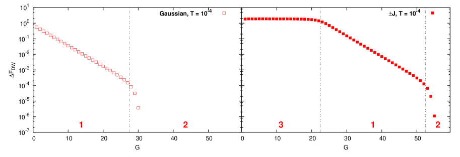
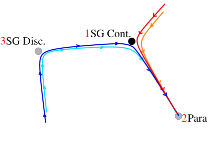
Figure 1: Top: The domain-wall free energy $\Delta F_{\rm DW}=\sqrt{\langle(J_{\rm p}-J_{\rm a})^{2}\rangle}$ associated with an effective bond after $G$ MKRG iterations (where the effective size of the system is $L=3^{G}$), in the low-temperature phase of the Gaussian (left) and binary (right) spin glasses. In the Gaussian case one is in the spin-glass phase where $\Delta F_{\rm DW}\propto 3^{\theta G}$, with $\theta\approx-0.278$ until the effective size of the system is larger than a crossover length $\xi_{\rm eq}(T)=T^{-\nu}$ where the system becomes paramagnetic and $\theta=-\infty$. In the discrete case, the system is first in a phase where $\theta^{\prime}=0$, until a first length scale $\ell_{{\rm c}}$ is crossed, and only at this point it decays with the continuous exponent $\theta\approx-0.278$. When the effective system is even larger, such that $L\gg L_{\rm G}\propto T^{-\nu_{\rm eff}}$, the system becomes again paramagnetic: there are therefore two different spin-glass phases in the zero-temperature limit. Bottom: the corresponding flow in the MKRG with the three different fixed points. Binary spin glasses are cascading through the three fixed points.

3 Gaussian couplings

When starting from a Gaussian distribution $P_{\rm{init}}(\beta J)$ at low temperature, the MKRG flows to a symmetric slightly non-Gaussian distribution with zero mean and a variance decaying with $G$ such that $\langle J^{2}\rangle\propto L^{\theta}$, where ${\theta}\approx-0.278$. At strictly $T=0$, this is the strong-coupling fixed point describing the continuous spin-glass phase, but at any finite temperature $T$ the fact that $\theta<0$ implies that the bonds are not robust and that the spin-glass phase does not survive (and that the fixed point is unstable). This is precisely what happens once enough recursions are performed and the MKRG flows to a trivial delta function exponentially fast: this is the stable paramagnetic pseudo-fixed point where formally ${\theta}=-\infty$ (see Fig. 1 and Fig. 2.)

Following the standard droplet interpretation, scaling relations can be obtained by realizing that the thermodynamic behavior is dominated by large excitations (the droplets) of size $\ell$ and $O(1)$-energy that can be found with a probability scaling as $\ell^{\theta}$. The probability that two spins at distance $r$ are correlated thus decays as $r^{\theta}$ and this will be on the order of the thermal fluctuations when $r$ reaches the equilibrium length scale $\xi_{\rm eq}\propto T^{1/\theta}$. In other words the correlation function behaves as $C_{\rm Gauss}(r,T)\propto r^{\theta}e^{-r/\xi_{\rm eq}(T)}$ which indicates that the critical exponent for the correlation length is simply $\nu=-1/\theta$. Indeed, when performing the MKRG at finite $T$, we observe that when the effective size $L$ is of the order of $\xi$ (which eventually happens for any positive temperature, provided we do enough recursions), the value of $\theta$ drops from $-0.278$ to $-\infty$. This is the sign that we are now in the paramagnetic phase and that there are no correlations beyond the scale $\xi_{\rm eq}(T)$ (see again Fig. 1).

We recall all the MKRG exponents for the Gaussian model, together with the estimated ones from the $2D$ square lattice in Table 1. The values are very close, showing that the critical properties are well captured by the MKRG approximation.

	MK	2D
$\theta$	-0.278	-0.287 [25]
$\nu=-1/\theta$	3.597	3.48
$d_{s}$	1	1.28 [26, 27]
$\zeta=\frac{d_{S}}{2}-\theta$	0.778	0.927

Table 1: Gaussian couplings: critical exponents from the MKRG approximation and the 2D square lattice.

4 Discrete spin glasses

The discrete $\pm J$ model displays a more puzzling phenomenology. It was first realized that strictly at zero temperature, one finds $\theta^{\prime}=0$ (we shall use a prime for all exponents in the discrete model that are related with this fixed point, that we will refer to as the discrete fixed point), both in MKRG [9] and in the 2D model [8], suggesting a different universality class with respect to Gaussian disorder. However, it was soon realized that a small perturbation (such as discrete, but fractional couplings) were enough to destabilize this fixed point, and the MKRG was then flowing to the continuous one [9] where $\theta=-0.287$. Subsequent Monte-Carlo simulations of the 2D model indicated that some observables were in the same universality class in both the discrete and continuous models[10]. This rises questions: how one goes from different results at zero temperature in the discrete and the continuous model to the same ones at finite $T$? We will see that there are actually two different unstable fixed points, corresponding to two different spin-glass phases, that can be observed depending on how the $T=0$ limit is taken, and a stable pseudo-fixed point corresponding to the paramagnetic phase.

4.1 The zero-temperature discrete phase

We first repeat the $T=0$ analysis of [9] and, indeed, find $\theta^{\prime}=0$. That means that the $P^{G}(J)$ (which we rewrite in order to remove the dependence in $\beta$ by taking formally the limit $\beta\to\infty$ in Eq. 2) converges to a nontrivial function that does not evolve under renormalization. This fixed point thus describes a zero-temperature spin-glass phase, whose properties are different from the ones seen in the Gaussian model.

The nontrivial phenomenon, however, is that the flow is not going directly to the paramagnetic pseudo-fixed point, but instead it is first governed by the continuous fixed point, and then finally flows to the paramagnetic one (see Fig. 1) implying a nontrivial cascade in the MKRG flow.

	MK	2D
$\theta^{\prime}$	0	0
$\nu^{\prime}=1/\zeta^{\prime}$	2.597	1.43 …1.83
$d_{s}^{\prime}$	0.77	1.095 …1.395 [28]
$\zeta^{\prime}=\frac{d_{S}^{\prime}}{2}$	0.385	0.5 …0.7
$\nu_{\rm eff}=\nu+\nu^{\prime}$	6.195	4.9 …5.5

Table 2: Discrete $\pm J$ couplings: critical exponents associated with the “discrete” fixed point in the MKRG approximation and the estimated ones from the 2D square lattice. The exponent $\nu_{\rm eff}$ describes the divergence of the spin-glass correlation length using a scaling in the system size $L$ and the bare temperature $T$.

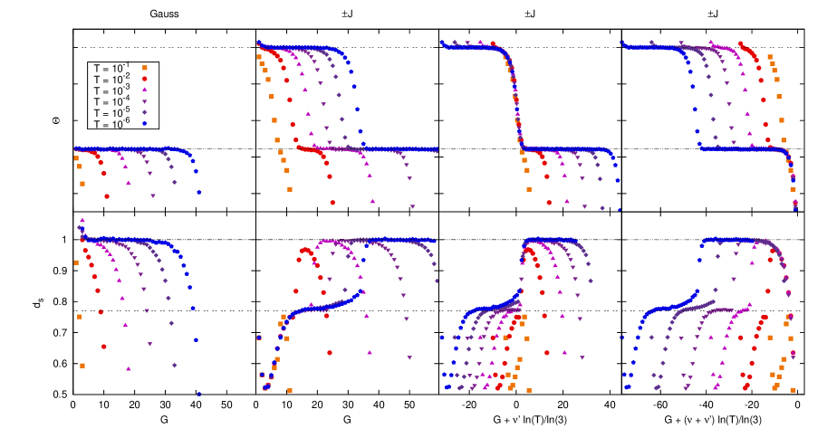
Figure 2: (Color online) Effective $\theta$ and fractal dimension of domain walls $d_{s}$ for the Gaussian and $\pm J$ models as a function of the number of generations $G$ in the MKRG for different temperatures $T$. The length scale probed by the MKRG is $L=3^{G}$. For the discrete model, the rescaling using the exponent $\nu^{\prime}=1/\zeta^{\prime}$ allows to superimpose the curves in the crossover region from the discrete to the continuous fixed point, while using $\nu_{\rm eff}=\nu+\nu^{\prime}$ one can superimpose the crossover from the continuous fixed point to the paramagnetic region.

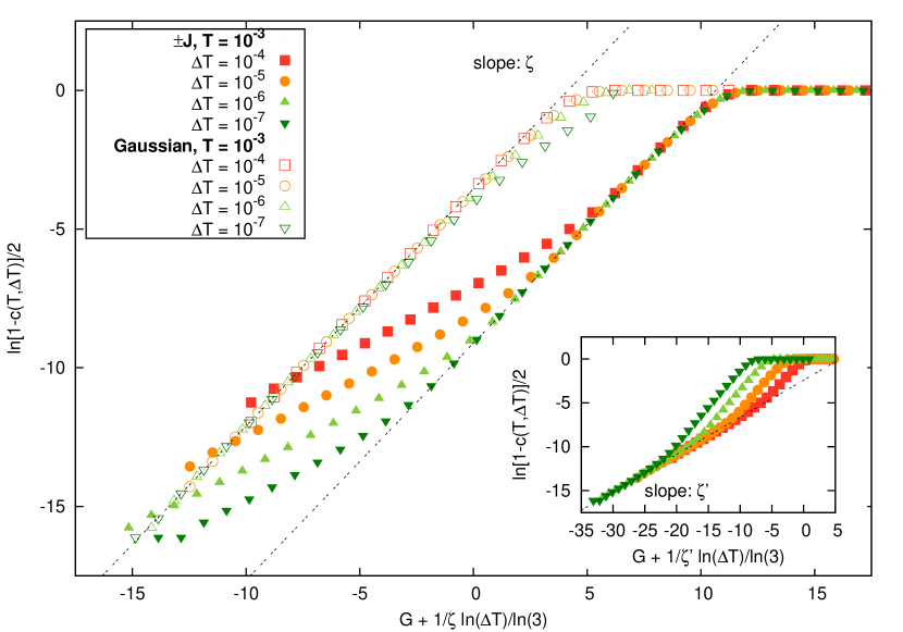
Figure 3: (Color online): Temperature chaos in 2D spin glasses: we show $\ln(1-C(T,\Delta T))/2$ where $C(T,\Delta T)$ is the correlation between the couplings at temperature $T$ and $T+\Delta T$. In the Gaussian model, the system is characterized by a critical exponent $\zeta$, while in the binary case one can observe either the exponent $\zeta$ or $\zeta^{\prime}$ depending on the values of $L$ and $T$.

4.2 Entropic fluctuations and temperature chaos

The reasons behind the instability of the discrete fixed point are, as first discussed by [10], entropic fluctuations that at any finite temperature make the zero-temperature and the vanishing-temperature limits different (a very similar phenomenon appears in diluted $3D$ spin glasses [14], where the critical dilution calculated by first setting the temperature to zero and then taking the system size to infinity is strictly larger than when first taking the system size to infinity at finite temperature and then taking the temperature to zero). This is in fact deeply connected with the notion of temperature chaos[15, 16, 17, 18, 24, 29, 30].

Equilibrium states of spin glasses are sensitive even to very small perturbations. Let us repeat here the classical thermodynamic argument of [16, 18]. Consider a spin glass in the scaling/droplet approach: take two equilibrium states at temperature $T<T_{{\rm c}}$ differing by a very large droplet of characteristic size $\ell$. Then the two states have free energies that differ by $\Delta F(T)=\Delta E-T\Delta S\approx\Upsilon(T)\ell^{\theta}$, where $\Upsilon(T)$ is the energy stiffness coefficient. When one changes the temperature by $\Delta T$, then $\Delta F(T+\Delta T)\approx\Delta E-(T+\Delta T)\Delta S$ so that $\Delta F(T+\Delta T)\approx\Upsilon(T)\ell^{\theta}-\Delta T\Delta S$. In this phenomenological approach, the entropy difference is associated with the droplet’s surface so that $\Delta S$ has a random sign and a typical magnitude $\sigma(T)\ell^{d_{{\rm s}}/2}$, where $\sigma(T)$ is called the entropy stiffness and $d_{{\rm s}}$ is the fractal dimension of the droplet’s surface. If $d_{{\rm s}}/2>\theta$, which follows from droplet theory, then $\Delta F(T+\Delta T)$ can change sign between T and $T+\Delta T$ for length scales greater than

$$\ell_{{\rm c}}\propto\bigg{(}\frac{\Upsilon(T)}{\sigma(T)\Delta T}\bigg{)}^{1/{\zeta}}$$ (3)

with $\zeta=d_{{\rm s}}/2-\theta$. This can be checked in the MKRG using the correlation between the effective couplings between the border spins at different temperatures

$$C(T,\Delta T)=\frac{\langle J(T)J(T+\Delta T)\rangle}{\langle J(T)\rangle\langle J(T+\Delta T)\rangle}.$$ (4)

Besides the scaling in $L/\ell_{{\rm c}}$, it is also expected[30] that for small values of $\Delta T$ one has $1-C\propto L^{2\zeta}$. As shown in Fig. 3 we find that indeed one can rescale the curves and observe the predicted slope using $\zeta=0.78$ for the Gaussian system. Using the definition of $\zeta$, this shows that $d_{s}=1$ in MKRG, as is widely accepted. For the discrete case, however, we first find a $\zeta^{\prime}\approx 0.385$ in the slope instead. This was to be expected since $\theta^{\prime}\neq\theta$. In turns, this indicates that $d_{s}^{\prime}\approx 0.77$. This is surprising, since in real systems $d_{s}$ cannot be lower than $d-1$, and one has no choice but to accept it as a strange byproduct of the MKRG approximation. The point, however, is that once enough recursions are performed, the exponent in the slope is not given by the discrete fixed point exponent $\zeta^{\prime}$ anymore, but by the continuous one $\zeta$, and the points superimpose where rescaled by $\zeta$: this is a clear sign that we are now effectively in the continuous spin-glass class (and this was in fact first noticed by [11]). We also find that $d_{s}^{\prime}$ is smaller than $d_{s}$ in the MKRG as well as on the square lattice model.

In a real-space interpretation, one can picture the phenomenon by thinking of droplets “dressed” with entropic fluctuations: when the entropy plays a role, at finite temperature, the droplet’s cost is given by an interplay between the values of $J$, which are discrete, but also by the entropic values proportional to $T$ (given by some “spins fous” in effective zero field [13]) which is continuous: the free-energy cost of an excitation starts to be slightly continuous and the MKRG flow must leave the discrete fixed point to go to the continuous fixed point. The fact that this is due to entropy fluctuations, and therefore temperature chaos, is yet another illustration of the its importance in spin glasses.

4.3 The continuous spin-glass regime

For sizes larger than $\ell_{\rm c}(T)$, we thus expect the MKRG flow to be governed by continuous fixed point. Indeed, we recover the “continuous class” critical exponents $d_{s}$ and $\theta$ once the number of iteration is large enough such that $L>\ell_{\rm c}$: this can be seen directly in the behavior of the domain-wall exponent (Fig. 1 and Fig. 2) where the three different regimes (discrete, continuous and paramagnetic) are observed successively. We have also checked, by scaling the values of $\theta$ obtained after a given number of iterations $G$ at temperature $T$, that the crossover from the discrete to the continuous fixed point arises at $\ell_{\rm c}$, and is therefore controlled by the exponent of the discrete fixed point $\nu^{\prime}=1/\zeta^{\prime}$.

4.4 The paramagnetic regime

At any finite $T$, the flow must eventually end in the paramagnetic attractive pseudo-fixed point. Thus, according to the MKRG, there should be three different regimes: for sizes $L<\ell_{\rm c}$ we have $\theta^{\prime}=0$. For $\ell_{\rm c}<L<L_{\rm eq}$ we have $\theta=-0.278$ while for $L>L_{\rm eq}$ we are in the paramagnetic phase and $\theta=-\infty$. The picture of the flow is one of a cascade of three fixed points (two unstable and a final stable one, see Fig.1). However, due to this cascade, the two repulsive fixed points combine to produce an apparent nontrivial exponent for the crossover finite-size length scale, which is given by $\nu_{\rm eff}=\nu+1/\zeta^{\prime}$, instead of $\nu$ in the Gaussian problem. This can also be understood directly in the scaling picture: Let us consider the probability that two spins at distance $r$ are coupled. Starting from size $\ell_{\rm c}=T^{1/\zeta^{\prime}}$ it decays as $p\propto(r/\ell_{\rm c})^{\theta}$. Indeed, we saw that the domain-wall free-energy is $O(1)$ for $r=\ell_{\rm c}$. This indicates that this will be of order $O(T)$ for $L\propto T^{1/\theta}T^{-1/\zeta^{\prime}}$ so that $L_{\rm eq}\propto T^{1/\theta-1/\zeta^{\prime}}$. In other words the effective exponent using the system size and the bare temperature $T$ as scaling variables is not $\nu$, but $\nu_{\rm eff}=\nu+1/\zeta^{\prime}$. We will, however, see that the use of these scaling variables only camouflages the fact that the divergence of the spin-glass correlation length is simply given by the exponent $\nu$.

5 Universality

Universality is a tricky problem in this model, precisely because of this nontrivial cascade of fixed points! Depending on the temperature $T$ and the size $L$, one can be sensitive either to the “continuous” critical point, to the discrete one, or even a combination of the two in simulations, and it is important not to confuse the two. Once, however, the peculiar picture of the flow (Fig. 1) is understood, it is clear that the critical fixed point governing the RG flow before the paramagnetic is reached is the same for both Gaussian and binary disorder.

We shall now see how one can observe the continuous class in simulation of the discrete model. As argued in [31, 12] using bare (unrenormalized) couplings (e.g., temperature) as scaling variables is not a good idea in this model and leads to confusing results, but instead dressed (renormalized) couplings (e.g., Binder ratio) should be used. This was precisely the idea used in the simulations in $2D$ that observed strong evidence for universality [10, 12]. A good examples of such a quantity is the Binder cumulant $g(L,T)=\frac{1}{2}\left(3-\frac{\langle q^{4}\rangle}{\langle q^{2}\rangle^{2}}\right)$ of the overlap distribution $P(q)$ and the spin-glass susceptibility $\chi=N\langle q^{2}\rangle$. These are classical parameters in simulations and they can be computed in MKRG as well (see [32] for details) which gives a good idea of what is to be expected in the 2D system on a square lattice at finite size. We display the scaling functions of the Binder ratio and the spin-glass susceptibility as introduced in [31] for the Gaussian and the discrete disorder in Fig. 4. These graphs allow one – amongst other things – to determine the critical exponents $\nu$ and $\eta$. The points obtained from the Gaussian and the discrete model superpose on a nontrivial universal curve, apart from the fact that the discrete model has an additional branch which is related to the discrete fixed point, but which, however, is irrelevant for the critical exponents observed in the thermodynamic limit. This is, indeed, precisely what is also observed in simulations of the 2D binary square lattice model [10]. It is interesting to note that, in contrast to the continuous fixed point, the relation $\theta=-1/\nu$ does not hold for the discrete fixed point where $\theta^{\prime}=0$, but $\nu^{\prime}=2.597$.

Another universal quantity is the value of the Binder ratio at the critical point $g_{c}$ which for the Gaussian model is $g_{c}=1$. For the discrete model the situation is slightly more involved because of the cascade of fixed points in the RG flow. In the left panel of Fig. 5 we show the Binder ratio as a function of the system size (or number of generations $G$). It clearly shows the different scaling regimes. At small system sizes the discrete fixed point dominates the scaling behavior and increasing the system size initially leads to an increase of the value of the Binder ratio until, upon increasing the size even further, we enter the scaling regime of the continuous fixed point where the Binder ratio starts to decrease when the system is made larger. The maximal value that the Binder ratio reaches upon entering in the domain of the continuous fixed-point scaling depends on the temperature as can be seen on the right panel of Fig. 5 and close to zero temperature it scales linearly with a zero-temperature limit that is perfectly compatible with $g_{c}=1$, i.e., that the value of the Binder ratio at the critical point is also the same in both models. The fact that $g_{c}=1$ and that $\eta=0$ also means that there is one pair of physically relevant ground states in both models.

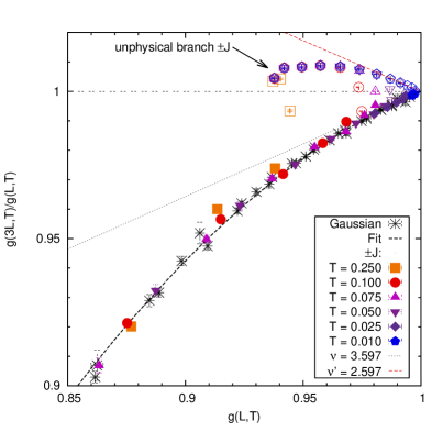
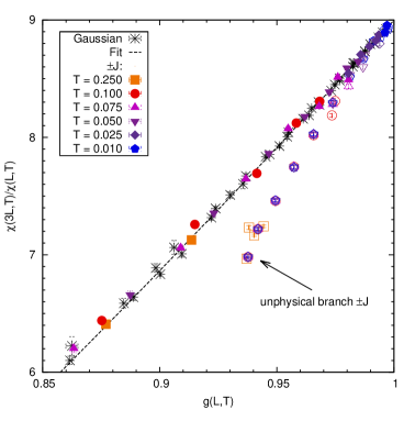
Figure 4: (Color online) In the left panel the scaling function of the Binder ratio $g(L,T)$ is shown for that Gaussian and $\pm J$ model. The data collapse shows that they share same scaling function and hence the same critical exponent $\nu$. In the right panel the scaling function of the spin-glass susceptibility $\chi$ is shown. The data collapse on the physical branch of the scaling functions shows that the critical exponent $\eta$ is universal.

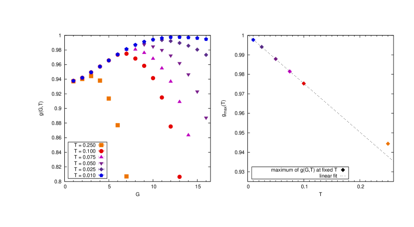
Figure 5: (Color online) In the left panel the Binder ratio $g(G,T)$ is shown as a function of the number of generations $G$ used in the construction of the hierarchical lattice. In the right panel the maximal value of the Binder ratio in shown as a function of temperature $T$. A linear extrapolation to zero temperature is very well compatible with universality, i.e., with $g_{c}=1$.

6 Discussion

Using the MKRG approach, we have studied 2D spin glasses, in particular the model with discrete couplings and its two different spin-glass phases at zero temperature. In the thermodynamic limit, one can observe each of these phases depending on how the zero-temperature limit is taken: If one takes first the zero-temperature limit (or simply sets the temperature to zero right from the beginning as it is often done in numerical ground state studies) and then sends the size to infinity, the discrete fixed point is obtained. If however, one first sends the size $L$ to infinity and then sends the temperature to zero, then entropy fluctuations (and temperature chaos) play a role and one is in fact observing a fixed point identical to the one reached with continuous couplings, strongly indicating that there is universality in 2D spin glasses. It is important to note that the physically relevant fixed point is the one which determines how quantities such as the spin-glass correlation length or the spin-glass susceptibility diverge as the temperature approaches the critical temperature $T_{c}=0$ and this is in all cases the continuous-coupling fixed point. It is also important to note that physically the domain-wall free-energy exponent is $\theta=1/\nu=-0.278$ also in the discrete coupling model if the thermodynamic limit is taken such that the system size is always kept larger than $l_{c}(T)$ which notably is not the case if one simply sets the temperature to zero in a finite-size scaling study (this leads to the well-known $\theta^{\prime}=0$.) At finite size, the observed properties depend on the length scale under probe and the crossovers between the different regimes are associated with the chaotic length scale $\ell_{c}$ and the paramagnetic one $L_{\rm eq}$.

The study of the continuous unstable fixed point is made difficult in simulations because of the cascade in the MKRG flow. However, we have shown that when using proper RG invariant quantities, one can measure the exponents associated with the fixed points precisely. Let us finally point out that this situation, where the entropy changes drastically the properties at zero temperature, is not entirely new. In fact, this is precisely the effect that changes the location of the spin-glass transition in diluted 3D spin glasses[14] from the naive percolation point to a nontrivial one: this shows how much entropic effects, and temperature chaos, matter in any renormalization or scaling scheme of finite-dimensional spin glasses [13]. In fact, such entropic effects also matter in mean-field spin glasses and optimization problems [33]. One has therefore always to be cautious in using ground-state properties if the entropy is not taken into account, because the presence of an additional unphysical fixed point might lead to wrong results.

During the (long) preparation of this manuscript, we became aware of the work of [15], who first stressed the role of temperature chaos. In fact the exponent $5.5$ they find in $2D$ is precisely $\nu_{\rm eff}$ in Table 2. The recent simulations of [12], as well as the older ones in [10], display strong indications supporting our analysis in 2D spin glasses on square lattices.

References

References

- [1] Y. Imry and S.-K. Ma. Random-Field Instability of the Ordered State of Continuous Symmetry. Phys. Rev. Lett., 35:1399, 1975.
- [2] S. F. Edwards and P. W. Anderson. Theory of spin glasses. J. Phys. F: Met. Phys., 5:965, 1975.
- [3] M. Mézard, G. Parisi, and M. A. Virasoro. Spin Glass Theory and Beyond. World Scientific, Singapore, 1987.
- [4] M. Mézard and A Montanari. Information, Physics and Computation. World Scientific, Oxford, 2010.
- [5] R. N. Bhatt and A. P. Young. Numerical studies of Ising spin glasses in two, three and four dimensions. Phys. Rev. B, 37:5606, 1988.
- [6] L. Saul and M. Kardar. Exact integer algorithm for the two-dimensional Ising spin glass. Phys. Rev. E, 48:R3221, 1993.
- [7] J. Houdayer. A cluster Monte Carlo algorithm for 2-dimensional spin glasses. Eur. Phys. J. B., 22:479, 2001.
- [8] A. K. Hartmann. Ground-state clusters of two-, three-, and four-dimensional Ising spin glasses. Phys. Rev. E, 63, 2001.
- [9] C. Amoruso, E. Marinari, O. C. Martin, and A. Pagnani. Scalings of Domain Wall Energies in Two Dimensional Ising Spin Glasses. Phys. Rev. Lett., 91:87201, 2003.
- [10] T. Jörg, J. Lukic, E. Marinari, and O. C. Martin. Strong Universality and Algebraic Scaling in Two-Dimensional Ising Spin Glasses. Phys. Rev. Lett., 96:237205, 2006.
- [11] J. Lukic, E. Marinari, O. C. Martin, and S Sabatini. Temperature chaos in two-dimensional Ising spin glasses with binary couplings: a further case for universality . J. Stat. Mech., page L10001, 2006.
- [12] F. P. Toldin, A. Pelissetto, and E. Vicari. Universality of the glassy transitions in the two-dimensional ±j ising model. Phys. Rev. E, 82:021106, 2010.
- [13] F. Krzakala and O. C. Martin. Discrete energy landscapes and replica symmetry breaking at zero temperature. Europhys. Lett., 53:749, 2001.
- [14] T. Jörg and F. Ricci-Tersenghi. Entropic Effects in the Very Low Temperature Regime of Diluted Ising Spin Glasses with Discrete Couplings. Phys. Rev. Lett., 100:177203, 2008.
- [15] K. T. Creighton, D. A. Huse, and A. A. Middleton. Chaos and universality in two-dimensional ising spin glasses. 2010. arXiv:1012.3444.
- [16] D. S. Fisher and D. A. Huse. Ordered phase of short-range Ising spin-glasses. Phys. Rev. Lett., 56:1601, 1986.
- [17] A. J. Bray and M. A. Moore. In L. Van Hemmen and I. Morgenstern, editors, Heidelberg Colloquium on Glassy Dynamics and Optimization. Springer, New York, 1986.
- [18] A. J. Bray and M. A. Moore. Chaotic Nature of the Spin-Glass Phase. Phys. Rev. Lett., 58:57, 1987.
- [19] Kadanoff, L.P. ”Statistical Physics: Statics, Dynamics and Renormalization”. World Scientific.
- [20] M. Ohzeki and H. Nishimori. Analytical evidence for the absence of spin glass transition on self-dual lattices. J. Phys. A, 42:332001, 2009.
- [21] B. W. Southern and A. P. Young. Real space rescaling study of spin glass behaviour in three dimensions . J. Phys. C, 10:2179, 1977.
- [22] K. H. Fisher and J. A. Hertz. Spin Glasses. Cambridge University Press, Cambridge, 1991.
- [23] G. Migliorini and A.N. Berker. Global random-field spin-glass phase diagrams in two and three dimensions. Phys. Rev. B, 57:426, 1998.
- [24] S. R. McKay, A. N. Berker, and S. Kirkpatrick. Spin-Glass Behavior in Frustrated Ising Models with Chaotic Renormalization-Group Trajectories. Phys. Rev. Lett., 48:767, 1982.
- [25] A. K. Hartmann, A .J. Bray, A. C. Carter, M. A. Moore, and A. P. Young. The stiffness exponent of two-dimensional Ising spin glasses for non-periodic boundary conditions using aspect-ratio scaling. Phys. Rev. B, 66:224401, 2002.
- [26] C. Amoruso, A. K. Hartmann, M. B. Hastings, and M. A. Moore. Conformal Invariance and SLE in Two-Dimensional Ising Spin Glasses. Phys. Rev. Lett., 97:267202, 2006.
- [27] Denis Bernard, Pierre Le Doussal, and A. Alan Middleton. Possible description of domain walls in two-dimensional spin glasses by stochastic loewner evolutions. Phys. Rev. B, 76(2):020403, Jul 2007.
- [28] O. Melchert and A. K. Hartmann. Fractal dimension of domain walls in two-dimensional ising spin glasses. Phys. Rev. B, 76(17):174411, Nov 2007.
- [29] F. Krzakala and O. C. Martin. Chaotic temperature dependence in a model of spin glasses. A random-energy random-entropy model. Eur. Phys. J. B, 28:199, 2002.
- [30] M. Nifle and H. J. Hilhorst. New critical-point exponent and new scaling laws for short-range Ising spin glasses. Phys. Rev. Lett., 68:2992, 1992.
- [31] T. Jörg and H. G. Katzgraber. Evidence for Universal Scaling in the Spin-Glass Phase. Phys. Rev. Lett., 101:197205, 2008.
- [32] M. A. Moore, H. Bokil, and B. Drossel. Evidence for the droplet picture of spin glasses. Phys. Rev. Lett., 81:4252, 1998.
- [33] F. Krza̧kała, A. Montanari, F. Ricci-Tersenghi, G. Semerjian, and L. Zdeborova. Gibbs states and the set of solutions of random constraint satisfaction problems. Proc. Nat. Am. Soc., 104:10318, 2007.