Super-Alfvénic propagation of reconnection signatures and Poynting flux during substorms

Abstract

The propagation of reconnection signatures and their associated energy are examined using kinetic particle-in-cell simulations and Cluster satellite observations. It is found that the quadrupolar out-of-plane magnetic field near the separatrices is associated with a kinetic Alfvén wave. For magnetotail parameters, the parallel propagation of this wave is super-Alfvénic $(V_{\parallel}\sim 1500-5500\,{\rm km/s})$ and generates substantial Poynting flux $(S\sim 10^{-5}-10^{-4}\,{\rm W/m^{2}})$ consistent with Cluster observations of magnetic reconnection. This Poynting flux substantially exceeds that due to frozen-in ion bulk outflows and is sufficient to generate white light aurora in the Earth’s ionosphere.

Magnetic reconnection plays an important role in many plasma systems by releasing large amounts of magnetic energy through the breaking and reforming of magnetic field lines (e.g., Yamada et al. (2010)). During magnetospheric substorms the global magnetic geometry is reconfiguredAkasofu (1964), releasing magnetotail magnetic energy and creating intense auroral disturbances. During solar flares, magnetic energy release in the corona energizes large numbers of electrons which create hard x-rays when they impact to surface of the sun (e.g., Miller et al. (1997)).

The sudden onset of magnetospheric substorms is believed to be caused by either a near Earth instability at around $10\,R_{e}$ downtail (e.g., Lui (1996)) or reconnection onset around $20$ to $30\,R_{e}$ (e.g., Baker et al. (1996)). Determining the mechanism or mechanisms which are most relevant requires careful timing studies and has been the subject of much scrutiny and controversy (e.g., Angelopoulos et al. (2008); Lui (2009); Angelopoulos et al. (2009); Kepko et al. (2009); Nishimura et al. (2010)). A key unanswered question regarding magnetic reconnection, therefore, regards how fast the released energy and associated signatures propagate away from the X-line. The propagation of MHD signatures, ion flows and magnetic disturbances, has been extensively studied in both substorms (e.g., Birn et al. (1999)) and solar flares (e.g., Linton and Longcope (2006)), but these mechanisms are limited by the Alfvén speed. In some substorm events, however, it has been reported that the time lag between reconnection onset and auroral onset was less than the Alfvén transit time from the reconnection site to the ionosphereAngelopoulos et al. (2008); Lin et al. (2009). It is necessary, therefore, to determine the nature of the reconnection signal that propagates fastest away from a reconnection site and its associated energies. Poynting fluxWygant et al. (2000); Keiling et al. (2003) associated with kinetic Alfvén waves, for example, has been postulated as a possible energy source for auroraLysak and Song (2004), with observations of these waves near magnetotail reconnection sitesChaston et al. (2009); Dai (2009).

We simulate magnetic reconnection with the kinetic particle-in-cell code P3D and find that the quadrupolar Hall out-of-plane magnetic field located near the separatrices is associated with a kinetic Alfvén wave (KAW). This KAW magnetic field perturbation has a super-Alfvénic parallel propagation speed (using lobe densities), and is associated with a substantial Poynting flux that points away from the X-line. This KAW will exist whenever Hall physics is active in the diffusion region Rogers et al. (2001). Simulation Poynting flux is consistent with Cluster statistical observations of multiple magnetotail reconnection events. Scaling to magnetotail and ionospheric parameters, the transit time of this standing KAW from a near Earth X-line is on the order of 50 seconds.

Simulations: Our simulations are performed with the particle-in-cell code p3d Zeiler et al. (2002). The results are presented in normalized units: the magnetic field to the asymptotic value of the reversed field $B_{0}$, the density ($n_{0}$) to the value at the center of the current sheet minus the uniform background density, velocities to the Alfvén speed $c_{A}$, lengths to the ion inertial length $d_{i}$, times to the inverse ion cyclotron frequency $\Omega_{ci}^{-1}$, temperatures to $m_{i}c_{A}^{2}$, and Poynting flux to $S_{0}=c_{A}\,B_{0}^{2}/4\pi$. We consider a system periodic in the $x-z$ plane where flow into and away from the X-line are parallel to $\mathbf{\hat{z}}$ and $\mathbf{\hat{x}}$, respectively. The initial equilibrium consists of two Harris current sheets superimposed on an ambient population with a uniform density of $0.2$. The equilibrium magnetic field is given by $B_{x}=\tanh[(y-L_{z}/4)/w_{0}]-\tanh[(y-3L_{z}/4)/w_{0}]-1$, where $w_{0}$ and $L_{z}$ are the half-width of the initial current sheets and the box size. The electron and ion temperatures, $T_{e}=1/12$ and $T_{i}=5/12$, are initially uniform. The simulations presented here are two-dimensional, i.e., $\partial/\partial y=0$. Reconnection is initiated with a small initial magnetic perturbation.

We have explored the separatrix structure and reconnection signal with three different simulations, varying the electron mass as shown in Table 1.

Table 1: Simulation parameters and results: $\Delta=$ grid scale, $c=$ light speed, $(L_{x},L_{z})$ = system size, $(\lambda,k,V_{sim},S_{sim})$ = properties of KAW. $(d_{i\ell},d_{e\ell})$ = lobe inertial lengths.

$\frac{m_{i}}{m_{e}}$	$\frac{\Delta}{d_{i}}$	$\frac{c}{c_{A}}$	$\frac{L_{x}}{d_{i}}$	$\frac{L_{z}}{d_{i}}$	$\frac{\lambda}{d_{i}}$	$k\,d_{i\ell}$	$k\,d_{e\ell}$	$\frac{V_{\par sim}}{c_{A}}$	$\frac{S_{\par sim}}{S_{0}}$
25	0.05	15	204.8	102.4	7.4	1.9	0.38	2.3	0.08
100	0.025	20	102.4	51.2	4.0	3.5	0.35	3.1	0.13
400	0.0125	40	51.2	25.6	2.6	5.4	0.27	4.0	0.18

These simulations were used for a previous study of reconnectionShay et al. (2007). As shown in Fig. 1 of citationShay et al. (2007) the reconnection rate increases with time, sometimes undergoes a modest overshoot, and approaches a quasi-steady rate of around $0.15$.

The structure of roughly one quadrant of the reconnection region is shown in Fig. 1, with the X-line located at $(x/d_{i},z/d_{i})=(21.36,6.40)$.

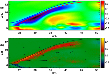
Figure 1: 2D overview plots. (a) $B_{y}$, with red and blue magnetic field line segments used in Fig. 2. (b) Parallel poynting flux ${\bf S}\cdot\hat{\bf b}_{xz}$ with ion velocity vectors. Black line is separatrix magnetic field line.

The large $B_{y}$ associated with Hall physics is clearly evident near the separatrix. This magnetic field is produced by nearly parallel electron flows near the separatrices, which are strongly super-Alfvénic. There is a strong Poynting flux parallel to the in-plane magnetic field, ${\bf S}\cdot\hat{\bf b}_{xz}$, where $\hat{\bf b}_{xz}=({\bf B}_{x}+{\bf B}_{z})/\sqrt{B_{x}^{2}+B_{z}^{2}}$. It is this Poynting flux which carries the energy of the first signal of reconnection. Note that there is little ion flow associated with this $B_{y}$ and Poynting flux.

In order to gain some handle on the physics governing this $B_{y}$ structure associated with reconnection, we represent it as a superposition of linear waves with various $k$ values. The scaling laws based on this analysis will be shown to be consistent with simulation properties. Examining Fig. 1a, the quasi-1D $B_{y}$ structure is very nearly parallel to the separatrix and thus is a strongly oblique wave with $k_{\parallel}\ll k_{\perp}$. As a starting point, we use the two-fluid analysis from previous studiesRogers et al. (2001); Drake et al. (2008), and analyze the branch of waves associated with Alfvén waves and kinetic Alfvén waves. For the simulation parameters used in this study and noting also that $kd_{e}\lesssim 1,$ with $d_{e}$ the electron skin depth:

$$\frac{\omega^{2}}{k_{\parallel}^{2}}=\frac{c_{A}^{2}}{D}\left[1+\left(\frac{k^{2}d_{i}^{2}}{D}\right)\frac{c_{s}^{2}}{c_{A}^{2}/D+c_{s}^{2}}\right],$$ (1)

with $D=1+k^{2}d_{e}^{2}$ and $c_{s}^{2}=(T_{e}+T_{i})/m_{i}.$ Note that for highly oblique waves, the parallel group velocity is equal to the parallel phase velocity.

Simulation KAW: This analysis uses quasi-steady reconnection to study the properties of the separatrix kinetic Alfvén wave (KAW). This is necessary because the KAW is so fast that the quadrupolar field associated with it very quickly fills the whole simulation domain making velocity measurements due to direct time variation impossible; the high speed of the KAW is most likely why its propagation velocities have been largely ignored by previous studies of collisionless reconnection, although other properties of the quadrupolar field have been extensively examined through simulations, satellite observations, and laboratory experiments (Yamada et al. (2010), and references therein). During steady reconnection, magnetic field lines convect along the inflow ($z$) direction, reconnect, and then flow outwards. The propagation velocity of the KAW can be measured by changing frames to one moving with that inflowing magnetic field line. Since the reconnection is steady, the time difference between two magnetic field lines is the difference in flux between the two lines over the reconnection rate, i.e., $\Delta t=\Delta\psi/E_{r}=$ $\Delta\psi/(\,\partial/\partial t(\psi_{\rm xline}-\psi_{\rm oline})\,),$ where $\psi$ is defined such that ${\bf B}=\hat{\bf y}\times\nabla\psi+B_{y}\,\hat{\bf y}$. By examining the KAW $B_{y}$ at different $\psi$ values, therefore, one can determine the propagation speed of the KAW. An example of this analysis for the $m_{e}/m_{i}=1/400$ case is shown in Fig. 2, which shows the variation of $B_{y}$ along magnetic field lines (lines of constant $\psi$).

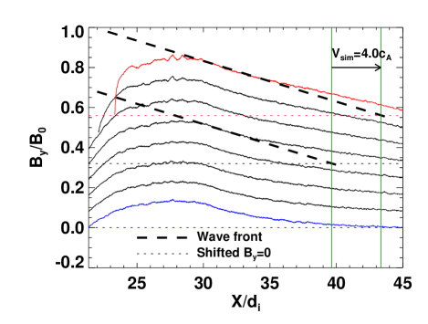
Figure 2: $B_{y}$ plotted along magnetic field lines separated by $\Delta\psi=0.05\,B_{0}d_{i},$ which represents $\Delta t=0.31\,\Omega_{ci}^{-1}$. Vertical offset of each plot is $0.08\,B_{0}$. Wave fronts for $\Delta\psi=0.2\,B_{0}d_{i}$ and $0.35\,B_{0}d_{i}$ shown as dashed lines, with respective $B_{y}=0$ shown as horizontal dotted lines. Blue and red $B_{y}$ plots taken along field line segments shown in Fig. 1a. Wave front intersections with $B_{y}=0$ denoted with vertical green lines.

For clarity, two representative magnetic field line segments colored red and blue are shown in Fig. 1a, and the $B_{y}$ plots taken along them are colored the same. Each $B_{y}$ plot represents a $\Delta\psi=0.05\,B_{0}d_{i}$, and each successive plot has been offset $0.08\,B_{0}$ along the vertical from the previous one. The evolution of the $B_{y}$ is not characterized by a simple propagation. First, the peak value of $B_{y}$ increases with time. Second, the dispersive nature of KAWs also leads to multiple velocities associated with the $B_{y}$ structure. The location where $B_{y}=0$ propagates at the peak KAW speed, $V_{\rm peak}\approx C_{se}=$ $\sqrt{(T_{e}+T_{i})/m_{e}}\approx 14\,c_{A}$. However, there is little Poynting flux associated with this velocity. Instead, we focus on the propagation of the main $B_{y}$ signal by finding the velocity of the wave front. The two dashed lines in Fig. 2 have the same slope and denote the wave front in two of the curves separated by $\Delta\psi=0.15\,B_{0}d_{i}.$ The propagation velocity of the x-intercept of this slope (shown as vertical green lines) is calculated to be $4.0\,c_{A},$ which is substantially less than the peak parallel KAW speed. The measured values are shown as $V_{sim}/c_{A}$ in Table 1.

It is critical to determine if this propagation velocity is consistent with the kinetic Alfven wave predictions of Eq. (1). First, the $k$ values associated with this $B_{y}$ Hall field must be determined. Vertical slices of the Poynting flux ${\bf S}\cdot\hat{\bf b}_{xz}$ were analyzed at the locations of the wave front ($m_{i}/m_{e}=[25,100,400]$, $x/d_{i}=[170.0,90.0,35.0]$). The magnitude of this Poynting flux is shown in Table 1 as $S_{sim}$. The width at half-max of the Poynting flux was measured and used to determine the primary $k=2\pi/\lambda$ value for the KAW. As an example, for the $m_{i}/m_{e}=400$ case, the half max was $\delta=0.65\,d_{i},$ yielding $\lambda\approx 2.6\,d_{i}$. The standing KAW wave is located close to the separatrices, so the simulation lobe plasma values are used to determine parameters ($B\approx 1.0,n\approx 0.2,T_{i}+T_{e}\approx 0.5$), which yields $kd_{i\ell}\approx 5.4,$ where the “$\ell$” denotes lobe values. The resulting $\lambda,kd_{i\ell},$ and $kd_{e\ell}$ are shown in Table 1. Plotting the velocities predicted from Eq. (1) versus the simulation measured velocities yields excellent agreement, as shown in Fig. 3a.

Figure 3: Simulation values versus theoretical predictions for (a) KAW propagation speed and (b) Poynting flux.

Associated with this Hall structure are electron beams and significant Poynting flux. The super-Alfvénic electron beams are associated with the parallel currents which create the quadrupolar $B_{y}$. A theoretical prediction for the Poynting flux can be determined for comparison with simulation values. We use ${\bf S}\cdot\hat{\bf b}_{xz}\approx S_{x}=(c/4\pi)({\bf E}\times{\bf B})_{x}\approx-(c/4\pi)E_{z}B_{y}$. The normal Hall electric field is due to the frozen-in electron flow, which dominates over the ion flow, giving $E_{z}\approx V_{ex}B_{y}/c\approx-J_{x}B_{y}/(nec)\approx-B_{y}B_{y}^{\prime}/(4\pi ne)$ with $B_{y}^{\prime}=\partial B_{y}/\partial z$. Substituting gives $S_{x}\approx B_{y}B_{y}^{\prime}\,c_{Ay}\,d_{i}/4\pi$, where $c_{Ay}=B_{y}/\sqrt{4\pi m_{i}n}$. Note that the integrated KAW Poynting flux is independent of the width of the KAW. As with the KAW velocity determination, $n$ is the lobe density with $B_{y}\approx 0.25$ consistent with simulation values. Comparison of the theoretical Poynting fluxes with simulation values also yields excellent agreement, as seen in Fig. 3b. Note that this KAW Poynting flux substantially exceeds the Poynting flux associated with the ion bulk flow away from the X-line: $S_{x,\,\rm ion}\approx c_{A}B_{z}^{2}/4\pi,$ since $B_{z}^{2}\approx 0.01\,B_{0}^{2}\ll B_{y}^{2}$.

Comparisons with Satellite Data: A statistical study of reconnection events has been performed previouslyEastwood et al. (2010), where magnetotail reconnection crossings with correlated Geocentric Solar Magnetospheric (GSM) $B_{z}$ and $V_{ix}$ reversals were selected. In that studyEastwood et al. (2010), comparisons with simulations were made by renormalizing data using magnetic fields just upstream of the separatrices ($B_{s}$) and densities in the ion outflow region ($n_{\rm out}$), yielding normalization velocity $\bar{c}_{A}=B_{s}/\sqrt{4\pi m_{i}n_{\rm out}}$ and Poynting flux $\bar{S}=\bar{c}_{A}\,B_{s}^{2}/4\pi.$ Using these normalizations, the Poynting flux from this Cluster data set is compared with data from the $m_{i}/m_{e}=25$ case. For the simulation data, the normalization values used were $B_{s}=0.8$ and $n_{\rm out}=0.2$. The simulation sub-region used was a rectangle roughly centered on the X-line with length approximately $35\,d_{i}$ and height approximately $13\,d_{i}$, using $n=0.2$. Fig. 4 shows this comparison, where only normalized $S_{x}/\bar{S}>0.02$ is plotted. Tailward $S_{x}/{\bar{S}}$ is shown in red and Earthward $S_{x}/\bar{S}$ is shown in black.

Figure 4: (a) Simulation and (b) Cluster Observations: Poynting flux $S_{x}/\bar{S}>0.02$ scatter plot in $(B_{x}/B_{s},V_{ix}/\bar{c}_{A})$ plane (red: Tailward $S_{x}/\bar{S}$, black: Earthward $S_{x}/\bar{S}$). Simulation values in (a) are smaller circles due to large number of data points. Normalizations described in text.

The bounds of the simulation and Cluster data are similar, being limited to $|V_{ix}|\lessapprox 0.7$ and $|B_{x}|\lessapprox 1.0$. The separatrix KAW structure is present in both plots in the region of large $B_{x}$ and nearly zero $V_{ix}$. Both datasets show a strong correlation in the sign of $V_{ix}$ and $S_{x},$ implying that the Poynting flux points away from the X-line. However, for small $V_{ix}$ and larger $B_{x}$ there is some anti-correlation which corresponds to ion flow towards the X-line just outside the separatrices. Both data sets show significant $S_{x}$ for small $|B_{x}|$ and larger negative $V_{ix}$, which is associated with the very long outflow jet of super-Alfvénic electrons seen in simulations with kinetic electronsShay et al. (2007); Karimabadi et al. (2007) and satellite observationsPhan et al. (2007). There is an asymmetry, however, in the satellite data along $V_{ix}$ not present in the simulations, with only negative (tailward) $S_{x}/\bar{S}$ having significant values for $B_{x}\approx 0$ and finite $V_{ix}$. Some possible explanations are: (1) In most of the events, the satellite was initially tailward of the X-line and then crossed to the Earthward side, so Earthward flows represent more developed X-lines. (2) The obstacle presented by the strong Earth’s dipole field could create back pressure and lead to outflow asymmetries at the X-line. Or (3) 3D effects lead to this asymmetry.

Predictions for the Magnetotail: The KAW associated with the quadrupolar $B_{y}$ propagates at a super-Alfvénic speed and carries significant Poynting flux. To assess its importance for the magnetosphere, we use the following typical parametersAngelopoulos et al. (2008): $B\approx 20\,{\rm nT},\,n\approx 0.1\,{\rm cm}^{-3},\,T_{e}\approx 300\,{\rm eV}$, and $T_{i}\approx 1\,{\rm keV}$. As the KAW propagates large distances in the magnetotail, it is quite probable that the $k$ associated with it will decrease owing to the dispersive nature of KAWs. Taking the simulation $kd_{e}\approx 0.3$ to be the maximum expected $k$, we take $kd_{i}\approx 1$ to be the minimum $k$ because at this $k$ the KAWs are no longer dispersive. As is found in the simulations, we use $B_{y}/B_{\rm lobe}\approx 0.25$. These values yield the following ranges of parameters associated with the KAW: $V_{\parallel}\sim 1500-5500\,{\rm km/s},$ $S\sim 0.7\cdot 10^{-5}-9\cdot 10^{-5}\,{\rm W/m^{2}}$. For an X-line located $20\,R_{e}$ downtail from the Earth, the predicted propagation time is $\Delta t\sim 25-85\,{\rm sec}$, which is substantially less than the Alfvén transit time $(\sim 250\,{\rm sec})$ for the same distance.

An important question remains as to whether this KAW energy will be able to propagate to the Earth’s ionosphere and create aurora. In the simulations (largest $L_{x}\approx 10\,R_{e}$ and $\Delta t\approx 50\,s$ using simulation lobe parameters), the KAW propagates all the way to the edge of the simulation, but the limited length scale as well of lack of a dipole geometry make exact estimation of the wave attenuation impossible. This is an important question currently under study. Assuming parallel propagation of the Poynting flux so that it stays on the same magnetic flux tube, the Poynting flux in the ionosphere $S_{\rm ion}$ would be: $S_{\rm ion}\sim(B_{\rm ion}/B_{\rm lobe})S_{\rm lobe}\sim 10^{3}\,S_{\rm lobe}$. Reducing this flux by a factor of ten as an estimate of attenuation yields: $S_{\rm ion}\sim 10^{2}\,S_{\rm lobe}\sim 0.7\cdot 10^{-3}-9\cdot 10^{-3}\,{\rm W/m^{2}}$, which is still on the order of or greater than the $10^{-3}\,{\rm W/m^{2}}=1\,{\rm ergs/cm^{2}s}$ necessary to create a white light aurora.

Acknowledgments This work was supported by NASA grant NNX08AM37G, NSF grant ATM-0645271, and the STFC grant ST/G00725X/1 at Imperial College London. Computations were carried out at the National Energy Research Scientific Computing Center. The authors thank V. Angelopoulos, A. T. Y. Lui, T. Nishimura, L. Lyons, L. Kepko, and R. Lysak for helpful discussions.

References

- Yamada et al. (2010) M. Yamada et al., Rev. Modern Phys. 82, 603 (2010).
- Akasofu (1964) S. I. Akasofu, Planet. Space Sci. 12, 273 (1964).
- Miller et al. (1997) J. A. Miller et al., J. Geophys. Res. 102, 14631 (1997).
- Lui (1996) A. T. Y. Lui, J. Geophys. Res. 101, 13067 (1996).
- Baker et al. (1996) D. N. Baker et al., J. Geophys. Res. 101, 12975 (1996).
- Angelopoulos et al. (2008) V. Angelopoulos et al., Science 321, 931 (2008).
- Lui (2009) A. T. Y. Lui, Science 324, 1391 (2009).
- Angelopoulos et al. (2009) V. Angelopoulos et al., Science 324, 1391 (2009).
- Kepko et al. (2009) L. Kepko et al., Geophys. Res. Lett. 36, 24104 (2009).
- Nishimura et al. (2010) Y. Nishimura et al., J. Geophys. Res. 115, 7222 (2010).
- Birn et al. (1999) J. Birn et al., J. Geophys. Res. 104, 19895 (1999).
- Linton and Longcope (2006) M. G. Linton and D. W. Longcope, ApJ 642, 1177 (2006).
- Lin et al. (2009) N. Lin et al., J. Geophys. Res. 114, 12204 (2009).
- Wygant et al. (2000) J. R. Wygant et al., J. Geophys. Res. 105, 18675 (2000).
- Keiling et al. (2003) A. Keiling et al., Science 299, 383 (2003).
- Lysak and Song (2004) R. L. Lysak and Y. Song, in Substorms 7: Proceedings of the 7th International Conference on Substorms, edited by T. Pulkinnen and N. Ganushkina (Finnish Meteorological Institute, 2004), p. 81.
- Chaston et al. (2009) C. C. Chaston et al., Phys. Rev. Lett. 102, 015001 (2009).
- Dai (2009) L. Dai, Ph.D. thesis, University of Minnesota (2009).
- Rogers et al. (2001) B. N. Rogers et al., Phys. Rev. Lett. 87, 195004 (2001).
- Zeiler et al. (2002) A. Zeiler et al., J. Geophys. Res. 107, 1230 (2002).
- Shay et al. (2007) M. A. Shay et al., Phys. Rev. Lett. 99, 155002 (2007).
- Drake et al. (2008) J. F. Drake et al., Phys. Plasmas 15, 042306 (2008).
- Eastwood et al. (2010) J. P. Eastwood et al., J. Geophys. Res. 115, A08215 (2010).
- Karimabadi et al. (2007) H. Karimabadi et al., Geophys. Res. Lett. 34, L13104, (2007).
- Phan et al. (2007) T. D. Phan et al., Phys. Rev. Lett. 99, 255002 (2007).