The Probability Distribution for Non-Gaussianity Estimators

Abstract

One of the principle efforts in cosmic microwave background (CMB) research is measurement of the parameter ${f_{\rm{nl}}}$ that quantifies the departure from Gaussianity in a large class of non-minimal inflationary (and other) models. Estimators for ${f_{\rm{nl}}}$ are composed of a sum of products of the temperatures in three different pixels in the CMB map. Since the number $\sim N_{\mathrm{pix}}^{2}$ of terms in this sum exceeds the number $N_{\mathrm{pix}}$ of measurements, these $\sim N_{\mathrm{pix}}^{2}$ terms cannot be statistically independent. Therefore, the central-limit theorem does not necessarily apply, and the probability distribution function (PDF) for the ${f_{\rm{nl}}}$ estimator does not necessarily approach a Gaussian distribution for $N_{\rm pix}\gg 1$. Although the variance of the estimators is known, the significance of a measurement of ${f_{\rm{nl}}}$ depends on knowledge of the full shape of its PDF. Here we use Monte Carlo realizations of CMB maps to determine the PDF for two minimum-variance estimators: the standard estimator, constructed under the null hypothesis (${f_{\rm{nl}}}=0$), and an improved estimator with a smaller variance for ${f_{\rm{nl}}}\neq 0$. While the PDF for the null-hypothesis estimator is very nearly Gaussian when the true value of ${f_{\rm{nl}}}$ is zero, the PDF becomes significantly non-Gaussian when ${f_{\rm{nl}}}\neq 0$. In this case we find that the PDF for the null-hypothesis estimator ${\widehat{f_{\rm{nl}}}}$ is skewed, with a long non-Gaussian tail at ${\widehat{f_{\rm{nl}}}}>|{f_{\rm{nl}}}|$ and less probability at ${\widehat{f_{\rm{nl}}}}<|{f_{\rm{nl}}}|$ than in the Gaussian case. We provide an analytic fit to these PDFs. On the other hand, we find that the PDF for the improved estimator is nearly Gaussian for observationally allowed values of ${f_{\rm{nl}}}$. We discuss briefly the implications for trispectrum (and other higher-order correlation) estimators.

I Introduction

The simplest single-field slow-roll inflation models predict that primordial perturbations should be nearly Gaussian inflation , but with predictably small departures from Gaussianity localmodel . This is often quantified through the non-Gaussianity parameter ${f_{\rm{nl}}}$ defined by Luo:1993xx ,

$$\Phi=\phi+{f_{\rm{nl}}}\left(\phi^{2}-\left\langle\phi^{2}\right\rangle\right),$$ (1)

where $\Phi$ is the gravitational potential and $\phi$ a Gaussian random field. Standard single-field slow-roll inflation predicts ${f_{\rm{nl}}}\ll 1$ for the primordial field (although nonlinear evolution of the density field may produce ${f_{\rm{nl}}}\sim 1$ at the time of recombination; see, e.g., Ref. Bartolo:2004if ). However, multi-field larger or curvaton curvaton models, or models with sharp features Wang:2000 or wiggles Hannestad:2009yx may produce larger values of ${f_{\rm{nl}}}$. Measurement of ${f_{\rm{nl}}}$ has thus become one of the primary goals of cosmic microwave background (CMB) and large-scale-structure (LSS) research. Current limits from the CMB/LSS are in the ballpark of $|{f_{\rm{nl}}}|\lesssim 100$ limits ; halos . The plot has thickened with a suggestion yadavdetection (not universally accepted) that WMAP data prefers (at the $2.8\sigma$ level) ${f_{\rm{nl}}}\neq 0$, with a best-fit value ${f_{\rm{nl}}}\simeq 35$. The Planck satellite :2011ah is expected to achieve a sensitivity of ${f_{\rm{nl}}}\sim 5$.

In this paper, we address the following question: What is the probability distribution function (PDF) $P({\widehat{f_{\rm{nl}}}})$ for an estimator ${\widehat{f_{\rm{nl}}}}$ that is constructed from a CMB map? If the PDF departs from the Gaussian distribution that is often assumed, then the 99.7% confidence level (C.L.) interval for ${f_{\rm{nl}}}$ may be different than three times the standard deviation for ${f_{\rm{nl}}}$. The interpretation of measurements thus requires knowledge of this PDF.

The question arises as the theory predicts not only the mean value of the estimator ${\widehat{f_{\rm{nl}}}}$, but it also makes a prediction for the detailed functional form of the PDF $P({\widehat{f_{\rm{nl}}}})$. The consistency of a given measurement of ${\widehat{f_{\rm{nl}}}}$ with a theoretical prediction for ${f_{\rm{nl}}}$ depends on knowledge of the shape of $P({\widehat{f_{\rm{nl}}}})$. Thus, for example, we often evaluate or forecast the standard error $\sigma_{{f_{\rm{nl}}}}$ with which a given measurement will recover the true value of ${f_{\rm{nl}}}$ and then simply assume that the error is Gaussian. If so, then with $\sigma_{{f_{\rm{nl}}}}=10$, for example, a measurement of ${\widehat{f_{\rm{nl}}}}=30$ would represent a $3\sigma$ departure from ${f_{\rm{nl}}}=0$ and a measurement ${\widehat{f_{\rm{nl}}}}=0$ would represent a $3\sigma$ departure fom ${f_{\rm{nl}}}=30$. However, if the PDF depends on the true value ${f_{\rm{nl}}}$, and if that distribution is non-Gaussian, then it may be that a measurement ${\widehat{f_{\rm{nl}}}}=30$ could be easily consistent with a true value ${f_{\rm{nl}}}=0$, while a measurement ${\widehat{f_{\rm{nl}}}}=0$ could be inconsistent with ${f_{\rm{nl}}}=30$ with a confidence greater than “$3\sigma$.” We will see below that something like this actually occurs with measurements of ${f_{\rm{nl}}}$.

This question is particularly important for measurements of non-Gaussianity (as opposed, for example, for the CMB power spectrum), because ${\widehat{f_{\rm{nl}}}}$ is a sum over products of three temperature measurements (unlike the power spectrum, which sums over squares of temperature measurements). Suppose the temperature is measured in $N_{\mathrm{pix}}$ pixels. There are then $\sim N_{\mathrm{pix}}^{2}$ terms in the ${f_{\rm{nl}}}$ estimator (after restrictions imposed by statistical isotropy). While these terms may have zero covariance, they are not statistically independent; there is no way to construct $N_{\mathrm{pix}}^{2}$ statistically independent quantities from $N_{\mathrm{pix}}$ measurements! The conditions required for the validity of the central-limit theorem are therefore not met, and $P({\widehat{f_{\rm{nl}}}})$ will not necessarily approach a Gaussian in the $N_{\mathrm{pix}}\gg 1$ limit.

The PDF can be obtained from Monte Carlo simulations, but the simulations are very computationally intensive (e.g., Ref. Elsner:2009md ). The number of Monte Carlo realizations is thus usually limited to the number, $\lesssim 1000$, required to determine a 99.7% C.L. detection or sometimes even fewer if it is just the variance that is being estimated. Although with only 1000 realizations Fig. 8 in Ref. Elsner:2009md shows hints of a non-Gaussian PDF, simulations done up until now do not include enough realizations to precisely map the functional form of $P({\widehat{f_{\rm{nl}}}})$. The number of realizations required to map ultimately the $4\sigma$, $5\sigma$, etc. ranges will be prohibitive, especially since the simulations will need to be re-run repeatedly to determine how the error ranges depend on cosmological parameters, instrument-noise properties, scanning strategies, etc., and they then must be run for multiple theoretical values ${f_{\rm{nl}}}$.

Work along these lines was begun in Ref. Creminelli:2006gc , wherein it was shown that the variance of the distribution $P({\widehat{f_{\rm{nl}}}})$ may have a strong dependence on the true underlying value of ${f_{\rm{nl}}}$. More precisely, they evaluated the variance of the estimator designed to have the minimum variance under the null hypothesis ${f_{\rm{nl}}}=0$ (which we refer to frequently below as the “null-hypothesis minimum-variance” estimator, or NHMV estimator), and showed that the variance of this NHMV estimator increases as ${f_{\rm{nl}}}^{2}$ increases. They then constructed an alternative estimator $\widehat{f_{nl}^{n}}$, which we call the CSZ estimator, which has a PDF with a variance that saturates the Cramer-Rao bound up to corrections of order ${f_{\rm{nl}}}^{2}$. Still, as we have argued above, the consistency of a hypothesis with a measurement requires full knowledge of the PDF of whatever estimator is used in the analysis.

To address these questions, we calculate the PDF for an ideal (no-noise) map to understand the irreducible PDF introduced simply by cosmic variance under the Sachs-Wolfe approximation and on a flat sky. We hope that lessons learned about $P({\widehat{f_{\rm{nl}}}})$ in this ideal case may help interpret and understand current/forthcoming results and assess the validity of full-experiment simulations.

We calculate these PDFs by using Monte Carlo realizations of numerous no-noise flat-sky CMB maps. The first order of business with a map will be to determine whether a given map is consistent or inconsistent with the null hypothesis ${f_{\rm{nl}}}=0$. Therefore, we first calculate the PDF that arises if ${f_{\rm{nl}}}$ does indeed vanish, for the NHMV estimator ${\widehat{f_{\rm{nl}}}}$, and we also calculate the PDF that arises if the true value of ${f_{\rm{nl}}}$ is nonzero. We provide an analytic fit for these PDFs in Eq. (III.2). If the evidence from such a measurement were to show that ${f_{\rm{nl}}}$ is nonzero, then the next step would be to apply the CSZ estimator $\widehat{f_{nl}^{n}}$ for ${f_{\rm{nl}}}\neq 0$ Creminelli:2006gc to obtain a more precise value for ${f_{\rm{nl}}}$ or to test consistency of the data with a specific nonzero value of ${f_{\rm{nl}}}$. We therefore follow by calculating the PDF for these improved non-null-hypothesis estimators.

We find that, besides having a variance that increases with ${f_{\rm{nl}}}^{2}$, the PDF of the NHMV can have a significantly non-Gaussian shape when ${f_{\rm{nl}}}\neq 0$ with a long non-Gaussian tail for ${\widehat{f_{\rm{nl}}}}>|{f_{\rm{nl}}}|$ and less probability at ${\widehat{f_{\rm{nl}}}}<|{f_{\rm{nl}}}|$ than in the Gaussian case. As an example, taking ${f_{\rm{nl}}}=100$ for an experiment which measures multipoles out to $l_{\rm max}=3000$ (such as Planck) and assuming a Gaussian PDF for the NHMV this experiment measures $74\leq{\widehat{f_{\rm{nl}}}}\leq 148$ at the 99.7% C.L.; the actual PDF shows that this experiment measures $68\leq{\widehat{f_{\rm{nl}}}}\leq 143$ at the 99.7% C.L. Applying the CSZ estimator to the data we find it has a PDF which is well approximated by a Gaussian with ${\widehat{f_{\rm{nl}}}}=100\pm 12.5$ at 99.7% C.L.

This paper is organized as follows. In Sec. II we construct the standard minimum-variance estimator ${\widehat{f_{\rm{nl}}}}$ under the null hypothesis ${f_{\rm{nl}}}=0$ and discuss why the PDF for this estimator is not necessarily Gaussian, even in the limit of a large number of pixels. In Sec. III.1 we use Monte Carlo calculations to evaluate the PDF $P({\widehat{f_{\rm{nl}}}}$) for this estimator if the null hypothesis is indeed valid, i.e., if ${f_{\rm{nl}}}$ is indeed zero. We find that the PDF in this ${f_{\rm{nl}}}=0$ case is well approximated by a Gaussian, for $N_{\mathrm{pix}}\gg 1$, even though the central-limit theorem does not apply. In Sec. III.2, we calculate the PDF assuming that the null hypothesis is not valid, i.e., if ${f_{\rm{nl}}}\neq 0$. We find the PDFs in this case can be highly non-Gaussian, skewed to large $|{\widehat{f_{\rm{nl}}}}|$, with long large-${\widehat{f_{\rm{nl}}}}$ non-Gaussian tails and less likelihood at ${\widehat{f_{\rm{nl}}}}\leq|{f_{\rm{nl}}}|$ relative to the Gaussian distribution of the same variance. We provide fitting formulas for the PDF as a function of the estimator ${\widehat{f_{\rm{nl}}}}$, the true value of ${f_{\rm{nl}}}$, and the maximum multipole moment ${l_{\mathrm{max}}}$ of the map. In Sec. IV we discuss the PDF of the CSZ estimator. We show that this estimator is well approximated by a Gaussian for values of ${f_{\rm{nl}}}$ still allowed by observations. In Sec. V we summarize and discuss some possible implications of the work for other bispectra and also for the trispectrum and other higher-order statistics. An Appendix discusses the computational techniques we used in order to perform our Monte Carlo simulations.

II Non-Gaussianity estimators

II.1 Formalism

We assume a flat sky to avoid the complications (e.g., spherical harmonics, Clebsch-Gordan coefficients, Wigner 3$j$ and 6$j$ symbols, etc.) associated with a spherical sky, and we further assume the Sachs-Wolfe limit. We denote the fractional temperature perturbation at position $\vec{\theta}$ on a flat sky by $T(\vec{\theta})$ and refer to it hereafter simply as the temperature.

The field $T(\vec{\theta})$ has a power spectrum $C_{l}$ given by

$$\left\langle T_{\vec{l}_{1}}T_{\vec{l}_{2}}\right\rangle=\Omega\delta_{\vec{l}_{1}+\vec{l}_{2},0}C_{l},$$ (2)

where $\Omega=4\pi f_{\mathrm{sky}}$ is the survey area (in steradian),

$$T_{\vec{l}}=\int\,d^{2}\vec{\theta}\,e^{-i\vec{l}\cdot\vec{\theta}}T(\vec{\theta})\simeq\frac{\Omega}{N_{\mathrm{pix}}}\sum_{\vec{\theta}}e^{-i\vec{l}\cdot\vec{\theta}}T(\vec{\theta}),$$ (3)

is the Fourier transform of $T(\vec{\theta})$, and $\delta_{\vec{l}_{1}+\vec{l}_{2},0}$ is a Kronecker delta that sets $\vec{l}_{1}=-\vec{l}_{2}$. The power spectrum for $T(\vec{\theta})$ is given by

$$C_{l}=\frac{2\pi A}{l^{2}},$$ (4)

where the amplitude, $A\simeq 10^{-10}$. The bispectrum $B(l_{1},l_{2},l_{3})$ is defined by

$$\left\langle T_{\vec{l}_{1}}T_{\vec{l}_{2}}T_{\vec{l}_{3}}\right\rangle=\Omega\delta_{\vec{l}_{1}+\vec{l}_{2}+\vec{l}_{3},0}B(l_{1},l_{2},l_{3}).$$ (5)

The Kronecker delta insures that the bispectrum is defined only for $\vec{l}_{1}+\vec{l}_{2}+\vec{l}_{3}=0$; i.e., only for triangles in Fourier space. Statistical isotropy then dictates that the bispectrum depends only on the magnitudes $l_{1}$, $l_{2}$, $l_{3}$ of the three sides of this Fourier triangle.

II.2 The null-hypothesis minimum-variance estimator

We now review how to construct the minimum-variance estimator for ${f_{\rm{nl}}}$ under the null hypothesis. This is the quantity that one would first determine from the data to check for consistency of the measurement with the null hypothesis ${f_{\rm{nl}}}=0$.

From Eq. (5), each triangle $\vec{l}_{1}+\vec{l}_{2}+\vec{l}_{3}=0$ gives an estimator,

$$({\widehat{{f_{\rm{nl}}}}})_{123}=\frac{T_{\vec{l}_{1}}T_{\vec{l}_{2}}T_{\vec{l}_{3}}}{\Omega B(l_{1},l_{2},l_{3})/{f_{\rm{nl}}}},$$ (6)

and under the null hypothesis this has a variance proportional to

$$\frac{\Omega^{3}C_{l_{1}}C_{l_{2}}C_{l_{3}}}{\left[\Omega B(l_{1},l_{2},l_{3})/{f_{\rm{nl}}}\right]^{2}}.$$ (7)

The null-hypothesis minimum-variance estimator is constructed by adding all of these estimators with inverse-variance weighting. It is Babich:2004yc ; Kamionkowski:2010me

$${\widehat{f_{\rm{nl}}}}\equiv\sigma_{{f_{\rm{nl}}}}^{2}\sum_{\vec{l}_{1}+\vec{l}_{2}+\vec{l}_{3}=0}\frac{T_{\vec{l}_{1}}T_{\vec{l}_{2}}T_{\vec{l}_{3}}B(l_{1},l_{2},l_{3})/{f_{\rm{nl}}}}{6\Omega^{2}C_{l_{1}}C_{l_{2}}C_{l_{3}}},$$ (8)

and it has inverse variance,

$$\sigma_{{f_{\rm{nl}}}}^{-2}=\sum_{\vec{l}_{1}+\vec{l}_{2}+\vec{l}_{3}=0}\frac{\left[B(l_{1},l_{2},l_{3})/{f_{\rm{nl}}}\right]^{2}}{6\Omega C_{l_{1}}C_{l_{2}}C_{l_{3}}}.$$ (9)

II.3 Non-gaussianity of the PDF

If the number of pixels in the CMB map is $N_{\mathrm{pix}}$, then there are also $N_{\mathrm{pix}}$ statistically independent $T_{\vec{l}}$. But there are a much larger number, $\propto N_{\rm pix}^{2}$, of triplets $T_{\vec{l}_{1}}T_{\vec{l}_{2}}T_{\vec{l}_{3}}$, included in the estimator [cf., Eq. (8)], and so the number of individual “data points” (i.e., triplets) used in the minimum-variance estimator scales like $N_{\rm pix}^{2}\gg N_{\rm pix}$. Since the number of terms included in the estimator is greater than the number of independently measured data points the standard central-limit theorem does not apply. Thus, we cannot assume that the PDF of the estimator will approach a Gaussian in the $N_{\rm pix}\to\infty$ limit.

This contrasts with the estimator $\widehat{C}_{l}\propto\sum|T_{\vec{l}}|^{2}$ of the power spectrum $C_{l}$. While the PDF for $\widehat{C}_{l}$ is not necessarily Gaussian (it has a $\chi_{2l+1}^{2}$ distribution), it is the sum of the squares of statistically independent quantities. The central-limit theorem therefore applies, and the distribution for $\widehat{C}_{l}$ does indeed approach a Gaussian for large $l$. The problems we address here for ${f_{\rm{nl}}}$ estimators parallel those discussed in the literature for the quadrupole moment $C_{2}$, as the distribution for quadrupole-moment estimators will be highly non-Gaussian and will also depend on the underlying theory (see, e.g., Ref. Efstathiou:2003tv ).

III The PDF of ${\widehat{f_{\rm{nl}}}}$ for the local model

We now restrict our attention to a family of non-Gaussian models in which the temperature $T(\vec{\theta})$ has a non-Gaussian component; i.e.,

$$T(\vec{\theta})=t(\vec{\theta})+3{f_{\rm{nl}}}\left\{[t(\vec{\theta})]^{2}-\left\langle[t(\vec{\theta})]^{2}\right\rangle\right\},$$ (10)

where $t(\theta)$ is a Gaussian random field with a power spectrum $C_{l}$ given in Eq. (4). To zero-th order in ${f_{\rm{nl}}}$, the power spectrum and correlation function for $T(\vec{\theta})$ are the same as those for $t(\vec{\theta})$. Note that $T(\vec{\theta})$ is, strictly speaking, the temperature fluctuation, so $\left\langle T(\vec{\theta})\right\rangle=0=T_{\vec{l}=0}$. The bispectrum for this model is

$$B(l_{1},l_{2},l_{3})=6{f_{\rm{nl}}}(C_{l_{1}}C_{l_{2}}+C_{l_{1}}C_{l_{3}}+C_{l_{2}}C_{l_{3}}).$$ (11)

The temperature Fourier coefficients can be written $T_{\vec{l}}=t_{\vec{l}}+{f_{\rm{nl}}}\delta t^{2}_{\vec{l}}$ with

$$\delta t^{2}_{\vec{l}} \equiv \frac{3}{\Omega}\sum_{\vec{l}^{\prime}}t_{\vec{l}-\vec{l}^{\prime}}t_{\vec{l}^{\prime}}.$$ (12)

Formally, the sum goes from $0<|\vec{l}^{\prime}|\leq\infty$, but for a finite-resolution map, the sum is truncated at some $l_{\rm max}$ such that the number of Fourier modes equals the number of data points.

We now proceed to evaluate $P({\widehat{f_{\rm{nl}}}};{f_{\rm{nl}}},{l_{\mathrm{max}}})$, the PDF that arises if the true value is ${f_{\rm{nl}}}$ for the NHMV estimator ${\widehat{f_{\rm{nl}}}}$ and for a map with ${l_{\mathrm{max}}}$. To do so, we generated large numbers of Monte Carlo realizations of maps according to Eq. (12), for some assumed value of ${f_{\rm{nl}}}$, and then applied the estimator in Eq. (8) to these maps. Each map is simulated in harmonic space from $l_{\rm min}=2$ up to a maximum multipole $l_{\rm max}$. In order to produce a large number of realizations we re-expressed the generation of maps and implementation of the estimator in terms of fast Fourier transforms as discussed in Appendix A.

III.1 The PDF of the null hypothesis minimum-variance estimator with ${f_{\rm{nl}}}=0$

First we consider the shape of $P({\widehat{f_{\rm{nl}}}};{f_{\rm{nl}}}=0,l_{\rm max})$, the PDF for the NHMV estimator in Eq. (8) applied to a purely Gaussian (${f_{\rm{nl}}}=0$) map. To do this we generated $10^{6}$ Gaussian realizations and applied the estimator in Eq. (8) to generate a histogram of values of ${\widehat{f_{\rm{nl}}}}$. From this histogram we determined $P({\widehat{f_{\rm{nl}}}};{f_{\rm{nl}}}=0,l_{\rm max})$ out to four times the root-variance, as shown in Fig 1.

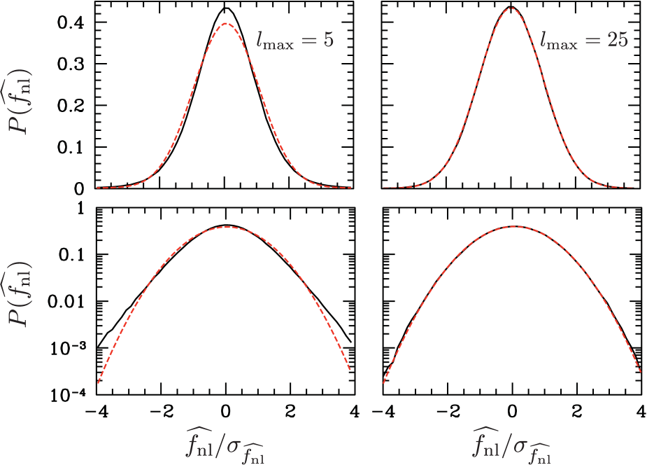
Figure 1: Numerical evaluations of $P({\widehat{f_{\rm{nl}}}};{f_{\rm{nl}}}=0,l_{\rm max})$. The left (right) two panels show the PDF for $l_{\rm max}=5$ and $l_{\rm max}=25$ for $10^{6}$ realizations for a scale-invariant power spectrum. In all panels the PDF has been normalized to have a unit variance, and the corresponding Gaussian PDF (with the same variance) is shown as the red dashed curve. As $l_{\rm max}$ gets larger, the PDF tends towards a Gaussian. This is not guaranteed by the central-limit theorem since the majority of the terms that appear in the estimator are not statistically independent.

First we note that our simulations verify that the variance of the distribution for the null case is well approximated by the analytic expression Babich:2004yc ; Kamionkowski:2010me ,

$$\sigma_{{f_{\rm{nl}}}}^{2} \approx \frac{1}{8Al_{\rm max}^{2}\ln(l_{\rm max})}.$$ (13)

Additionally our simulations show that out to at least four times the root-variance, the PDF $P({\widehat{f_{\rm{nl}}}};{f_{\rm{nl}}}=0,l_{\rm max})$ is well approximated by a Gaussian for $l_{\rm max}\gtrsim 25$, even though the conditions for the central-limit theorem to apply are not satisfied. Therefore, a measurement of ${\widehat{f_{\rm{nl}}}}$ that differed from 0 at more than three times the root-variance would indeed constitute a ‘99.7% confidence level’ inconsistency with the ${f_{\rm{nl}}}=0$ hypothesis.

III.2 The PDF of the null hypothesis minimum-variance estimator with ${f_{\rm{nl}}}\neq 0$

We now consider the form of $P({\widehat{f_{\rm{nl}}}};{f_{\rm{nl}}},l_{\rm max})$ when $f_{\rm nl}\neq 0$, the PDF for the null-hypothesis minimum-variance estimator if the null hypothesis is in fact not valid. In this case, the non-Gaussian statistics of the $T_{\vec{l}}$s impart some non-Gaussianity to the ${\widehat{f_{\rm{nl}}}}$ PDF.

In Fig. 2 we show $P({\widehat{f_{\rm{nl}}}};{f_{\rm{nl}}},l_{\rm max})$ calculated using $10^{6}$ realizations with ${f_{\rm{nl}}}=1500$ and $l_{\rm max}=25$. Clearly the PDF in this case is highly non-Gaussian.

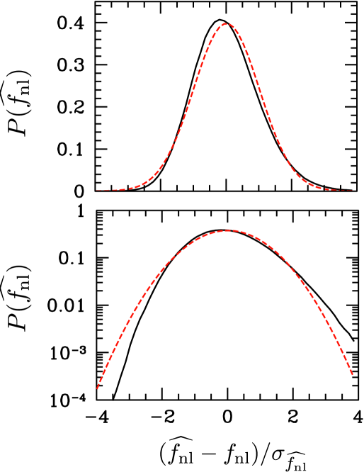
Figure 2: The PDF $P({\widehat{f_{\rm{nl}}}})$ when ${\widehat{f_{\rm{nl}}}}=1500$ using the estimator in Eq. (8) with $l_{\rm max}=25$. The upper (lower) panel shows the PDF on a linear (log) scale. We can see that the PDF is significantly non-Gaussian with an exponential drop-off to the left of mean and a power-law to the right. We provide a fitting formula for $P({\widehat{f_{\rm{nl}}}};{f_{\rm{nl}}},l_{\rm max})$ in the text.

Non-Gaussianity of $P({\widehat{f_{\rm{nl}}}};{f_{\rm{nl}}},l_{\rm max})$ for a central value ${f_{\rm{nl}}}\neq 0$ may be significant for the interpretation of data. Suppose, for example, that a CMB measurement returns ${\widehat{f_{\rm{nl}}}}=0$ with a root-variance $\sigma_{{f_{\rm{nl}}}}=40$. If the PDF was assumed to be Gaussian the measurement ${\widehat{f_{\rm{nl}}}}=0$ would rule out ${f_{\rm{nl}}}=100$ at the $2.5\sigma$ level, but given the asymmetric PDF of Fig. 2 it may rule out ${f_{\rm{nl}}}=100$ at a much higher significance.

In order to better understand the origin of the non-Gaussian PDF, it is useful to expand the minimum-variance estimator in Eq. (8) to linear order in ${f_{\rm{nl}}}$ Creminelli:2006gc :

$${\widehat{f_{\rm{nl}}}}\approx{E}_{0}+{f_{\rm{nl}}}{E}_{1}+\cdots,$$ (14)

where

$${E}_{0} = \sigma_{{f_{\rm{nl}}}}^{2}\sum_{\vec{l}_{1}+\vec{l}_{2}+\vec{l}_{3}=0}\frac{t_{\vec{l}_{1}}t_{\vec{l}_{2}}t_{\vec{l}_{3}}}{6\Omega^{2}{f_{\rm{nl}}}C_{l_{1}}C_{l_{2}}C_{l_{3}}}B(l_{1},l_{2},l_{3})$$ (15)

$${E}_{1} = \sigma_{{f_{\rm{nl}}}}^{2}\sum_{\vec{l}_{1}+\vec{l}_{2}+\vec{l}_{3}=0}\frac{\delta t^{2}_{\vec{l}_{1}}t_{\vec{l}_{2}}t_{\vec{l}_{3}}}{2\Omega^{3}C_{l_{1}}C_{l_{2}}C_{l_{3}}}B(l_{1},l_{2},l_{3}).$$ (16)

Since ${E}_{0}\sim t^{3}$ and ${E}_{1}\sim t^{4}$, it is clear that $\langle{E}_{0}\rangle=0$ and $\langle{E}_{0}{E}_{1}\rangle=0$, and the normalization guarantees that $\left\langle{E}_{1}\right\rangle=1$. Furthermore, since we have already established that $P({\widehat{f_{\rm{nl}}}})$ approaches a Gaussian in the large $l_{\rm max}$ limit if ${f_{\rm{nl}}}=0$, we know that, to leading order, the non-Gaussian shape of $P({\widehat{f_{\rm{nl}}}};{f_{\rm{nl}}},l_{\rm max})$ for ${f_{\rm{nl}}}\neq 0$ is being generated by ${E}_{1}$.

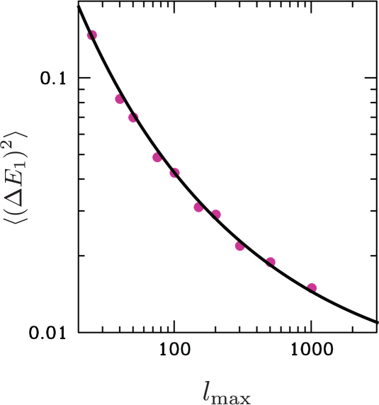
Figure 3: The dependence of $\left\langle(\Delta{E}_{1})^{2}\right\rangle$ on $l_{\rm max}$. The points correspond to the results of our Monte Carlo simulations for 1000 realizations at different values of $l_{\rm max}$. The solid curve shows the analytic calculation of the variance presented in Appendix B which is well-fit by the function $\left\langle(\Delta{E}_{1})^{2}\right\rangle=[14.0(l_{\rm max})^{0.433}]/[\ln^{5.1}(l_{\rm max})]\approx 4.5\ln^{-3}(l_{\rm max})$.

Some of the statistics associated with ${E}_{1}$ have already been explored in Ref. Creminelli:2006gc . There it is noted that the variance of ${\widehat{f_{\rm{nl}}}}$ is dominated by ${E}_{1}$ in the high $S/N$ limit leading to a slower scaling of the $S/N$ than the $l_{\rm max}^{-2}\ln^{-1}(l_{\rm max})$ scaling expected if the estimator saturated the Cramer-Rao bound Creminelli:2006gc . We explored the same limit using our Monte Carlo realizations, as shown in Fig. 3, and find the same qualitative trend but with a different dependence on $l_{\rm max}$. Ref. Creminelli:2006gc found $\langle(\Delta{E}_{1})^{2}\rangle\propto\ln^{-2}(l_{\rm max})$ whereas our simulations show $\langle(\Delta{E}_{1})^{2}\rangle\propto\ln^{-3}(l_{\rm max})$. We have checked the scaling found with our simulations by computing the variance analytically, as we further discuss in Appendix B. Fig. 3 shows the agreement between our analytic calculation (solid curve) and simulations (data points).

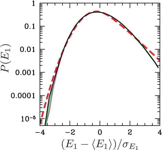
Figure 4: The PDF of ${E}_{1}$ calculated using $10^{6}$ realizations. The thin solid curves correspond to $P({E}_{1})$ with $l_{\rm max}=25$ (green), $l_{\rm max}=50$ (purple), $l_{\rm max}=100$ (black). Since the functional form of the PDF for each choice of $l_{\rm max}$ is nearly identical, we conclude that $P({E}_{1})$ approaches an asymptotic functional form in the large-$l_{\rm max}$ limit. The thick red dashed curve corresponds to a fit to $P({E}_{1})$, accurate to $\sim$10% out to 3 times the root variance, using the fitting formula in Eq. (17) with parameter values $x_{p}=-0.22$, $\sigma=0.80$, and $c=0.91$.

Our simulations allow us to generate the full PDF for $E_{1}$, not just the variance. Fig. 4 shows this PDF for various choices of $l_{\rm max}$ (thin solid lines). An important conclusion from Fig. 4 is that the shape of the PDF approaches a universal form in the $l_{\rm max}\gg 1$ limit. We provide a fit to the PDF (thick red dashed line), accurate to $\sim$10% (40%) out to three (four) times the root variance, using the fitting formula

$$\log[F(x)]=N-$$ (17)

$$\begin{cases}-(x-x_{p})^{2}/(2\sigma^{2}),&x\leq x_{p}\\ -\frac{c}{\sigma^{2}}\left(\sqrt{(x-x_{p})^{2}+c^{2}}-c\right),&x>x_{p},\end{cases}$$

where $N\equiv\sqrt{2/\pi}\sigma+c\exp[c^{2}/\sigma^{2}]K_{1}(c^{2}/\sigma^{2})$ and $K_{1}(x)$ is a modified Bessel function of the first kind, $c$ quantifies the non-Gaussianity of the distribution (and approaches a Gaussian in the $c\rightarrow\infty$ limit) and $x_{p}$ is the value of $(E_{1}-\left\langle E_{1}\right\rangle)/\sigma_{E_{1}}$ at the peak of the distribution. The red curve in Fig. 4 shows Eq. (17) with parameter values $x_{p}=-0.22$, $\sigma=0.80$, and $c=0.91$.

We are now in a position to write down a semi-analytic expression for $P({\widehat{f_{\rm{nl}}}};{f_{\rm{nl}}},l_{\rm max})$, accurate to $\sim$10% (40%) out to three (four) times the root variance, as a function of ${f_{\rm{nl}}}$ and $l_{\rm max}$. Letting $\sigma_{0}$ and $\sigma_{1}$ denote the standard deviations of the distributions for ${E}_{0}$ and ${E}_{1}$ respectively we have

$$\sigma_{0}^{2} \approx \frac{1}{8Al_{\rm max}^{2}\ln(l_{\rm max})},$$ (18)

$$\sigma_{1}^{2} \approx \frac{9{f_{\rm{nl}}}^{2}}{2\ln^{3}(l_{\rm max})}.$$ (19)

A good approximation to the PDF of ${\widehat{f_{\rm{nl}}}}$ is provided by the convolution of the PDF of ${E}_{0}$ and ${f_{\rm{nl}}}{E}_{1}$:

$$P({\widehat{f_{\rm{nl}}}};{f_{\rm{nl}}},l_{\rm max}) \approx \frac{4}{9\sqrt{2\pi}\sigma_{0}\sigma_{1}}$$

$$\times \int_{-\infty}^{\infty}G_{0}({\widehat{f_{\rm{nl}}}}-x)F([x-{f_{\rm{nl}}}]/\sigma_{1})dx,$$

where $G_{0}(x)$ is a Gaussian with zero mean and standard deviation $\sigma_{0}$ and $F([x-{f_{\rm{nl}}}]/\sigma_{1})$ is given by Eq. (17) with $x_{p}=-0.22$, $\sigma=0.80$, and $c=0.91$.

To obtain an analytic expression for the PDF we can approximate the convolution in Eq. (III.2) to write

$$P({\widehat{f_{\rm{nl}}}};{f_{\rm{nl}}},l_{\rm max})\approx\frac{2}{9}\exp\left[-\frac{X^{2}}{2(\sigma_{0}^{2}+\sigma_{1}^{2}\sigma^{2})}\right]\sqrt{\frac{1}{\sigma_{1}^{2}(\sigma_{0}^{2}+\sigma_{1}^{2}\sigma^{2})}}\Bigg{\{}\sigma_{1}\sigma\left(1+{\rm erf}\left[\frac{\sigma_{0}^{2}+\sigma_{1}\sigma^{2}(X+\sigma_{1})}{\sigma_{0}\sigma\sqrt{2(\sigma_{0}^{2}+\sigma_{1}^{2}\sigma^{2})}}\right]\right)$$

$$+ \sqrt{\sigma_{0}^{2}+\sigma_{1}^{2}\sigma^{2}}\left(1-{\rm erf}\left[\frac{c\sigma_{0}^{2}+\sigma_{1}\sigma^{2}(X+\sigma_{1})}{\sqrt{2}\sigma_{0}\sigma_{1}\sigma^{2}}\right]\right)\exp\left[\frac{1}{2}\left(\frac{c^{2}\sigma_{0}^{2}}{\sigma_{1}^{2}\sigma^{4}}+\frac{2c[X+\sigma_{1}c^{2}]}{\sigma_{1}\sigma^{2}}+\frac{X^{2}}{\sigma_{0}^{2}+\sigma_{1}^{2}\sigma^{2}}\right)\right]\Bigg{\}},$$

where $X\equiv{f_{\rm{nl}}}+x_{p}\sigma_{1}-\widehat{{f_{\rm{nl}}}}$.

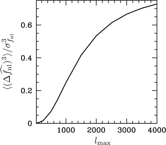
Figure 5: The skewness, $\langle(\Delta{\widehat{f_{\rm{nl}}}})^{3}\rangle$, as a fraction of the variance of $P({\widehat{f_{\rm{nl}}}};{f_{\rm{nl}}},l_{\rm max})$ as a function of $l_{\rm max}$ for ${f_{\rm{nl}}}=100$. We provide an analytic fitting formula in Eqs. (III.2) and (23) as a function of ${f_{\rm{nl}}}$ and $l_{\rm max}$.

Another useful way of quantifying the non-Gaussian shape of $P({\widehat{f_{\rm{nl}}}};{f_{\rm{nl}}},l_{\rm max})$ is to measure its skewness, $\langle(\Delta{\widehat{f_{\rm{nl}}}})^{3}\rangle$, as a function of ${f_{\rm{nl}}}$ and $l_{\rm max}$. We show this in Fig. 5 for ${f_{\rm{nl}}}=100$. An analytic fit to the skewness is given by

$$\frac{\langle(\Delta{\widehat{f_{\rm{nl}}}})^{3}\rangle}{\sigma_{{f_{\rm{nl}}}}^{3}}=\left(\frac{{f_{\rm{nl}}}}{100}\right)^{3}$$

$$\times \left(\frac{1}{1+3.7\exp\left[-(l_{\rm max}-5.1)/740\right]}-0.26\right),$$

with the variance of the distribution, $\sigma_{{f_{\rm{nl}}}}^{2}$, given by

$$\sigma_{{f_{\rm{nl}}}}^{2}\approx\frac{1}{8Al_{\rm max}^{2}\ln(l_{\rm max})}\left[1+\frac{36A{f_{\rm{nl}}}^{2}l_{\rm max}^{2}}{\ln^{2}(l_{\rm max})}\right].$$ (23)

Finally, we note that the shape of $P({\widehat{f_{\rm{nl}}}};{f_{\rm{nl}}},l_{\rm max})$ departs significantly from a Gaussian when $\sigma_{0}\simeq\sigma_{1}$. This occurs when

$${f_{\rm{nl}}}A^{1/2}\gtrsim\frac{\ln(l_{\rm max})}{6l_{\rm max}}.$$ (24)

Therefore, for the Planck satellite (i.e., $l_{\rm max}=3000$) the non-Gaussian features of $P({\widehat{f_{\rm{nl}}}};{f_{\rm{nl}}},l_{\rm max})$ for the NHMV estimator are significant if ${f_{\rm{nl}}}\gtrsim\mathcal{O}(10)$. Thus, given that Planck is expected to measure ${f_{\rm{nl}}}$ with a variance $\sigma\approx 5$, these PDFs may need to be taken into account to assign a precise confidence region with Planck data.

IV The PDF of an improved estimator when ${f_{\rm{nl}}}\neq 0$

As we saw in the previous Section the standard (null-hypothesis) minimum-variance estimator ${\widehat{f_{\rm{nl}}}}$ is constructed under the null hypothesis, so its variance is strictly minimized only when applied to maps with ${f_{\rm{nl}}}=0$ Creminelli:2006gc . In particular, the variance of ${\widehat{f_{\rm{nl}}}}$ is given in Eq. (23) so that when $36A{f_{\rm{nl}}}^{2}l_{\rm max}^{2}/\ln^{2}(l_{\rm max})\gtrsim 1$, the variance scales as the $\ln^{-3}(l_{\rm max})$, as opposed to $l^{-2}_{\rm max}\ln^{-1}(l_{\rm max})$. This indicates that when ${f_{\rm{nl}}}\neq 0$ there may be other estimators with smaller variances.

For a flat-sky and under the Sachs-Wolfe approximation Ref. Creminelli:2006gc introduced an improved estimator for ${f_{\rm{nl}}}\neq 0$ which has a variance that continues to decrease as $1/[l_{\rm max}^{2}\ln(l_{\rm max})]$ in the high signal-to-noise limit. To achieve this scaling they introduced a realization-dependent normalization,

$$\mathcal{N}\equiv\sigma_{{f_{\rm{nl}}}}^{2}\sum_{\vec{l}_{1}+\vec{l}_{2}+\vec{l}_{3}=0}\frac{\chi_{\vec{l}_{1}}T_{\vec{l}_{2}}T_{\vec{l}_{3}}}{2C_{l_{1}}C_{l_{2}}C_{l_{3}}}B(l_{1},l_{2},l_{3}),$$ (25)

where

$$\chi_{\vec{l}} \equiv \sum_{\vec{k}}T_{\vec{l}-\vec{k}}T_{\vec{k}}.$$ (26)

By construction $\left\langle\mathcal{N}\right\rangle=1$. They then define a new estimator constructed under the non-null hypothesis:

$$\widehat{f_{nl}^{n}}\equiv\frac{{\widehat{f_{\rm{nl}}}}}{\mathcal{N}}.$$ (27)

To explore the properties of the PDF of $\widehat{f_{nl}^{n}}$, we expand the normalization as $\mathcal{N}\approx\mathcal{N}_{0}+{f_{\rm{nl}}}\mathcal{N}_{1}+\cdots$ and write

$$\widehat{f_{nl}^{n}} \approx \frac{{E}_{0}}{\mathcal{N}_{0}}+{f_{\rm{nl}}}\frac{{E}_{1}\mathcal{N}_{0}-{E}_{0}\mathcal{N}_{1}}{\mathcal{N}_{0}^{2}}+\cdots,$$ (28)

$$\equiv \mathcal{E}_{0}+{f_{\rm{nl}}}\mathcal{E}_{1}+\cdots.$$ (29)

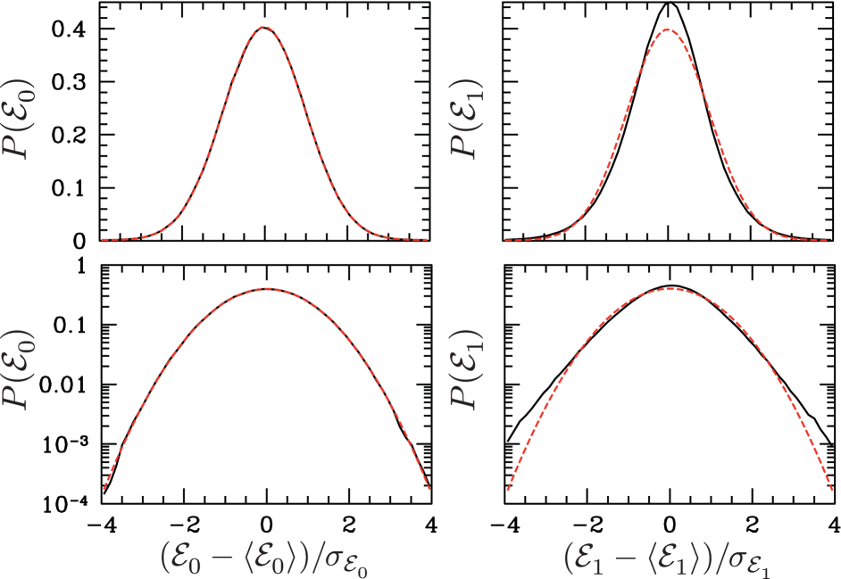
Figure 6: The PDF $P(\mathcal{E}_{0})$ (left) and $P(\mathcal{E}_{1})$ (right) for $l_{\rm max}=25$ determined with $10^{6}$ non-Gaussian realizations. The top panels show the PDF on a linear scale; the bottom panels show the PDF on a log scale. We have confirmed that the shape of the PDF is unchanged for larger values of $l_{\rm max}$. The PDF of $\mathcal{E}_{0}$ (left) is well approximated by a Gaussian. However, the PDF of the first-order correction $\mathcal{E}_{1}$ (right) has significant non-Gaussian wings. This implies that the full PDF of $\widehat{f_{nl}^{n}}$ is also non-Gaussian, even if the true value of ${f_{\rm{nl}}}$ matches that assumed in the construction of the CSZ estimator. Quantitatively, however, the level of non-Gaussianty will be small for Planck, as the variance of $\mathcal{E}_{1}$ is $\left\langle(\Delta\mathcal{E}_{1})^{2}\right\rangle\approx 9\ln^{2}(l_{\rm max})/(l_{\rm max}^{3})$.

In order to determine the shape of $P(\widehat{f_{nl}^{n}})$, we computed $P(\mathcal{E}_{0})$ and $P(\mathcal{E}_{1})$ for various values of $l_{\rm max}$. We found, as in the ${\widehat{f_{\rm{nl}}}}$ case, that these PDFs approach asymptotic shapes in the $l_{\rm max}\gg 1$ limit. We show these PDFs in Fig. 6 determined by $10^{6}$ realizations for $l_{\rm max}=25$. It is clear that $P(\mathcal{E}_{0})$ is very well approximated by a Gaussian, whereas $P(\mathcal{E}_{1})$ has significant non-Gaussian wings. As in the $P({\widehat{f_{\rm{nl}}}})$ case, this implies that the level of non-Gaussianity in $P(\widehat{f_{nl}^{n}})$ is significant only when the ratio ${f_{\rm{nl}}}^{2}\left\langle(\Delta\mathcal{E}_{1})^{2}\right\rangle/\left\langle(\Delta\mathcal{E}_{0})^{2}\right\rangle\gtrsim 1$. Our simulations show

$$\left\langle(\Delta\mathcal{E}_{0})^{2}\right\rangle \approx \frac{1}{8Al_{\rm max}^{2}\ln(l_{\rm max})},$$ (30)

$$\left\langle(\Delta\mathcal{E}_{1})^{2}\right\rangle \approx 9\frac{\ln^{2}(l_{\rm max})}{l_{\rm max}^{3}},$$ (31)

so that the PDF will be significantly non-Gaussian when

$${f_{\rm{nl}}}A^{1/2}\gtrsim\frac{1}{3}\left[\frac{l_{\rm max}}{8\ln(l_{\rm max})}\right]^{1/2}.$$ (32)

Therefore, for Planck (with $l_{\rm max}=3000$) $P(\widehat{f_{nl}^{n}};{f_{\rm{nl}}},l_{\rm max})$ will be significantly non-Gaussian only if ${f_{\rm{nl}}}\gtrsim\mathcal{O}(1000)$. Since this has already been ruled out by observations limits ; halos , we conclude that $P(\widehat{f_{nl}^{n}};{f_{\rm{nl}}},{l_{\mathrm{max}}})$ will be effectively Gaussian.

V Discussion

Here we have argued that the PDF for non-Gaussianity estimators cannot be assumed to be Gaussian, since the number of triplets used to construct these estimators may greatly exceed the number $N_{\mathrm{pix}}$ of measurements. The 99.7% confidence-level interval cannot safely be assumed to be 3 times the 66.5% confidence-level interval. We found, however, that the standard minimum-variance estimator ${\widehat{f_{\rm{nl}}}}$ constructed under the null hypothesis is well-approximated by a Gaussian distribution in the $l_{\rm max}\gg 1$ limit if the null hypothesis is correct (i.e., when applied to purely Gaussian maps).

We then calculated the same PDF $P({\widehat{f_{\rm{nl}}}})$ under the hypothesis that the true value of ${f_{\rm{nl}}}$ is non-zero. We find that the PDF is non-Gaussian in this case, skewed to large ${\widehat{f_{\rm{nl}}}}$ if ${f_{\rm{nl}}}>0$ and vice versa for ${f_{\rm{nl}}}<0$. The PDF for small positive or for negative ${\widehat{f_{\rm{nl}}}}$ is significantly smaller for ${f_{\rm{nl}}}>0$ than the Gaussian PDF with the same variance. Thus, for example, if the NHMV estimator gives ${\widehat{f_{\rm{nl}}}}>0$, it may actually rule out ${f_{\rm{nl}}}=0$ with a smaller statistical significance than would be inferred assuming a Gaussian distribution of the same variance. For Planck (with $l_{\rm max}\simeq 3000$) we find that the non-Gaussian shape of $P({\widehat{f_{\rm{nl}}}})$ is significant if ${f_{\rm{nl}}}\gtrsim\mathcal{O}(10)$. Thus, the non-Gaussian shape of the PDF may need to be taken into account, even in case of a null result, to assign a precise 99.7% confidence-level upper (or lower, for ${f_{\rm{nl}}}<0$) limit to ${f_{\rm{nl}}}$. We also provide, in Eq. (III.2), an analytic fit to these PDFs.

The non-Gaussian shape of $P({\widehat{f_{\rm{nl}}}})$ when ${f_{\rm{nl}}}\neq 0$ is accompanied by a variance that decreases only logarithmically with increasing $l_{\rm max}$. Because of this, Ref. Creminelli:2006gc constructed an improved estimator under the ${f_{\rm{nl}}}\neq 0$ hypothesis with a variance that saturates the Cramer-Rao bound and continues to decrease as $1/[l_{\rm max}^{2}\log(l_{\rm max})]$. We found that for observationally allowed values of ${f_{\rm{nl}}}$ this improved estimator has a PDF that is well approximated by a Gaussian shape. However, this estimator has only been defined under the Sachs-Wolfe limit and it is not immediately clear how it should be generalized to be applied to actual data. An alternative, Bayesian, approach to measuring ${f_{\rm{nl}}}$ which also saturates the Cramer-Rao bound in the presence of ${f_{\rm{nl}}}\neq 0$ is presented in Ref. Elsner:2010hb .

We have restricted our attention to the bispectrum in the local model, but the PDF must be similarly determined for the non-Gaussianity parameter for bispectra with other shape dependences; e.g., the equilateral model dvali ; Equil or that which arises with self-ordering scalar fields Figueroa:2010zx . It should also be interesting to explore the PDF for maximum-likelihood, rather than quadratic, estimators (see, e.g., Ref. Creminelli:2006gc ). Ultimately, a variety of experimental effects and more precise power spectra and bispectra, rather than the Sachs-Wolfe-limit quantities used here, will need to be included in interpreting the results of realistic experiments.

There is also interest in using higher-order correlation functions to measure ${f_{\rm{nl}}}$ from CMB maps. Our arguments should apply also to these higher-order correlation functions, like the trispectrum, etc. For example, the estimator for the amplitude of the $n$-point correlation function (e.g., $n=3$ for the bispectrum, $n=4$ for the trispectrum, etc.), will be constructed from $\sim N_{\mathrm{pix}}^{(n-1)}/n!$ combinations of $n$ pixels, and this number of combinations scales even more rapidly with $N_{\mathrm{pix}}$ than that for the bispectrum. Thus, although the signal-to-noise scales more rapidly with $N_{\mathrm{pix}}$ for these higher-order correlation functions than that for the bispectrum Kogo:2006kh ; Smidt:2010sv ; Kamionkowski:2010me , concerns about the PDF for these estimators should be even more serious than for the bispectrum. It will thus be necessary to understand the PDF for these higher-order estimators to confidently forecast the statistical signficance of measurements inprep .

Appendix A Computing non-Gaussianity estimators using FFTs

We are interested in using Monte Carlo simulations to determine the shape of the PDF of ${\widehat{{f_{\rm{nl}}}}}$ as a function of the fiducial choice of ${f_{\rm{nl}}}$ and the number $N_{\mathrm{pix}}$ of pixels measured in a given observation. Applying the estimator in Eq. (8) to the local-model bispectrum [Eq. (11)] it can be rewritten

$${\widehat{{f_{\rm{nl}}}}}=\sigma_{{f_{\rm{nl}}}}^{2}\sum_{|\vec{l}_{1}+\vec{l}_{2}+\vec{l}_{3}|=0}\frac{T_{\vec{l}_{1}}T_{\vec{l}_{2}}T_{\vec{l}_{3}}}{\Omega^{2}C_{l_{3}}}.$$ (33)

The estimator in Eq. (33) takes $N_{\mathrm{pix}}^{2}$ operations to evaluate. Since current CMB observations have $N_{\mathrm{pix}}\sim 10^{6}$ this estimator would take a prohibitively long time to evaluate for a significant number of realizations, especially since we are interested in probing the shape of the PDF far into the tail of the distribution ($\sim 3-4\sigma$).

As discussed at length in Ref. Komatsu:2003iq this is even more of a problem when measuring non-Gaussianity on the full sky where the number of operations scales as $N_{\mathrm{pix}}^{5/2}$. In order to make the problem tractable Ref. Komatsu:2003iq rewrites ${\widehat{{f_{\rm{nl}}}}}$ in terms of real-space quantities reducing the number of operations to $N_{\mathrm{pix}}^{3/2}$.

We can do the same for ${\widehat{{f_{\rm{nl}}}}}$ in the flat-sky approximation. Noting that

$$\delta_{\vec{l}_{1}+\vec{l}_{2}+\vec{l}_{3},0}=\int\frac{d^{2}\theta}{\Omega}e^{i\vec{\theta}\cdot(\vec{l}_{1}+\vec{l}_{2}+\vec{l}_{3})},$$ (34)

and writing

$$A(\vec{\theta}) \equiv \frac{1}{\Omega}\sum_{\vec{l}}e^{i\vec{l}\cdot\vec{\theta}}T_{\vec{l}},$$ (35)

$$B(\vec{\theta}) \equiv \frac{1}{\Omega}\sum_{\vec{l}}e^{i\vec{l}\cdot\vec{\theta}}\frac{T_{\vec{l}}}{C_{l}},$$ (36)

${\widehat{{f_{\rm{nl}}}}}$ can be written

$${\widehat{{f_{\rm{nl}}}}}=\Omega\sigma_{{f_{\rm{nl}}}}^{2}\int\frac{d^{2}\theta}{\Omega}\ A^{2}(\vec{\theta})B(\vec{\theta}).$$ (37)

Next, in order to compute the integral in Eq. (37) we use the Nyquist sampling theorem and the fact that both $A(\vec{\theta})$ and $B(\vec{\theta})$ have finite Fourier spectra (truncated at a maximum frequency $l_{\rm max}$). This allows us to rewrite the integral as a discrete sum

$${\widehat{{f_{\rm{nl}}}}} = \frac{\Omega\sigma_{{f_{\rm{nl}}}}^{2}}{N^{2}}\sum_{i=1}^{N}\sum_{j=1}^{N}A^{2}\left(2\pi\frac{i-1}{N},2\pi\frac{j-1}{N}\right)$$ (38)

$$\times B\left(2\pi\frac{i-1}{N},2\pi\frac{j-1}{N}\right),$$

where $N\equiv 2(2l_{\rm max}+1)$.

Since Eqs. (35) and (36) are discrete inverse Fourier transforms we can use a fast Fourier transform (FFT) algorithm so that the number of operations scale as $N_{\mathrm{pix}}\ln(N_{\mathrm{pix}})$.

We can use the same computational trick when evaluating the non-Gaussian contribution for each realization by also employing a forward FFT in order to compute the convolution in Eq. (12).

Appendix B Analytic calculation of $\left\langle(\Delta{E}_{1})^{2}\right\rangle$

In order to verify that our simulations are correct we performed an analytic calculation of the variance of ${E}_{1}$ [Eq. (16)] defined by

$${E}_{1}=\sigma_{{f_{\rm{nl}}}}^{2}\sum_{\vec{l}_{1}+\vec{l}_{2}+\vec{l}_{3}=0}\frac{\delta t^{2}_{\vec{l}_{1}}t_{\vec{l}_{2}}t_{\vec{l}_{3}}}{2C_{l_{1}}C_{l_{2}}C_{l_{3}}}B(l_{1},l_{2},l_{3}).$$ (39)

A straightforward but tedious calculation shows that the variance is given by

$$\left\langle(\Delta E_{1})^{2}\right\rangle=9\sigma_{{f_{\rm{nl}}}}^{4}(A_{1}+8A_{2}+A_{3}+4A_{4}),$$ (40)

where

$$A_{1} \equiv \sum_{\{\vec{l}\},\{\vec{k}\}}\frac{B(l)}{C_{l_{1}}}\frac{B(k)}{C_{k_{1}}}\delta_{\vec{l}_{1}+\vec{k}_{1},0},$$ (41)

$$A_{2} \equiv \sum_{\{\vec{l}\},\{\vec{k}\}}\frac{B(l)}{C_{l_{1}}}\frac{B(k)}{C_{k_{1}}}\delta_{\vec{l}_{3}+\vec{k}_{3},0},$$ (42)

$$A_{3} \equiv \sum_{\{\vec{l}\}}\frac{B(l)^{2}}{C_{l_{1}}^{2}C_{l_{2}}C_{l_{3}}}\sum_{|\vec{m}|=1}^{l_{\rm max}}C_{|\vec{l}_{1}-\vec{m}|}C_{m},$$ (43)

$$A_{4} \equiv \sum_{\{\vec{l}\},\{\vec{k}\}}\frac{B(l)B(k)}{C_{l_{1}}C_{k_{1}}C_{k_{3}}}C_{|\vec{l}_{1}+\vec{k}_{2}|}\delta_{l_{3}+k_{3},0},$$ (44)

where $\{\vec{l}\}$ indicates the sum is over $|\vec{l}_{1}+\vec{l}_{2}+\vec{l}_{3}|=0$ and $B(l)\equiv B(l_{1},l_{2},l_{3})$. Computing these terms as a function of $l_{\rm max}$ we find that the variance is well-fit by the function

$$\left\langle(\Delta{E}_{1})^{2}\right\rangle=\frac{14.0\ l_{\rm max}^{0.433}}{\ln^{5.1}(l_{\rm max})}.$$ (45)

In Fig. 3 we show how that this analytic calculation of the $\left\langle(\Delta{E}_{1})^{2}\right\rangle$ is reproduced by the results of the Monte Carlo simulations.

References

- (1) A. H. Guth and S. Y. Pi, Phys. Rev. Lett. 49, 1110 (1982); A. A. Starobinsky, Phys. Lett. B 117, 175 (1982); J. M. Bardeen, P. J. Steinhardt and M. S. Turner, Phys. Rev. D 28, 679 (1983).
- (2) T. Falk, R. Rangarajan and M. Srednicki, Astrophys. J. 403, L1 (1993) [arXiv:astro-ph/9208001]; A. Gangui et al., Astrophys. J. 430, 447 (1994) [arXiv:astro-ph/9312033]; A. Gangui, Phys. Rev. D 50, 3684 (1994) [arXiv:astro-ph/9406014]; J. M. Maldacena, JHEP 0305, 013 (2003) [arXiv:astro-ph/0210603]; V. Acquaviva, N. Bartolo, S. Matarrese and A. Riotto, Nucl. Phys. B 667, 119 (2003) [arXiv:astro-ph/0209156]; D. Babich, P. Creminelli and M. Zaldarriaga, JCAP 0408, 009 (2004) [arXiv:astro-ph/0405356]; P. Creminelli et al., JCAP 0605, 004 (2006) [arXiv:astro-ph/0509029]; P. Creminelli et al., JCAP 0703, 005 (2007) [arXiv:astro-ph/0610600].
- (3) X. c. Luo, Astrophys. J. 427, L71 (1994) [arXiv:astro-ph/9312004]; L. Verde et al., Mon. Not. Roy. Astron. Soc. 313, L141 (2000) [arXiv:astro-ph/9906301]; E. Komatsu and D. N. Spergel, Phys. Rev. D 63, 063002 (2001) [arXiv:astro-ph/0005036].
- (4) N. Bartolo, E. Komatsu, S. Matarrese and A. Riotto, Phys. Rept. 402, 103 (2004) [arXiv:astro-ph/0406398].
- (5) T. J. Allen, B. Grinstein and M. B. Wise, Phys. Lett. B 197, 66 (1987); L. A. Kofman and D. Y. Pogosian, Phys. Lett. B 214, 508 (1988); D. S. Salopek, J. R. Bond and J. M. Bardeen, Phys. Rev. D 40, 1753 (1989); A. D. Linde and V. F. Mukhanov, Phys. Rev. D 56, 535 (1997) [arXiv:astro-ph/9610219]; P. J. E. Peebles, Astrophys. J. 510, 523 (1999) [arXiv:astro-ph/9805194]; P. J. E. Peebles, Astrophys. J. 510, 531 (1999) [arXiv:astro-ph/9805212].
- (6) S. Mollerach, Phys. Rev. D 42, 313 (1990); A. D. Linde and V. F. Mukhanov, Phys. Rev. D 56, 535 (1997) [arXiv:astro-ph/9610219]; D. H. Lyth and D. Wands, Phys. Lett. B 524, 5 (2002) [arXiv:hep-ph/0110002]; T. Moroi and T. Takahashi, Phys. Lett. B 522, 215 (2001) [Erratum-ibid. B 539, 303 (2002)] [arXiv:hep-ph/0110096]; D. H. Lyth, C. Ungarelli and D. Wands, Phys. Rev. D 67, 023503 (2003) [arXiv:astro-ph/0208055]; K. Ichikawa et al., arXiv:0802.4138 [astro-ph]; K. Enqvist, S. Nurmi, O. Taanila and T. Takahashi, arXiv:0912.4657 [astro-ph.CO]; K. Enqvist and T. Takahashi, JCAP 0912, 001 (2009) [arXiv:0909.5362 [astro-ph.CO]]; K. Enqvist and T. Takahashi, JCAP 0809, 012 (2008) [arXiv:0807.3069 [astro-ph]]; K. Enqvist and S. Nurmi, JCAP 0510, 013 (2005) [arXiv:astro-ph/0508573]; A. L. Erickcek, M. Kamionkowski and S. M. Carroll, [arXiv:0806.0377 [astro-ph]]; A. L. Erickcek, C. M. Hirata and M. Kamionkowski, Phys. Rev. D 80, 083507 (2009) [arXiv:0907.0705 [astro-ph.CO]].
- (7) L. M. Wang and M. Kamionkowski, Phys. Rev. D 61, 063504 (2000) [arXiv:astro-ph/9907431].
- (8) S. Hannestad, T. Haugboelle, P. R. Jarnhus and M. S. Sloth, JCAP 1006, 001 (2010) [ arXiv:0912.3527 [hep-ph]].
- (9) E. Komatsu et al. [WMAP Collaboration], Astrophys. J. Suppl. 148, 119 (2003) [arXiv:astro-ph/0302223]; E. Komatsu et al. [WMAP Collaboration], arXiv:0803.0547 [astro-ph]. E. Komatsu et al. [WMAP Collaboration], Astrophys. J. Suppl. 192, 18 (2011) [arXiv:1001.4538 [astro-ph.CO]]
- (10) N. Dalal, O. Dore, D. Huterer and A. Shirokov, Phys. Rev. D 77, 123514 (2008) [arXiv:0710.4560 [astro-ph]]; A. Slosar, C. Hirata, U. Seljak, S. Ho and N. Padmanabhan, JCAP 0808, 031 (2008) [arXiv:0805.3580 [astro-ph]]; S. Matarrese and L. Verde, Astrophys. J. 677, L77 (2008) [arXiv:0801.4826 [astro-ph]]; C. Carbone, L. Verde and S. Matarrese, Astrophys. J. 684, L1 (2008) [arXiv:0806.1950 [astro-ph]]; J. Q. Xia, M. Viel, C. Baccigalupi, G. De Zotti, S. Matarrese and L. Verde, Astrophys. J. 717, L17 (2010) [arXiv:1003.3451 [astro-ph.CO]]; J. Q. Xia, A. Bonaldi, C. Baccigalupi, G. De Zotti, S. Matarrese, L. Verde and M. Viel, JCAP 1008, 013 (2010) [arXiv:1007.1969 [astro-ph.CO]]; L. Verde and S. Matarrese, Astrophys. J. 706, L91 (2009) [arXiv:0909.3224 [astro-ph.CO]]; F. Schmidt and M. Kamionkowski, Phys. Rev. D 82, 103002 (2010) [arXiv:1008.0638 [astro-ph.CO]].
- (11) A. P. S. Yadav and B. D. Wandelt, Phys. Rev. Lett. 100, 181301 (2008) [arXiv:0712.1148 [astro-ph]].
- (12) P. A. R. Ade et al. [ Planck Collaboration ], [arXiv:1101.2022 [astro-ph.IM]].
- (13) F. Elsner and B. D. Wandelt, Astrophys. J. Suppl. 184, 264 (2009) [arXiv:0909.0009 [astro-ph.CO]].
- (14) P. Creminelli, L. Senatore and M. Zaldarriaga, JCAP 0703, 019 (2007) [arXiv:astro-ph/0606001].
- (15) F. Elsner and B. D. Wandelt, Astrophys. J. 724, 1262 (2010) [arXiv:1010.1254 [astro-ph.CO]].
- (16) D. Babich and M. Zaldarriaga, Phys. Rev. D 70, 083005 (2004) [arXiv:astro-ph/0408455].
- (17) M. Kamionkowski, T. L. Smith and A. Heavens, Phys. Rev. D 83, 023007 (2011) arXiv:1010.0251 [astro-ph.CO].
- (18) G. Efstathiou, Mon. Not. Roy. Astron. Soc. 348, 885 (2004) [arXiv:astro-ph/0310207]; C. J. Copi, D. Huterer, D. J. Schwarz and G. D. Starkman, [arXiv:1103.3505 [astro-ph.CO]].
- (19) G. R. Dvali and S. H. H. Tye, Phys. Lett. B 450, 72 (1999) [arXiv:hep-ph/9812483]; P. Creminelli, JCAP 0310, 003 (2003) [arXiv:astro-ph/0306122]; M. Alishahiha, E. Silverstein and D. Tong, Phys. Rev. D 70, 123505 (2004) [arXiv:hep-th/0404084].
- (20) D. Babich, P. Creminelli and M. Zaldarriaga, JCAP 0408, 009 (2004) [arXiv:astro-ph/0405356]; P. Creminelli, A. Nicolis, L. Senatore, M. Tegmark and M. Zaldarriaga, JCAP 0605, 004 (2006) [arXiv:astro-ph/0509029]; P. Creminelli, L. Senatore, M. Zaldarriaga, and M. Tegmark, JCAP 0703, 005 (2007) [arXiv:astro-ph/0610600].
- (21) D. G. Figueroa, R. R. Caldwell and M. Kamionkowski, Phys. Rev. D 81, 123504 (2010) [arXiv:1003.0672 [astro-ph.CO]].
- (22) N. Kogo and E. Komatsu, Phys. Rev. D 73, 083007 (2006) [arXiv:astro-ph/0602099].
- (23) J. Smidt, A. Amblard, A. Cooray, A. Heavens, D. Munshi and P. Serra, Phys. Rev. D 81, 123007 (2010) [arXiv:1001.5026 [astro-ph.CO]].
- (24) T. L. Smith and M. Kamionkowski, in prep.
- (25) E. Komatsu, D. N. Spergel and B. D. Wandelt, Astrophys. J. 634, 14 (2005) [astro-ph/0305189].