i

How accurate is molecular dynamics?

1. Motivation for error estimates of molecular dynamics

Molecular dynamics is a computational method to study molecular systems in materials science, chemistry and molecular biology. The simulations are used, for example, in designing and understanding new materials or for determining biochemical reactions in drug design,  [14]. The wide popularity of molecular dynamics simulations relies on the fact that in many cases it agrees very well with experiments. Indeed when we have experimental data it is easy to verify correctness of the method by comparing with experiments at certain parameter regimes. However, if we want the simulation to predict something that has no comparing experiment, we need a mathematical estimate of the accuracy of the computation. In the case of molecular systems with few particles such studies are made by directly solving the Schrödinger equation. A fundamental and still open question in classical molecular dynamics simulations is how to verify the accuracy computationally, i.e., when the solution of the Schrödinger equation is not a computational alternative.

The aim of this paper is to derive qualitative error estimates for molecular dynamics and present new mathematical methods which could be used also for a more demanding quantitive accuracy estimation, without solving the Schrödinger solution. Having molecular dynamics error estimates opens, for instance, the possibility of systematically evaluating which density functionals or empirical force fields are good approximations and under what conditions the approximation properties hold. Computations with such error estimates could also give improved understanding when quantum effects are important and when they are not, in particular in cases when the Schrödinger equation is too computational complex to solve.

The first step to check the accuracy of a molecular dynamics simulation is to know what to compare with. Here we compare with the value of any observable $g(X)$, of nuclei positions $X$, for the time-independent Schrödinger eigenvalue equation $\mathcal{H}\Phi=E\Phi$, so that the approximation error we study is

(1.1) $$\int_{\mathbb{R}^{3(N+n)}}g(X)\Phi(x,X)^{*}\Phi(x,X)\,dx\,dX-\lim_{T\to\infty}\frac{1}{T}\int_{0}^{T}g(X_{t})dt\,,$$

for a molecular dynamics path $X_{t}$, with total energy equal to the Schrödinger eigenvalue $E$. The observable can be, for instance, the local potential energy, used in  [36] to determine phase-field partial differential equations from molecular dynamics simulations, see Figure 1. The time-independent Schrödinger equation has a remarkable property of accurately predicting experiments in combination with no unknown data, thereby forming the foundation of computational chemistry. However, the drawback is the high dimensional solution space for nuclei-electron systems with several particles, restricting numerical solution to small molecules. In this paper we study the time-independent setting of the Schrödinger equation as the reference. The proposed approach has the advantage of avoiding the difficulty of finding the initial data for the time-dependent Schrödinger equation.

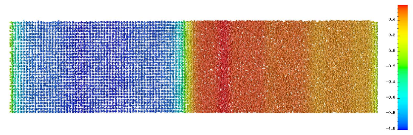
Figure 1. A Lennard-Jones molecular dynamics simulation of a phase transition with periodic boundary conditions, from  [36]. The left part is solid and the right is liquid. The color measures the local potential energy.

The second step to check the accuracy is to derive error estimates. We have three types of error: time discretization error, sampling error and modeling error. The time discretization error comes from approximating the differential equation for molecular dynamics with a numerical method, based on replacing time derivatives with difference quotients for a positive step size $\Delta t$. The sampling error is due to truncating the infinite $T$ and using a finite value of $T$ in the integral in (1.1). The modeling error (also called coarse-graining error) originates from eliminating the electrons in the Schrödinger nuclei-electron system and replacing the nuclei dynamics with their classical paths; this approximation error was first analyzed by Born and Oppenheimer in their seminal paper  [2].

The time discretization and truncation error components are in some sense simple to handle by comparing simulations with different choice of $\Delta t$ and $T$, although it can, of course, be difficult to know that the behavior does not change with even smaller $\Delta t$ and larger $T$. The modeling error is more difficult to check since a direct approach would require to solve the Schrödinger equation. Currently the Schrödinger partial differential equation can only be solved with few particles, therefore it is not an option to solve the Schrödinger equation in general. The reason to use molecular dynamics is precisely in avoiding solution of the Schrödinger equation. Consequently the modeling error requires mathematical error analysis. In the literature there seems to be no error analysis that is precise, simple and constructive enough so that a molecular dynamics simulation can use it to asses the modeling error. Our alternative error analysis presented here is developed with the aim to allow the construction of algorithms that estimate the modeling error in molecular dynamics computations. Our analysis differs from previous ones by using

• the time-independent Schrödinger equation as the reference model to compare molecular dynamics with,

• an amplitude function in a WKB-Ansatz that depends only on position coordinates $(x,X)$ (and not on momentum coordinates $(p,P)$) for caustic states,

• actual solutions of the Schrödinger equation (and not only asymptotic solutions),

• the theory of Hamilton-Jacobi partial differential equations to derive estimates for the corresponding Hamiltonian systems, i.e., the molecular dynamics systems.

Understanding both the exact Schrödinger model and the molecular dynamics model through Hamiltonian systems allows us to obtain bounds for the difference of the solutions by well-established comparison results for the solutions of Hamilton-Jacobi equations, by regarding the Schrödinger Hamiltonian and the molecular dynamics Hamiltonians as perturbations of each others. The Hamilton-Jacobi theory applied to Hamiltonian systems is inspired by the error analysis of symplectic methods for optimal control problems for partial differential equations,  [30]. The result is that the modeling error can be estimated based on the difference of the Hamiltonians, for the molecular dynamics system and the Schrödinger system, along the same solution path, see Theorem 5.1 and Section 6.2.

2. The Schrödinger and molecular dynamics models

In deriving the approximation of the solutions to the full Schrödinger equation the heavy particles are often treated within classical mechanics, i.e., by defining the evolution of their positions and momenta by equations of motions of classical mechanics. Therefore we denote $X_{t}:[0,\infty)\to\mathbb{R}^{3N}$ and $P_{t}:[0,\infty)\to\mathbb{R}^{3N}$ time-dependent functions of positions and momenta with time derivatives denoted by

$${\dot{X_{t}}}=\frac{dX_{t}}{dt}\,,\;\;{\ddot{X_{t}}}=\frac{d^{2}X_{t}}{dt^{2}}\,.$$

We denote the Euclidean scalar product on $\mathbb{R}^{3N}$ by

$${X}\cdot{Y}=\sum_{i=1}^{3N}X^{i}Y^{i}\,.$$

Furthermore, we use the notation $\nabla_{X}\psi(x,X)=(\nabla_{X^{1}}\psi(x,X),\dots,\nabla_{X^{N}}\psi(x,X))$, and as customary $\nabla_{X^{i}}\psi=(\partial_{X_{1}^{i}}\psi,\partial_{X_{2}^{i}}\psi,\partial_{X_{3}^{i}}\psi)$.

On the other hand, the light particles are treated within the quantum mechanical description and the following complex valued bilinear map $\langle{\cdot\,},{\cdot}\rangle:L^{2}(\mathbb{R}^{3n}\times\mathbb{R}^{3N})\times L^{2}(\mathbb{R}^{3n}\times\mathbb{R}^{3N})\to L^{2}(\mathbb{R}^{3N})$ will be used in the subsequent calculations

(2.1) $$\langle{\phi},{\psi}\rangle=\int_{\mathbb{R}^{3n}}\phi(x,X)^{*}\psi(x,X)\,dx\,.$$

The notation $\psi(x,X)=\mathcal{O}(M^{-\alpha})$ is also used for complex valued functions, meaning that $|\psi(x,X)|=\mathcal{O}(M^{-\alpha})$ holds uniformly in $x$ and $X$.

The time-independent Schrödinger equation

(2.2) $$\mathcal{H}(x,X)\Phi(x,X)=E\Phi(x,X)$$

models many-body (nuclei-electron) quantum systems and is obtained from minimization of the energy in the solution space of wave functions, see  [32, 31, 1, 34, 7]. It is an eigenvalue problem for the energy $E\in\mathbb{R}$ of the system in the solution space, described by wave functions, $\Phi:\mathbb{R}^{3n}\times\mathbb{R}^{3N}\to\mathbb{C}$, depending on electron coordinates $x=(x^{1},\ldots,x^{n})\in\mathbb{R}^{3n}$, nuclei coordinates $X=(X^{1},\ldots,X^{N})\in\mathbb{R}^{3N}$, and the Hamiltonian operator $\mathcal{H}(x,X)$

(2.3) $$\mathcal{H}(x,X)=\mathcal{V}(x,X)-\frac{1}{2}M^{-1}\sum_{n=1}^{N}\Delta_{X^{n}}\,.$$

We assume that a quantum state of the system is fully described by the wave function $\Phi:\mathbb{R}^{3n}\times\mathbb{R}^{3N}\to\mathbb{C}$ which is an element of the Hilbert space of wave functions with the standard complex valued scalar product

$$\langle\!\langle\Phi,\Psi\rangle\!\rangle=\int_{\mathbb{R}^{3n}\times\mathbb{R}^{3N}}\Phi(x,X)^{*}\Psi(x,X)\,dx\,dX\,,$$

and the operator $\mathcal{H}$ is self-adjoint in this Hilbert space. The Hilbert space is then a subset of $L^{2}(\mathbb{R}^{3n}\times\mathbb{R}^{3N})$ with symmetry conditions based on the Pauli exclusion principle for electrons, see  [7, 22].

In computational chemistry the operator $\mathcal{V}$, the electron Hamiltonian, is independent of $M$ and it is precisely determined by the sum of the kinetic energy of electrons and the Coulomb interaction between nuclei and electrons. We assume that the electron operator $\mathcal{V}(\cdot,X)$ is self-adjoint in the subspace with the inner product $\langle{\cdot},{\cdot}\rangle$ of functions in (2.1) with fixed $X$ coordinate and acts as a multiplication on functions that depend only on $X$. An essential feature of the partial differential equation (2.2) is the high computational complexity of finding the solution in an antisymmetric/symmetric subset of the Sobolev space $H^{1}(\mathbb{R}^{3n}\times\mathbb{R}^{3N})$. The mass of the nuclei, which are much greater than one (electron mass), are the diagonal elements in the diagonal matrix $M$.

In contrast to the Schrödinger equation, a molecular dynamics model of $N$ nuclei $X:[0,T]\to\mathbb{R}^{3N}$, with a given potential $V_{p}:\mathbb{R}^{3N}\to\mathbb{R}$, can be computationally studied for large $N$ by solving the ordinary differential equations

(2.4) $$\ddot{X}_{t}=-\nabla_{X}V_{p}(X_{t})\,,$$

in the slow time scale, where the nuclei move $\mathcal{O}(1)$ in unit time. This computational and conceptual simplification motivates the study to determine the potential and its implied accuracy compared with the the Schrödinger equation, as started already in the 1920’s with the Born-Oppenheimer approximation [2]. The purpose of our work is to contribute to the current understanding of such derivations by showing convergence rates under new assumptions. The precise aim in this paper is to estimate the error

(2.5) $$\frac{\int_{\mathbb{R}^{3N+3n}}g(X)\Phi(x,X)^{*}\Phi(x,X)\,dx\,dX}{\int_{\mathbb{R}^{3N+3n}}\Phi(x,X)^{*}\Phi(x,X)\,dx\,dX}-\lim_{T\to\infty}\frac{1}{T}\int_{0}^{T}g(X_{t})\,dt$$

for a position dependent observable $g(X)$ of the time-indepedent Schrödinger equation (2.2) approximated by the corresponding molecular dynamics observable $\lim_{T\to\infty}T^{-1}\int_{0}^{T}g(X_{t})\,dt$, which is computationally cheaper to evaluate with several nuclei. The Schrödinger eigenvalue problem may typically have multiple eigenvalues and the aim is to find an eigenfunction $\Phi$ and a molecular dynamics system that can be compared. There may be eigenfunctions that we cannot approximate, but with some assumptions on the spectrum of $\mathcal{V}(\cdot,X)$ the molecular dynamics in fact approximates the observable corresponding to one eigenfunction.

The main step to relate the Schrödinger wave function and the molecular dynamics solution is the so-called zero-order Born-Oppenheimer approximation, where $X_{t}$ solves the classical ab initio molecular dynamics (2.4) with the potential $V_{p}:\mathbb{R}^{3N}\to\mathbb{R}$ determined as an eigenvalue of the electron Hamiltonian $\mathcal{V}(\cdot,X)$ for a given nuclei position $X$. That is $V_{p}(X)=\lambda_{0}(X)$ and

$$\mathcal{V}(\cdot,X)\Psi_{{\mathrm{BO}}}(\cdot,X)=\lambda_{0}(X)\Psi_{{\mathrm{BO}}}(\cdot,X)\,,$$

for an electron eigenfunction $\Psi_{{\mathrm{BO}}}(\cdot,X)\in L^{2}(\mathbb{R}^{3n})$, for instance, the ground state. The Born-Oppenheimer expansion [2] is an approximation of the solution to the time-independent Schrödinger equation which is shown in  [15, 19] to solve the time-independent Schrödinger equation approximately. This expansion, analyzed by the methods of multiple scales, pseudo-differential operators and spectral analysis in  [15, 19, 13], can be used to study the approximation error (2.5). However, in the literature, e.g., [24], it is easier to find precise statements on the error for the setting of the time-dependent Schrödinger equation, since the stability issue is more subtle in the eigenvalue setting.

Instead of an asymptotic expansion we use a different method based on a Hamiltonian dynamics formulation of the time-independent Schrödinger eigenfunction and the stability of the corresponding perturbed Hamilton-Jacobi equations viewed as a hitting problem. This approach makes it possible to reduce the error propagation on the infinite time interval to finite time excursions from a certain co-dimension one hitting set. A motivation for our method is that it forms a sub-step in trying to estimate the approximation error using only information available in molecular dynamics simulations.

The related problem of approximating observables to the time-dependent Schrödinger equation by the Born-Oppenheimer expansions is well studied, theoretically in  [4, 28] and computationally in  [20] using the Egorov theorem. The Egorov theorem shows that finite time observables of the time-dependent Schrödinger equation are approximated with $\mathcal{O}(M^{-1})$ accuracy by the zero-order Born-Oppenheimer dynamics with an electron eigenvalue gap. In the special case of a position observable and no electrons (i.e., $\mathcal{V}=V(X)$ in (2.3)), the Egorov theorem states that

(2.6) $$\left|\int_{\mathbb{R}^{3N}}g(X)\Phi(X,t)^{*}\Phi(X,t)\,dX-\int_{\mathbb{R}^{3N}}g(X_{t})\Phi(X_{0},0)^{*}\Phi(X_{0},0)\,dX_{0}\right|\leq C_{t}M^{-1}\,,$$

where $\Phi(X,t)$ is a solution to the time-dependent Schrödinger equation

$$i\partial_{t}\Phi(\cdot,t)=\mathcal{H}\Phi(\cdot,t)$$

with the Hamiltonian (2.3) and the path $X_{t}$ is the nuclei coordinates for the dynamics with the Hamiltonian $\tfrac{1}{2}|\dot{X}|^{2}+V(X)$. If the initial wave function $\Phi(X,0)$ is the eigenfunction in (2.2) the first term in (2.6) reduces to the first term in (2.5) and the second term can also become the same in an ergodic limit. However, since we do not know that the parameter $C_{t}$ (bounding an integral over $(0,t)$) is bounded for all time we cannot directly conclude an estimate for (2.5) from (2.6).

In our perspective studying the time-independent instead of the time-dependent Schrödinger equation has the important differences that

• the infinite time study of the Born-Oppenheimer dynamics can be reduced to a finite time hitting problem,

• the computational and theoretical problem of specifying initial data for the Schrödinger equation is avoided, and

• computationally cheap evaluation of the position observable $g(X)$ is possible using the time average $\lim_{T\to\infty}\tfrac{1}{T}\int_{0}^{T}g(X_{t})\,dt$ along the solution path $X_{t}$.

In this paper we derive the Born-Oppenheimer approximation from the time-independent Schrödinger equation (2.2) and we establish convergence rates for molecular dynamics approximations to time-independent Schrödinger observables under simple assumptions including the so-called caustic points, where the Jacobian determinant $\det J(X_{t})\equiv\det(\partial X_{t}/\partial X_{0})$ of the Eulerian-Lagrangian transformation of $X$-paths vanish. As mentioned previously, the main new analytical idea is an interpretation of the time-independent Schrödinger equation (2.2) as a Hamiltonian system and the subsequent analysis of the approximations by comparing Hamiltonians. This analysis employs the theory of Hamilton-Jacobi partial differential equations. The problematic infinite-time evolution of perturbations in the dynamics is solved by viewing it as a finite-time hitting problem for the Hamilton-Jacobi equation, with a particular hitting set. In contrast to the traditional rigorous and formal asymptotic expansions we analyze the transport equation as a time-dependent Schrödinger equation.

The main inspiration for this paper are works  [27, 6, 5] and the semi-classical WKB analysis in  [25]: the works  [27, 6, 5] derive the time-dependent Schrödinger dynamics of an $x$-system, $i{\dot{\Psi}}=\mathcal{H}_{1}\Psi,$ from the time-independent Schrödinger equation (with the Hamiltonian $\mathcal{H}_{1}(x)+\epsilon\,\mathcal{H}(x,X)$) by a classical limit for the environment variable $X$, as the coupling parameter $\epsilon$ vanishes and the mass $M$ tends to infinity; in particular  [27, 6, 5] show that the time derivative enters through the coupling of $\Psi$ with the classical velocity. Here we refine the use of characteristics to study classical ab initio molecular dynamics where the coupling does not vanish, and we establish error estimates for Born-Oppenheimer approximations of Schrödinger observables. The small scale, introduced by the perturbation

$$-(2M)^{-1}\sum_{k}\Delta_{X^{k}}$$

of the potential $\mathcal{V}$, is identified in a modified WKB eikonal equation and analyzed through the corresponding transport equation as a time-dependent Schrödinger equation along the eikonal characteristics. This modified WKB formulation reduces to the standard semi-classical approximation, see  [25], in the case of the potential function $\mathcal{V}=V(X)\in\mathbb{R}$, depending only on nuclei coordinates, but becomes different in the case of operator-valued potentials studied here. The global analysis of WKB functions was initiated by Maslov in the 1960’,  [25], and lead to the subject Geometry of Quantization, relating global classical paths to eigenfunctions of the Schrödinger equation, see  [10]. The analysis presented in this paper is based on a Hamiltonian system interpretation of the time-independent Schrödinger equation. Stability of the corresponding Hamilton-Jacobi equation, bypasses the usual separation of nuclei and electron wave functions in the time-dependent self-consistent field equations, [3, 23, 35].

Theorem 5.1 demonstrates that observables from the zero-order Born-Oppenheimer dynamics approximate observables for the Schrödinger eigenvalue problem with the error of order $\mathcal{O}(M^{-1+\delta})$, for any $\delta>0$, assuming that the electron eigenvalues satisfy a spectral gap condition. The result is based on the Hamiltonian (2.3) with any potential $\mathcal{V}$ that is smooth in $X$, e.g., a regularized version of the Coulomb potential. The derivation does not assume that the nuclei are supported on small domains; in contrast derivations based on the time-dependent self-consistent field equations require nuclei to be supported on small domains. The reason that the small support is not needed here comes from the combination of the characteristics and sampling from an equilibrium density. In other words, the nuclei paths behave classically although they may not be supported on small domains. Section 4 shows that caustics couple the WKB modes, as is well-known from geometric optics, see  [18, 25], and generate non-orthogonal WKB modes that are coupled in the Schrödinger density. On the other hand, with a spectral gap and without caustics the Schrödinger density is asymptotically decoupled into a simple sum of individual WKB densities. Section 7 constructs a WKB-Fourier integral Schrödinger solution for caustic states. Section 5.2 relates the approximation results to the accuracy of symplectic numerical methods for molecular dynamics.

A unique property of the time-independent Schrödinger equation we use is the interpretation that the dynamics $X_{t}\in\mathbb{R}^{3N}$ can return to a co-dimension one surface $I$ which then can reduce the dynamics to a hitting time problem with finite-time excursions from $I$. Another advantage of viewing the molecular dynamics as an approximation of the eigenvalue problem is that stochastic perturbations of the electron ground state can be interpreted as a Gibbs distribution of degenerate nuclei-electron eigenstates of the Schrödinger eigenvalue problem (2.2), see  [33]. The time-independent eigenvalue setting also avoids the issue on “wave function collapse” to an eigenstate, present in the time-dependent Schrödinger equation.

We believe that these ideas can be further developed to better understanding of molecular dynamics simulations. For example, it would be desirable to have more precise conditions on the data (i.e. molecular dynamics initial data and potential $\mathcal{V}$) instead of our implicit assumption on finite hitting time and convergence of the Born-Oppenheimer power series approximation in Lemma 6.2.

3. A time-independent Schrödinger WKB-solution

3.1. Exact Schrödinger dynamics

For the sake of simplicity we assume that all nuclei have the same mass. If this is not the case, we can introduce new coordinates $M_{1}^{1/2}\tilde{X}^{k}=M^{1/2}_{k}X^{k}$, which transform the Hamiltonian to the form we want ${\mathcal{V}(x,M_{1}^{1/2}M^{-1/2}\tilde{X})}-(2M_{1})^{-1}\sum_{k=1}^{N}\Delta_{\tilde{X}^{k}}$. The singular perturbation $-(2M)^{-1}\sum_{k}\Delta_{X^{k}}$ of the potential $\mathcal{V}$ introduces an additional small scale $M^{-1/2}$ of high frequency oscillations, as shown by a WKB-expansion, see  [29, 17, 16, 26]. We shall construct solutions to (2.2) in such a WKB-form

(3.1) $$\Phi(x,X)=\phi(x,X)e^{iM^{1/2}\theta(X)}\,,$$

where the amplitude function $\phi:\mathbb{R}^{3n}\times\mathbb{R}^{3N}\to\mathbb{C}$ is complex valued, the phase $\theta:\mathbb{R}^{3N}\to\mathbb{R}$ is real valued, and the factor $M^{1/2}$ is introduced in order to have well-defined limits of $\phi$ and $\theta$ as $M\to\infty$. Note that it is trivially always possible to find funtions $\phi$ and $\theta$ satisfying (3.1), even in the sense of a true equality. Of course, the ansatz only makes sense if $\phi$ and $\theta$ do not have strong oscillations for large $M$. The standard WKB-construction, [25, 16], is based on a series expansion in powers of $M^{1/2}$ which solves the Schrödinger equation with arbitrary high accuracy. Instead of an asymptotic solution, we introduce an actual solution based on a time-dependent Schrödinger transport equation. This transport equation reduces to the formulation in  [25] for the case of a potential function $\mathcal{V}=V(X)\in\mathbb{R}$, depending only on nuclei coordinates $X\in\mathbb{R}^{3N}$, and modifies it for the case of a self-adjoint potential operator $\mathcal{V}(\cdot,X)$ on the electron space $L^{2}(\mathbb{R}^{3n})$ which is the primary focus of our work here. In Sections 4 and 7 we use a linear combination of WKB-eigensolutions, but first we study the simplest case of a single WKB-eigensolution as motivated by the following subsection.

3.1.1. Molecular dynamics from a piecewise constant electron operator on a simplex mesh

The purpose of this section is to convey a first formal understanding of the relation between ab initio molecular dynamics $\ddot{X}_{t}=-\nabla_{X}\lambda_{0}(X_{t})$ and the Schrödinger eigenvalue problem (2.2) and motivate the WKB ansatz (3.1). In subsequent sections we will describe precise analysis of error estimates for the WKB-method. The idea behind this first study is to approximate the electron operator $\mathcal{V}$ by a finite dimensional matrix $\mathcal{V}^{h}$, which is piecewise constant on a simplex mesh in the variable $X$, with the mesh size $h$. Furthermore, we introduce the change of variables

$$\Phi=\sum_{j=0}^{J}\varphi_{j}\Psi_{j}=:\Psi\varphi$$

based on the piecewise constant electron eigenvalues and eigenvectors $\mathcal{V}^{h}\Psi_{j}=\lambda_{j}^{h}\Psi_{j},\ \langle\Psi_{j},\Psi_{j}\rangle=1,\ j=0,\ldots J$, normalized and ordered with respect to increasing eigenvalues. Then the Schrödinger equation (2.2) becomes

$$-\frac{1}{2M}\Delta_{X}(\Psi\varphi)+\mathcal{V}^{h}\Psi\varphi=E\Psi\varphi\,,$$

with the notation $\Delta_{X}=\sum_{j}\Delta_{X_{j}}$, so that on each simplex

$$-\frac{1}{2M}\Delta_{X}\varphi_{j}+\lambda_{j}^{h}\varphi_{j}=E\varphi_{j}\,,$$

which by separation of variables, for each $j=0,1,2,\ldots,J$, implies

(3.2) $$\varphi_{j}=\sum_{P^{j}}a({P^{j}})e^{iM^{1/2}P^{j}\cdot X}$$

for any $P^{j}\in\mathbb{C}^{3N}$ that satisfies the eikonal equation

$$\frac{1}{2}{P^{j}}\cdot{P^{j}}+\lambda_{j}^{h}=E\,,$$

for any $a(P^{j})\in\mathbb{C}$, if all components of $P^{j}$ are non zero. If $P^{j}_{k}=0$ we have $a(P^{j})=\prod_{\{k\,:\,P^{j}_{k}=0\}}(A_{k}X_{k}+B_{k})$ for any $A_{k}\in\mathbb{C},B_{k}\in\mathbb{C}$, since $e^{\pm iM^{1/2}P^{j}_{k}X_{k}}=1$ in this case. The solution $\Phi$, to (2.2), and its normal derivative are continuous at the interfaces of the simplices. On the intersection of the faces the normal derivative is not defined but this set is of measure zero and thus negligible as seen from the $H^{1}(\mathbb{R}^{3N})$ solution concept of (2.2).

We investigate a simpler, one-dimensional case, $X\in\mathbb{R}$, first. Then the solution $\varphi$ simplifies to

$$\varphi_{j}=a_{j}e^{iM^{1/2}P^{j}\cdot X}+b_{j}e^{-iM^{1/2}P^{j}\cdot X}$$

for $a_{j},b_{j},P^{j}\in\mathbb{C}$ and $(P^{j})^{2}/2+\lambda_{j}=E$ . The continuity conditions

(3.3) $$\begin{split}\lim_{X\rightarrow X_{0}+}\Phi(X)&=\lim_{X\rightarrow X_{0}-}\Phi(X)\\ \lim_{X\rightarrow X_{0}+}\partial_{X}\Phi(X)&=\lim_{X\rightarrow X_{0}-}\partial_{X}\Phi(X)\\ \end{split}$$

hold for any $X_{0}\in\mathbb{R}$, in particular, at the interval boundary where for $X_{0}=0$

(3.4) $$\begin{split}\lim_{X\rightarrow X_{0}\pm}\Phi(X)&=\sum_{j}(a_{j\pm}\Psi_{j\pm}+b_{j\pm}\Psi_{j\pm})\\ \lim_{X\rightarrow X_{0}\pm}\partial_{X}\Phi(X)&=iM^{1/2}\sum_{j}(a_{j\pm}P^{j}_{\pm}\Psi_{j\pm}-b_{j\pm}P^{j}_{\pm}\Psi_{j\pm})\,.\\ \end{split}$$

It is clear that given $a_{-}$ and $b_{-}$ we can determine $a_{+}$ and $b_{+}$ so that (3.3) holds. In order to prepare for the multi-dimensional case it is convenient to consider each incoming wave $a_{-}$ and $b_{+}$ separately: the incoming $a_{-}$ wave is split into a refracted $a_{+}$ and reflected $b_{-}$ wave

(3.5) $$\sum_{j}a_{j-}\Psi_{j-}P^{j}_{-}=\sum_{j}(a_{j+}\Psi_{j+}P^{j}_{+}+b_{j-}\Psi_{j-}P^{j}_{-})$$

and similarly the incoming $b_{+}$ wave is split into a refracted $b_{-}$ wave and a reflected $a_{+}$ wave, see Figure 2. The jump conditions at the different interfaces are coupled by the oscillatory functions $e^{\pm iM^{1/2}P^{j}\cdot X}$. The global construction of $\varphi$ and $\Psi$ in one dimension follows by marching in the positive $X$-direction to successive intervals, creating in each interval both a $e^{iM^{1/2}P^{j}\cdot X}\Psi_{j}$ and a $e^{-iM^{1/2}P^{j}\cdot X}\Psi_{j}$ wave.

In general each interface condition (3.4) also couples all eigenvectors $\Psi_{j}$. However, we shall see that if $M$ is large, $\mathcal{V}$ smooth and there is a spectral gap $\lambda_{1}-\lambda_{0}>c>0$ then, in the limit of the simplex size $h$ tending to zero, there is an asymptotically uncoupled WKB-solution $\Phi(x,X)=\phi(x,X)e^{iM^{1/2}\theta(X)}$, where $\theta:\mathbb{R}^{3N}\rightarrow\mathbb{R},\ \phi:\mathbb{R}^{3n}\times\mathbb{R}^{3N}\rightarrow\mathbb{C}$. Under these assumptions the Born-Oppenheimer approximation in Lemma 6.2 shows that $\phi$ is asymptotically parallel, in $L^{2}(dx)$, to the electron eigenfunction $\Psi_{0}$ as $M\rightarrow\infty$. The gradient $\nabla_{X}\theta(X)=P^{0}$ is obtained from the differential $\theta(X)=\theta(X_{0})+\nabla_{X}\theta(X_{0})\cdot(X-X_{0})+o(|X-X_{0}|)$.

In the case of electron eigenvalue crossing, i.e., $\lambda_{1}(X)=\lambda_{0}(X)$ for some $X$, or so called avoided crossings (meaning that the eigenvalue gap $c\ll 1$ is small and dependent on $M$), a refraction will, in general, include all components $a_{j}e^{iM^{1/2}{P^{j}}\cdot{X}}\Psi_{j},\ j=1,\ldots,J$ and consequently the Born-Oppenheimer approximation fails.

The construction of a solution to the Schrödinger equation with a piecewise constant potential is more involved in the multi-dimensional case for two reasons: each reflection at an interface generates, in general, an additional path in a new direction, so that many paths are needed. Furthermore, the construction of a solution to the eikonal equation is more complicated since the jump condition (3.4) implies that the tangential component $P^{j}_{t}$ of $P^{j}$ must be continuous across a simplex face and only the normal component $P^{j}_{n}=P^{j}-P^{j}_{t}$ may have a jump. In multi-dimensional cases it is still possible to construct a solution of the form (3.2) by following the characteristic paths $\dot{X}_{t}=P^{j}(X_{t})$ and using the jump conditions (3.4): when the path $X_{t}$ hits a simplex face, the tangential part $P^{j}_{t}$ of $P^{j}$ is continuous and the normal component $P^{j}_{n}$ of $P^{j}$ may jump. At a simplex face the new value of the $P^{j}_{n}$ is determined by $({P^{j}_{n}}\cdot{P^{j}_{n}}+{P^{j}_{t}}\cdot{P^{j}_{t}})/2+\lambda_{j}^{h}=E$. Analogously to the one dimensional case we treat the pair $e^{iM^{1/2}{(P^{j}_{t}+P^{j}_{n})}\cdot{X}}$ and $e^{iM^{1/2}{(P^{j}_{t}-P^{j}_{n})}\cdot{X}}$ together. However, each collision with $e^{iM^{1/2}{(P^{j}_{t}+P^{j}_{n})}\cdot{X}}$ on an interface now creates a reflected wave in another direction, in particular, $e^{iM^{1/2}{(P^{j}_{t}-P^{j}_{n})}\cdot{X}}\Psi_{j}$, and we get many paths to follow. Therefore each mode $e^{iM^{1/2}{P^{j}}\cdot{X}}$ follows its characteristic $X_{t}$, where $\dot{X}_{t}=P^{j}$, through the simplex to the adjacent simplicial faces, which the characteristic pass through when they leave the simplex, and at these outflow faces a reflected mode is created and a refracted mode continues into the adjacent simplices, see Figure 2. In this way we can formally construct a solution of the form $\sum_{P^{j}}a({P^{j}})e^{iM^{1/2}P^{j}\cdot X}\Psi_{j}$ to the Schrödinger equation (2.2), with possibly several different characteristic paths in each simplex.

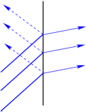
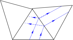
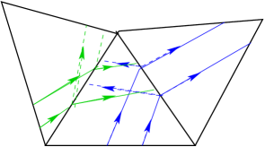
Figure 2. The value of $P^{j}$ is constructed by following the characteristic paths $X_{t}$ (the blue and green curves), based on $\dot{X}_{t}=P^{j}$, with a reflection-refraction at each simplex face (left) following the path through simplices (middle) and each simplex may have several $P^{j}$ (right).

In conclusion, the piecewise constant electron operator shows that the solution to the Schrödinger equation (2.2) is composed of a linear combination of highly oscillatory function modes $a_{j}e^{iM^{1/2}P^{j}\cdot X}\Psi_{j}$ based on the electron eigenvectors $\Psi_{j}$ and eigenvalues $\lambda_{j}$, where $P^{j}$ satisfies the eikonal equation $P^{j}\cdot P^{j}/2+\lambda_{j}(X)=E$. These modes can be followed be characteristics $\dot{X}=P^{j}$ from simplex to simplex. In this paper we show that observables based on the related WKB Schrödinger solutions can be approximated by molecular dynamics time averages, when there is a spectral gap around $\lambda_{0}$.

3.1.2. A first WKB-solution

The WKB-solution satisfies the Schrödinger equation (2.2) provided that

(3.6) $$\begin{split}0&=(\mathcal{H}-E)\phi\,\,e^{iM^{1/2}\theta(X)}\\ &=\left((\frac{1}{2}|\nabla_{X}\theta|^{2}+\mathcal{V}-E)\phi\right.-\frac{1}{2M}\Delta_{X}\phi-\frac{i}{M^{1/2}}({\nabla_{X}\phi}\cdot{\nabla_{X}\theta}\left.+\frac{1}{2}\phi\,\Delta_{X}\theta)\right)\,e^{iM^{1/2}\theta(X)}\,.\end{split}$$

We shall see that only eigensolutions $\Phi$ that correspond to dynamics without caustics correspond to such a single WKB-mode, as for instance when the eigenvalue $E$ is inside an electron eigenvalue gap. Solutions in the presence of caustics use a Fourier integral of such WKB-modes, and we treat this case in detail in Section 7. To understand the behavior of $\theta$, we multiply (3.6) by $\phi^{*}e^{-iM^{1/2}\theta(X)}$ and integrate over $\mathbb{R}^{3n}$. Similarly we take the complex conjugate of (3.6), and multiply by $\phi\,e^{iM^{1/2}\theta(X)}$ and integrate over $\mathbb{R}^{3n}$. By adding these two expressions we obtain

(3.7) $$\begin{split}0&=2\big{(}\frac{1}{2}|\nabla_{X}\theta|^{2}-E\big{)}\,\langle{\phi},{\phi}\rangle+\underbrace{\langle{\phi},{\mathcal{V}\phi}\rangle+\langle{\mathcal{V}\phi},{\phi}\rangle}_{=2\langle{\phi},{\mathcal{V}\phi}\rangle}-\frac{1}{2M}\left(\langle{\phi},{\Delta_{X}\phi}\rangle+\langle{\Delta_{X}\phi},{\phi}\rangle\right)\\ &{}-\frac{i}{M^{1/2}}\underbrace{\big{(}\langle{\phi},{{\nabla_{X}\phi}\cdot{\nabla_{X}\theta}}\rangle-\langle{{\nabla_{X}\phi}\cdot{\nabla_{X}\theta}},{\phi}\rangle\big{)}}_{=2i\mathrm{Im}\,\langle{\phi},{{\nabla_{X}\phi}\cdot{\nabla_{X}\theta}}\rangle}+\frac{i}{2M^{1/2}}\underbrace{\big{(}\langle{\phi},{\phi}\rangle-\langle{\phi},{\phi}\rangle\big{)}}_{=0}\Delta_{X}\theta\,.\end{split}$$

The purpose of the phase function $\theta$ is to generate an accurate approximation in the limit as $M\to\infty$. A possible and natural definition of $\theta$ would be the formal limit of (3.7) as $M\to\infty$, which is the Hamilton-Jacobi equation, also called the eikonal equation

(3.8) $$\frac{1}{2}|\nabla_{X}\theta|^{2}=E-V_{0}\,,$$

where the function $V_{0}:\mathbb{R}^{3N}\to\mathbb{R}$ is

(3.9) $$V_{0}:=\frac{\langle{\phi},{\mathcal{V}\phi}\rangle}{\langle{\phi},{\phi}\rangle}\,.$$

The solution to the Hamilton-Jacobi eikonal equation can be constructed from the associated Hamiltonian system

(3.10) $$\begin{split}{\dot{X}}_{t}&=P_{t}\\ {\dot{P}}_{t}&=-\nabla_{X}V_{0}(X_{t})\end{split}$$

through the characteristics path $(X_{t},P_{t})$ satisfying $\nabla_{X}\theta(X_{t})=:P_{t}$. The amplitude function $\phi$ can be determined by requiring the ansatz (3.6) to be a solution, which gives

$$0 = (\mathcal{H}-E)\phi\,e^{iM^{1/2}\theta(X)}$$

$$= \Big{(}\underbrace{(\frac{1}{2}|\nabla_{X}\theta|^{2}+V_{0}-E)}_{=0}\phi$$

$${-\frac{1}{2M}\Delta_{X}\phi+(\mathcal{V}-V_{0})\phi-\frac{i}{M^{1/2}}({\nabla_{X}\phi}\cdot{\nabla_{X}\theta}+\frac{1}{2}\phi\Delta_{X}\theta)\Big{)}}\,e^{iM^{1/2}\theta(X)}\,,$$

so that by using (3.8) we have

$$-\frac{1}{2M}\Delta_{X}\phi+(\mathcal{V}-V_{0})\phi-\frac{i}{M^{1/2}}({\nabla_{X}\phi}\cdot{\nabla_{X}\theta}+\frac{1}{2}\phi\Delta_{X}\theta)=0\,.$$

The usual method for determining $\phi$ from this so-called transport equation uses an asymptotic expansion $\phi\simeq\sum_{k=0}^{K}M^{-k/2}\phi_{k}$, see  [15, 19] and the beginning of Section 6. An alternative is to write it as a Schrödinger equation, similar to work in  [25]: we apply the characteristics in (3.10) to write

$$\frac{d}{dt}\phi(X_{t})={\nabla_{X}\phi}\cdot{{\dot{X}}_{t}}={\nabla_{X}\phi}\cdot{\nabla_{X}\theta}\,,$$

and define the weight function $G$ by

(3.11) $$\frac{d}{dt}\log G_{t}=\frac{1}{2}\Delta_{X}\theta(X_{t})\,,$$

and the variable $\psi_{t}:=\phi(X_{t})G_{t}$. We use the notation $\phi(X)$ instead of the more precise $\phi(\cdot,X)$, so that e.g. $\psi_{t}=\psi_{t}(x)=\phi(x,X_{t})G_{t}$. Then the transport equation becomes a Schrödinger equation

(3.12) $$iM^{-1/2}{\dot{\psi}}_{t}=(\mathcal{V}-V_{0})\psi_{t}-\frac{G_{t}}{2M}\Delta_{X}\left(\frac{\psi_{t}}{G_{t}}\right)\,.$$

In conclusion, equations (3.8)-(3.12) determine the WKB-ansatz (3.1) to be a solution to the Schrödinger equation (2.2).

Theorem 3.1.

Assume the Hamilton-Jacobi equation, with the corresponding Hamiltonian,

$$H_{{\mathrm{S}}}(X,P):=\frac{1}{2}|P|^{2}+\underbrace{\frac{\langle{\psi(X)},{\mathcal{V}(X)\psi(X)}\rangle}{\langle{\psi(X)},{\psi(X)}\rangle}}_{=:V_{0}(X)}-E=0\,,$$

based on the primal variable $X$ and the dual variable $P=P(X)=\nabla_{X}\theta(X)$, has a smooth solution $\theta(X)$, then $\theta$ generates a solution to the time-independent Schrödinger equation $(\mathcal{H}-E)\Phi=0$, in the sense that

$$\Phi(X_{t},x)=\hat{G}^{-1}(X_{t})\hat{\psi}(x,X_{t})e^{iM^{1/2}\theta(X_{t})}\,,$$

solves the equation (2.2), where $\hat{\psi}(X_{t}):=\psi_{t}$ satisfies the transport equation (3.12) and

$$\begin{split}&\hat{G}(X_{t})=G_{t}\,,\\ &\frac{d}{dt}\log G_{t}=\frac{1}{2}\Delta_{X}\theta(X_{t})\,,\\ &\mbox{$(X_{t},P_{t})$ solves the Hamiltonian system \eqref{hj_first} corresponding to $H_{{\mathrm{S}}}$.}\end{split}$$

It is well know that Hamilton-Jacobi equations in general do not have smooth solutions, due to $X$-paths that collide, as seen by (7.25) generating blow up in $\partial_{XX}\theta(X)$. However if the domain is small enough, the data on the boundary is smooth and $V_{0}$ is smooth, then the characteristics generate a smooth solution, see Ref. [12]. In Section 7.2.5 we describe Maslov’s method to find a global solution by patching together local solutions.

Note that the nuclei density, using $\hat{G}$, can be written

(3.13) $$\rho:=\frac{\langle{\phi},{\phi}\rangle}{\int_{\mathbb{R}^{3N}}\langle{\phi},{\phi}\rangle\,dX}=\frac{\langle{\hat{\psi}},{\hat{\psi}}\rangle\,\hat{G}^{-2}}{\int_{\mathbb{R}^{3N}}\langle{\hat{\psi}},{\hat{\psi}}\rangle\,\hat{G}^{-2}\,dX}\,,$$

and since each time $t$ determines a unique point $(X_{t},P_{t})=(X_{t},\nabla_{X}\theta(X_{t}))$ in the phase space the functions $\hat{G}$ and $\hat{\psi}$ are well defined.

3.1.3. Liouville’s Formula

In this section we verify Liouville’s formula

(3.14) $$\frac{G^{2}_{0}}{G_{t}^{2}}=e^{-\int_{0}^{t}\mathrm{Tr}\,\left(\nabla_{X}P(X_{t})\right)\,dt}=\left|\det\frac{\partial(X_{0})}{\partial(X_{t})}\right|\,,$$

given in  [25]. The characteristic ${\dot{X}}_{t}=P(X_{t})$ implies $\tfrac{d}{dt}{J({X_{t}})}=\nabla_{X}P\,{J({X})}$, where ${J({X})}_{ij}=\partial X^{i}_{t}/\partial X^{j}_{0}$ denotes the first variation with respect to perturbations of the initial data. The logarithmic derivative then satisfies $d/dt\big{(}\log{J({X})}\big{)}_{ij}=\partial_{X^{j}}P^{i}(X_{t})=\partial_{X^{i}X^{j}}\theta(X)$ which implies that $\log{J({X_{t}})}$ is symmetric and shows that (3.14) holds

$${\mathrm{div}}P=\mathrm{Tr}\,\nabla_{X}P=\frac{d}{dt}\mathrm{Tr}\,\log{J({X})}=\frac{d}{dt}\log\det{J({X})}\,.$$

The last step uses that ${J({X})}$ can be diagonalized by an orthogonal transformation and that the trace is invariant under orthogonal transformations.

3.1.4. Data for the Hamiltonian system

For the energy $E$ chosen larger than the potential energy, that is such that $E\geq V_{0}$, the Hamiltonian system (3.10) yields a solution $(X,P):[0,T]\rightarrow U\times\mathbb{R}^{3N}$ to the eikonal equation (3.8) locally in a neighborhood $U\subseteq\mathbb{R}^{3N}$, for regular compatible data $(X_{0},P_{0})$ given on a $3N-1$ dimensional ”inflow”-domain $I\subset\overline{U}$. Typically, the domain $I$ and the data $(X_{0},P_{0})|_{I}$ are not given (except that its total energy is $E$), unless it is really an inflow domain and characteristic paths do not return to $I$ as in a scattering problem. If paths leaving from $I$ return to $I$, there is an additional compatibility of data on $I$: assume $X_{0}\in I$ and $X_{t}\in I$, then the values $P_{t}$ are determined from $P_{0}$; continuing the path to subsequent hitting points $X_{t_{j}}\in I$, $j=1,2,\ldots$ determines $P_{t_{j}}$ from $P_{0}$. The characteristic path $(X_{t},P_{t})$, $t>0$, generates a manifold in the phase space $(X,P)$, which is smooth under our assumptions. This manifold is in general only locally of the form $(X,P(X))$, but in the case of no caustics it is globally of this form and then there is a phase function $X\mapsto\theta(X)$ such that $P(X)=\nabla_{X}\theta(X)$ globally. In Section 7 we study phase space manifolds with caustics.

Remark 3.2.

The integrating factor $G$ and its derivative $\partial_{X^{i}}G$ can be determined from $(P,\partial_{X^{i}}P,\partial_{X^{i}X^{j}}P)$ along the characteristics by the following characteristic equations obtained from (3.8) by differentiation with respect to $X$

(3.15) $$\begin{split}\frac{d}{dt}{\partial_{X^{r}}P^{k}}&=\left[\sum_{j}P^{j}\partial_{X^{j}X^{r}}P^{k}=\sum_{j}P^{j}\partial_{X^{r}X^{k}}P^{j}\right]\\ &=-\sum_{j}\partial_{X^{r}}P^{j}\partial_{X^{k}}P^{j}-\partial_{X^{r}X^{k}}V_{0}\,,\\ \frac{d}{dt}{\partial_{X^{r}X^{q}}P^{k}}&=\left[\sum_{j}P^{j}\partial_{X^{j}X^{r}X^{q}}P^{k}+\sum_{j}P^{j}\partial_{X^{r}X^{k}X^{q}}P^{j}\right]\\ &=-\sum_{j}\partial_{X^{r}}P^{j}\partial_{X^{k}X^{q}}P^{j}-\sum_{j}\partial_{X^{r}X^{q}}P^{j}\partial_{X^{k}}P^{j}-\partial_{X^{r}X^{k}X^{q}}V_{0}\,,\\ \end{split}$$

and similarly $\partial_{X^{i}X^{j}}G$ can be determined from $(P,\partial_{X^{i}}P,\partial_{X^{i}X^{j}}P,\partial_{X^{i}X^{j}X^{k}}P)$.

3.2. Born-Oppenheimer dynamics

The Born-Oppenheimer approximation leads to the standard formulation of ab initio molecular dynamics, in the micro-canonical ensemble with the constant number of particles, volume and energy, for the nuclei positions $X=X_{{\mathrm{BO}}}$,

(3.16) $$\begin{split}\dot{X}_{t}&=P_{t}\,,\\ \dot{P}_{t}&=-\nabla_{X}\lambda_{0}(X_{t})\,,\end{split}$$

by using that the electrons are in the eigenstate $\psi=\Psi_{{\mathrm{BO}}}$ with eigenvalue $\lambda_{0}$ to $\mathcal{V}$, in $L^{2}(dx)$ for fixed $X$, i.e., $\mathcal{V}(X)\Psi_{{\mathrm{BO}}}=\lambda_{0}(X)\Psi_{{\mathrm{BO}}}$. The corresponding Hamiltonian is $H_{{\mathrm{BO}}}(X,P):=|P|^{2}/2+\lambda_{0}(X)$ with the eikonal equation

(3.17) $$\frac{1}{2}|\nabla_{X}\theta_{{\mathrm{BO}}}(X)|^{2}+\lambda_{0}(X)=E\,.$$

3.3. Equations for the density

We note that

$$\phi=\hat{G}^{-1}\hat{\psi}=\left(\frac{\rho}{\langle{\hat{\psi}},{\hat{\psi}}\rangle/\int\langle{\hat{\psi}},{\hat{\psi}}\rangle\hat{G}^{-2}\,dX}\right)^{1/2}\,\hat{\psi}\,,$$

shows that $G$ and $\psi$ determine the density

(3.18) $$\rho_{{\mathrm{S}}}=\rho=\frac{\langle{\hat{\psi}},{\hat{\psi}}\rangle|\hat{G}|^{-2}}{\int\langle{\hat{\psi}},{\hat{\psi}}\rangle\,|\hat{G}|^{-2}dX}\,,$$

defined in (3.13). Using the Born-Oppenheimer approximation in Lemma 6.2 we have $\langle{\hat{\psi}},{\hat{\psi}}\rangle=1+\mathcal{O}(M^{-1})$ in the case of a spectral gap. Therefore the weight function $|\hat{G}|^{-2}$ approximates the density and we know from Theorem 3.1 that $|\hat{G}|^{-2}$ is determined by the phase function $\theta$.

The Born-Oppenheimer dynamics generates an approximate solution $\Psi_{{\mathrm{BO}}}\hat{G}_{{\mathrm{BO}}}^{-1}e^{iM^{1/2}\theta_{{\mathrm{BO}}}}$ which yields the density

(3.19) $$\rho_{{\mathrm{BO}}}=|\hat{G}_{{\mathrm{BO}}}|^{-2},$$

where

$$\frac{d}{dt}\log|\hat{G}_{{\mathrm{BO}}}|^{-2}=-\Delta_{X}\theta_{{\mathrm{BO}}}(X)\,.$$

This representation can also be obtained from the conservation of mass

(3.20) $$0={\mathrm{div}}(\rho_{{\mathrm{BO}}}\nabla_{X}\theta_{{\mathrm{BO}}})$$

implying

(3.21) $$\frac{d}{dt}{\rho}_{{\mathrm{BO}}}(X_{t})={\nabla_{X}\rho_{{\mathrm{BO}}}(X_{t})}\cdot{\dot{X}_{t}}=-\rho_{{\mathrm{BO}}}(X_{t})\ {\mathrm{div}}\nabla_{X}\theta_{{\mathrm{BO}}}\,,\\$$

with the solution

(3.22) $$\rho_{{\mathrm{BO}}}(X_{t})=\frac{C}{|\hat{G}_{{\mathrm{BO}}}(X_{t})|^{2}}\,,$$

where $C$ is a positive constant for each characteristic. Note that the derivation of this classical density does not need a corresponding WKB equation but uses only the conservation of mass that holds for classical paths satisfying a Hamiltonian system. The classical density corresponds precisely to the Eulerian-Lagrangian change of coordinates $|G_{t}|^{2}/|G_{0}|^{2}=\det(\partial X_{t}/\partial X_{0})$ in (3.14).

3.4. Construction of the solution operator

The WKB Ansatz (3.1) is meaningful when $\psi$ does not include the full small scale. In Lemma 6.2 we present conditions for $\psi$ to be smooth.

To construct the solution operator it is convenient to include a non interacting particle in the system, i.e., a particle without charge, and assume that this particle moves with a constant, high speed $dX_{1}^{1}/dt=P_{1}^{1}\gg 1$ (or equivalently with the unit speed and a large mass). Such a non interacting particle does not affect the other particles. The additional new coordinate $X^{1}_{1}$ is helpful in order to simply relate the time-coordinate $t$ and $X^{1}_{1}$. We add the corresponding kinetic energy $(P^{1}_{1})^{2}/2$ to $E$ in order not to change the original problem (2.2) and write the equation (3.12) in the fast time scale $\tau=M^{1/2}t$

$$i\frac{d}{d\tau}\psi=(\mathcal{V}-V_{0})\psi-\frac{1}{2M}G\sum_{j}\Delta_{X^{j}}(G^{-1}\psi)\,.$$

Furthermore, we change to the coordinates

$$(\tau,X_{*}):=(\tau,X^{1}_{2},X^{1}_{3},X^{2},\ldots,X^{N})\in[0,\infty)\times I\,,\;\;\mbox{instead of $(X^{1},X^{2},\ldots,X^{N})\in\mathbb{R}^{3N}$,}$$

where $X^{j}=(X^{j}_{1},X^{j}_{2},X^{j}_{3})\in\mathbb{R}^{3}$. Hence we obtain

(3.23) $$i\dot{\psi}+\frac{1}{2(P_{1}^{1})^{2}}\ddot{\psi}=(\mathcal{V}-V_{0})\psi-\frac{1}{2M}G\sum_{j}\Delta_{X_{*}^{j}}(G^{-1}\psi)=:\tilde{\mathcal{V}}\psi\,,$$

using the notation $\dot{w}=dw/d\tau$ in this section. In Section 6.1 we show that the left hand side can be reduced to $i\dot{\psi}$ as $P_{1}^{1}\rightarrow\infty$, by choosing special initial data. Note also that $G$ is independent of the first component in $X^{1}$. We see that the operator

$$\bar{\mathcal{V}}:=G^{-1}\tilde{\mathcal{V}}G=\underbrace{G^{-1}(\mathcal{V}-V_{0})G}_{=\mathcal{V}-V_{0}}-\frac{1}{2M}\sum_{j}\Delta_{X^{j}_{*}}$$

is symmetric on $L^{2}(\mathbb{R}^{3n+3N-1})$. Assume now the data $(X_{0},P_{0},Z_{0})$ for $X_{0}\in\mathbb{R}^{3N-1}$ is $(L\mathbb{Z})^{3N-1}$-periodic, then also $(X_{\tau},P_{\tau},Z_{\tau})$ is $(L\mathbb{Z})^{3N-1}$-periodic, for $Z_{t}=\theta(X_{t})$ and $P_{t}=\nabla_{X}\theta(X_{t})$. To simplify the notation for such periodic functions, define the periodic circle

$$\mathbb{T}:=\mathbb{R}/(L\mathbb{Z})\,.$$

We seek a solution $\Phi$ of (2.2) which is $(L\mathbb{Z})^{3(n+N)-1}$-periodic in the $(x,X_{*})$-variable. The Schrödinger operator $\bar{\mathcal{V}}(\cdot,X_{\tau})$ has, for each $\tau$, real eigenvalues $\{\lambda_{m}(\tau)\}$ with a complete set of eigenvectors $\{\zeta^{m}(x,X_{*},\tau)\}$ orthogonal in the space of $x$-anti-symmetric functions in $L^{2}(\mathbb{T}^{3n+3N-1})$, see  [1]. The proof uses that the operator $\bar{\mathcal{V}}_{\tau}+\gamma I$ generates a compact solution operator in the Hilbert space of $x$-anti-symmetric functions in $L^{2}(\mathbb{T}^{3n+3N-1})$, for the constant $\gamma\in(0,\infty)$ chosen sufficiently large. The discrete spectrum and the compactness comes from Fredholm theory for compact operators and the fact that the bilinear form $\int_{\mathbb{T}^{3(n+N)-1}}v\bar{\mathcal{V}}_{\tau}w+\gamma vw\,dx\,dX_{*}$ is continuous and coercive on $H^{1}(\mathbb{T}^{3(n+N)-1})$, see  [12]. We see that $\tilde{\mathcal{V}}$ has the same eigenvalues $\{\lambda_{m}(\tau)\}$ and the eigenvectors $\{G_{\tau}\zeta^{m}(\tau)\}$, orthogonal in the weighted $L^{2}$-scalar product

$$\int_{\mathbb{T}^{3N-1}}\langle{v},{w}\rangle\ \hat{G}^{-2}\,dX_{*}\,.$$

The construction and analysis of the solution operator continues in Section  6.1 based on the spectrum.

Remark 3.3 (Boundary conditions).

The eigenvalue problem (2.2) makes sense not only in the periodic setting but also with alternative boundary conditions from interaction with an external environment, e.g., for scattering problems.

4. Computation of observables

Suppose the goal is to compute a real-valued observable

$$\int_{\mathbb{T}^{3N}}\langle{\Phi},{A\Phi}\rangle\,dX$$

for a given bounded linear multiplication operator $A=A(X)$ on $L^{2}(\mathbb{T}^{3N})$ and a solution $\Phi=\sum_{k}\phi_{k}e^{iM^{1/2}\theta_{k}}$ of (2.2). We have

(4.1) $$\begin{array}[]{ll}\int_{\mathbb{T}^{3N}}\langle{\Phi},{A\Phi}\rangle dX&=\sum_{k,l}\int_{\mathbb{T}^{3N}}\langle{A\phi_{k}e^{iM^{1/2}\theta_{k}(X)}},{\phi_{l}e^{iM^{1/2}\theta_{l}(X)}}\rangle\,dX\\ &=\sum_{k,l}\int_{\mathbb{T}^{3N}}Ae^{iM^{1/2}\left(\theta_{l}(X)-\theta_{k}(X)\right)}\langle{\phi_{k}},{\phi_{l}}\rangle\,dX\,.\end{array}$$

The integrand is oscillatory for $k\neq l$, hence critical points (or near critical points) of the phase difference give the main contribution. The stationary phase method, see  [10, 25] and Section 9, shows that these integrals are small, bounded by $\mathcal{O}(M^{-3N/4})$, in the case when the phase difference has non degenerate critical points, or no critical point, and the functions $A\langle{\phi_{k}},{\phi_{l}}\rangle$ and $\theta_{l}$ are sufficiently smooth. A critical point $X_{c}\in\mathbb{R}^{3N}$ satisfies $\nabla_{X}\theta_{l}(X_{c})-\nabla_{X}\theta_{k}(X_{c})=0$, which means that the two different paths, generated by $\theta_{l}$ and $\theta_{k}$, passing through $X=X_{c}$ also have the same momentum $P$ at this point. That the critical point is degenerate means that the Hessian matrix $\partial_{X^{i}X^{j}}(\theta_{k}-\theta_{l})(X_{c})$ is singular (or asymptotically singular for $M\rightarrow\infty$ as for avoided crossings when the electron eigenvalues have a vanishing spectral gap depending on $M$). Therefore caustics, crossing or avoided crossing electron eigenvalues may generate coupling between the WKB terms. On the other hand, without such coupling the density of a linear combination of WKB terms separates asymptotically to a sum of densities of the individual WKB terms

(4.2) $$\int_{\mathbb{T}^{3N}}\langle{\Phi},{A\Phi}\rangle dX=\sum_{k=1}^{\bar{k}}\int_{\mathbb{T}^{3N}}A\underbrace{\langle{\phi_{k}},{\phi_{k}}\rangle}_{=\rho_{k}}\,dX+\mathcal{O}(M^{-1})\,,$$

in the case of multiple eigenstates, $\bar{k}>1$, and

$$\int_{\mathbb{T}^{3N}}\langle{\Phi},{A\Phi}\rangle\,dX=\int_{\mathbb{T}^{3N}}A\langle{\phi_{1}},{\phi_{1}}\rangle\,dX$$

for a single eigenstate. In the next section we will study molecular dynamics approximations of a single state

(4.3) $$\int_{\mathbb{T}^{3N}}A\langle{\phi_{k}},{\phi_{k}}\rangle\,dX=\int_{\mathbb{T}^{3N}}A(X)\rho_{k}(X)\,dX\,.$$

In the presence of a caustic, the WKB terms can be asymptotically non orthogonal, since their coefficients and phases typically are not smooth enough to allow the integration by parts to gain powers of $M^{-1/2}$. Non-orthogonal WKB functions tell how the caustic couples the WKB modes.

Regarding the inflow density $\rho_{k}\big{|}_{I}$ there are two situations: either the characteristics return often to the inflow domain or not. If they do not return we have a scattering problem and it is reasonable to define the inflow-density $\rho_{k}\big{|}_{I}$ as an initial condition. If characteristics return, the dynamics can be used to estimate the return-density $\rho_{k}\big{|}_{I}$ as follows: Assume that the following limits exist

(4.4) $$\lim_{T\rightarrow\infty}\frac{1}{T}\int_{0}^{T}A(X_{t})\,dt=\int_{\mathbb{T}^{3N}}A(X)\rho_{k}(X)\,dX$$

which bypasses the need to find $\rho_{k}\big{|}_{I}$ and the quadrature in the number of characteristics. A way to think about this limit is to sample the return points $X_{t}\in I$ and from these samples construct an empirical return-density, converging to $\rho_{k}\big{|}_{I}$ as the number of return iterations tends to infinity. We shall use this perspective to view the eikonal equation (3.8) as a hitting problem on $I$, with hitting times $\tau$ (i.e., return times). The property having $\rho|_{I}$ constant as a function of $X_{0}$ is called ergodicity, which we will use. We could allow the density $\rho|_{I}$ to depend on the initial position $X_{0}$ and momentum $P_{0}$, but then our observables need to conditional expected values. An example of a hitting surface is the co-dimension one surface where the first component $X_{11}$ in $X_{1}=(X_{11},X_{12},X_{13})$ is equal to its initial value $X_{11}(0)$. The dynamics does not always have such a hitting surface: for instance if all particles are close initially and then are scattered away from each other, as in an explosion, no co-dimension one hitting surface exists.

5. Molecular dynamics approximation of Schrödinger observables

A numerical computation of an approximation to $\sum_{k}\int_{\mathbb{T}^{3N}}\langle{\phi_{k}},{A\phi_{k}}\rangle\,dX$ has the main ingredients:

• to approximate the exact characteristics by molecular dynamics characteristics (3.10),

• to discretize the molecular dynamics equations, and

• if $\rho\big{|}_{I}$ is an inflow-density, to introduce quadrature in the number of characteristics, or

• if $\rho\big{|}_{I}$ is a return-density, to replace the ensemble average by a time average using the property (4.4).

This section presents a derivation of the approximation error in the step (1) in the case of a return density and comments on the time-discretization of step (2) treated in Section 5.2. The third and fourth discretization steps, which are not described here, are studied, for instance, in  [8, 7, 21].

5.1. The Born-Oppenheimer approximation error

This section states our main result of molecular dynamics approximating Schrödinger observables. We formulate it using the assumption of the Born-Oppenheimer property

(5.1) $$\|\psi_{t}-\Psi_{{\mathrm{BO}}}(X_{t})\|_{L^{2}(dx)}=\mathcal{O}(M^{-1/2})\,,\quad\mbox{uniformly in $t$.}$$

This assumption is then proved in Lemma 6.2 based on a setting with a spectral gap.

The spectral gap condition. The electron eigenvalues $\{\lambda_{k}\}$ satisfy, for some positive $c$, the spectral gap condition

(5.2) $$\inf_{k\neq 0,\ Y\in D}|\lambda_{k}(Y)-\lambda_{0}(Y)|>c\,,$$

where $D:=\{X_{{\mathrm{S}}}(t){\,|\,}t\geq 0\}\cup\{X_{{\mathrm{BO}}}(t){\,|\,}t\geq 0\}$ is the set of all nuclei positions obtained from the Schrödinger characteristics $X=X_{{\mathrm{S}}}$ in Theorem 3.1 and from the Born-Oppenheimer dynamics $X=X_{{\mathrm{BO}}}$ in (3.16), for all considered initial data.

Theorem 5.1.

Assume that the phase functions $\theta_{{\mathrm{S}}}$ and $\theta_{{\mathrm{BO}}}$ are smooth solutions to the eikonal equations (3.8) and (3.17) and that the Born-Oppenheimer property (5.1) holds, then the zero-order Born-Oppenheimer dynamics (3.16), assumed to have the ergodic limit (4.4) and bounded hitting times $\tau$ in (6.11), (6.14) and (6.18), approximates time-independent Schrödinger observables, generated by Theorem 3.1 or the caustic case in Section 7.2, with error bounded by $\mathcal{O}(M^{-1+\delta})$

(5.3) $$\int_{\mathbb{T}^{3N}}g(X)\rho_{{\mathrm{BO}}}(X)\,dX=\int_{\mathbb{T}^{3N}}g(X)\rho_{{\mathrm{S}}}(X)\,dX+\mathcal{O}(M^{-1+\delta})\,,\;\mbox{ for any $\delta>0$.}$$

The proof is given in Sections 6 and 7.2.

5.2. Why do symplectic numerical simulations of molecular dynamics work?

The derivation of the approximation error for the Born-Oppenheimer dynamics, in Theorem 5.1, also allows to study perturbed systems. For instance, the perturbed Born-Oppenheimer dynamics

$$\begin{split}\dot{X}_{t}&=P_{t}+\nabla_{P}H^{\epsilon}(X_{t},P_{t})\\ \dot{P}_{t}&=-\nabla_{X}\lambda_{0}(X_{t})-\nabla_{X}H^{\epsilon}(X_{t},P_{t})\,,\end{split}$$

generated from a perturbed Hamiltonian $H_{{\mathrm{BO}}}(X,P)+H^{\epsilon}(X,P)=E$, with the perturbation satisfying

(5.4) $$\|H^{\epsilon}\|_{L^{\infty}}\leq\epsilon\quad\mbox{ for some $\epsilon\in(0,\infty)$}$$

yields through (6.13) and (6.19) an additional error term $\mathcal{O}(\epsilon)$ to the approximation of observables in (5.3). So called symplectic numerical methods are precisely those that can be written as perturbed Hamiltonian systems, see  [30], and consequently we have a method to precisely analyze their numerical error by combining an explicit construction of $H^{\epsilon}$ with the stability condition (5.4) to obtain $\mathcal{O}\big{(}(M^{-1}+\epsilon)^{1-\delta}\big{)}$ accurate approximations, provided the corresponding phase function has bounded second difference quotients. The popular Störmer-Verlet method is symplectic and the positions $X$ coincides with those of the symplectic Euler method, for which $H^{\epsilon}$ is explicitly constructed in  [30] with $\epsilon$ proportional to the time step. The construction in  [30] is not using the modified equation and formal asymptotics, instead a piecewise linear extension of the solution generates $H^{\epsilon}$.

6. Analysis of the molecular dynamics approximation

Before we proceed with the analysis of the approximation error we motivate our results by a significantly simpler case of a system without electrons. We use the densities (3.18) and (3.19) and we show heuristically how the characteristics can be used to estimate the difference $\rho_{{\mathrm{S}}}-\rho_{{\mathrm{BO}}}$, leading to $\mathcal{O}(M^{-1})$ accurate Born-Oppenheimer approximations of Schrödinger observables

$$\int g(X)\underbrace{\rho_{{\mathrm{S}}}(X)}_{\langle{\Phi},{\Phi}\rangle}\,dX=\int g(X)\rho_{BO}(X)\,dX+\mathcal{O}(M^{-1})\,.$$

In the special case of no electrons, the dynamics of $X$ does not depend on $\psi$ and therefore $X_{{\mathrm{BO}}}=X_{{\mathrm{S}}}=X$ and consequently $G_{{\mathrm{BO}}}=G_{{\mathrm{S}}}$. The difference $\psi_{{\mathrm{S}}}-\psi_{{\mathrm{BO}}}$ can be understood from iterative approximations of (3.12)

(6.1) $$\frac{i}{M^{1/2}}\dot{\psi}_{k+1}-(\mathcal{V}-V_{0})\psi_{k+1}=\frac{1}{2M}G\Delta_{X}(G^{-1}\psi_{k})$$

with $\psi_{0}=0$. Then $\psi_{{\mathrm{BO}}}=\psi_{1}$ is the Born-Oppenheimer approximation and formally we have the iterations approaching the full Schrödinger solution $\psi_{k}\rightarrow\psi_{{\mathrm{S}}}$ as $k\rightarrow\infty$.

In the special case of no electrons, there holds $\mathcal{V}=V_{0}$, thus the transport equation $i\dot{{\psi}}_{1}=0$ has constant solutions. We let $\psi_{1}=1$ and then $\psi_{2}-\psi_{1}$ is imaginary with its absolute value bounded by $\mathcal{O}(M^{-1/2})$. We write the iterations of $\psi_{k}$ by integrating (6.1) as the linear mapping

$$\psi_{k+1}=1+iM^{-1/2}\hat{\mathcal{S}}(\psi_{k})=\sum_{l=0}^{k}i^{l}M^{-l/2}\hat{\mathcal{S}}^{l}(\psi_{1})\,,$$

which formally shows that

$$|\psi_{{\mathrm{S}}}|^{2}=|\psi_{1}|^{2}+2\mathrm{Re}\,\langle{\psi_{{\mathrm{S}}}-\psi_{1}},{\psi_{1}}\rangle+|\psi_{{\mathrm{S}}}-\psi_{1}|^{2}=1+\mathcal{O}(M^{-1})\,.$$

Consequently this special Born-Oppenheimer density satisfies

(6.2) $$\rho_{{\mathrm{BO}}}=\underbrace{G_{{\mathrm{S}}}^{-2}\langle{\psi_{{\mathrm{S}}}},{\psi_{{\mathrm{S}}}}\rangle}_{=\rho_{{\mathrm{S}}}}+\mathcal{O}(M^{-1})\,,$$

since $G_{{\mathrm{BO}}}=G_{{\mathrm{S}}}$ and $X$ do not depend on $\psi$.

In the general case with electrons and a spectral gap, we show in Lemma 6.2 that there is a solution $\psi_{{\mathrm{S}}}$ satisfying

(6.3) $$\|\psi_{{\mathrm{S}}}-\Psi_{{\mathrm{BO}}}\|_{L^{2}(dx)}=\mathcal{O}(M^{-1/2})\,,$$

for the electron eigenfunction $\Psi_{{\mathrm{BO}}}$, satisfying

$$\mathcal{V}(\cdot,X)\Psi_{{\mathrm{BO}}}(\cdot,X)=\lambda_{0}(X)\Psi_{{\mathrm{BO}}}(\cdot,X)$$

and the eigenvalue $\lambda_{0}(X)\in\mathbb{R}$ with a (fixed) nuclei position $X$. Then the state $\psi_{1}$ equal to a constant, in the case of no electrons, corresponds to the electron eigenfunction $\Psi_{{\mathrm{BO}}}$ in the case with electrons present. In the general case the $X$ dynamics for the Schrödinger and the Born-Oppenheimer dynamics are not the same, but we will show that (6.3) implies that the Hamiltonians $H_{{\mathrm{S}}}$ and $H_{{\mathrm{BO}}}$ are $\mathcal{O}(M^{-1})$ close. Using stability of Hamilton-Jacobi equations, the phase functions $\theta_{{\mathrm{S}}}$ and $\theta_{{\mathrm{BO}}}$ are then also close in the maximum norm, which, combined with an assumption of smooth phase functions, show that $|G_{{\mathrm{S}}}-G_{{\mathrm{BO}}}|=\mathcal{O}(M^{-1+\delta})$ for any $\delta>0$. Lemma 6.2 also shows that $|\langle{\psi_{{\mathrm{S}}}},{\psi_{{\mathrm{S}}}}\rangle-1|=\mathcal{O}(M^{-1})$ and consequently the density bound $|\rho_{{\mathrm{S}}}-\rho_{{\mathrm{BO}}}|=\mathcal{O}(M^{-1+\delta})$ holds. To obtain the estimate (6.3) the important new property, compared to no electrons, is to use oscillatory cancellation in directions orthogonal to $\Psi_{{\mathrm{BO}}}$.

6.1. Continuation of the construction of the solution operator

This section continues the construction of the solution operator started in Section 3.4. Assume for a moment that $\tilde{\mathcal{V}}$ is independent of $\tau$. Then the solution to (3.23) can be written as a linear combination of the two exponentials

$$ae^{i\tau\mathcal{A}_{+}}+be^{i\tau\mathcal{A}_{-}}$$

where the two characteristic roots are the operators

$$\mathcal{A}_{\pm}=(P_{1}^{1})^{2}\left(-1\pm(1-2(P_{1}^{1})^{-2}\tilde{\mathcal{V}})^{1/2}\right)\,.$$

We see that $e^{i\tau\mathcal{A}_{-}}$ is a highly oscillatory solution on the fast $\tau$-scale with

$$\lim_{P_{1}^{1}\to\infty}\frac{1}{(P_{1}^{1})^{2}}\mathcal{A}_{-}=-2\mathrm{Id}\,,$$

while

(6.4) $$\lim_{P_{1}^{1}\to\infty}\mathcal{A}_{+}=-\tilde{\mathcal{V}}\,.$$

Therefore we chose initial data

(6.5) $$i\dot{\psi}|_{\tau=0}=-\mathcal{A}_{+}\psi|_{\tau=0}$$

to have $b=0$, which eliminates the fast scale, and the limit $P_{1}^{1}\to\infty$ determines the solution by the Schrödinger equation

$$i\dot{\psi}=\tilde{\mathcal{V}}\psi\,.$$

The next section presents an analogous construction for the slowly, in $\tau$, varying operator $\tilde{\mathcal{V}}$.

6.1.1. Spectral decomposition

Write (3.23) as the first order system

$$\begin{split}i\dot{\psi}&=\pi\\ i\dot{\pi}&=-2(P_{1}^{1})^{2}(\tilde{\mathcal{V}}\psi-\pi)\,,\end{split}$$

which for $\bar{\psi}:=(\psi,\pi)$ takes the form

$$\dot{\bar{\psi}}=i\mathcal{B}\bar{\psi}\,,\;\;\;\mathcal{B}:=\left(\begin{array}[]{cc}0&-1\\ 2(P_{1}^{1})^{2}\tilde{\mathcal{V}}&-2(P_{1}^{1})^{2}\\ \end{array}\right)\,,$$

where the eigenvalues $\Lambda_{\pm}$ , right eigenvectors $\mathcal{Q}_{\pm}$ and left eigenvectors $\mathcal{Q}^{-1}_{\pm}$ of the real “matrix” operator $\mathcal{B}$ are

$$\begin{split}\Lambda_{\pm}&:=(P_{1}^{1})^{2}\left(-\mathrm{Id}\pm\left(\mathrm{Id}-2(P_{1}^{1})^{-2}\tilde{\mathcal{V}}\right)^{1/2}\right)\,,\\ \mathcal{Q}_{+}&:=\left(\begin{array}[]{c}\mathrm{Id}\\ -\Lambda_{+}\\ \end{array}\right)\,,\;\;\;\mathcal{Q}_{-}:=\left(\begin{array}[]{c}-\Lambda_{-}^{-1}\\ \mathrm{Id}\\ \end{array}\right)\,,\\ \mathcal{Q}_{+}^{-1}&:={(\mathrm{Id}-\Lambda_{+}\Lambda_{-}^{-1})^{-1}}\left(\begin{array}[]{c}\mathrm{Id}\\ \Lambda_{-}^{-1}\\ \end{array}\right)\,,\;\;\;\mathcal{Q}_{-}^{-1}:={(\mathrm{Id}-\Lambda_{+}(\Lambda_{-})^{-1})^{-1}}\left(\begin{array}[]{c}\Lambda_{+}\\ \mathrm{Id}\\ \end{array}\right)\,.\end{split}$$

We see that $\lim_{P_{1}^{1}\to\infty}\Lambda_{+}=-\tilde{\mathcal{V}}$ and $\lim_{P_{1}^{1}\to\infty}(P_{1}^{1})^{-2}\Lambda_{-}=-2\mathrm{Id}$. The important property here is that the left eigenvector limit $\lim_{P_{1}^{1}\to\infty}\mathcal{Q}_{+}^{-1}=(\mathrm{Id},0)$ is constant, independent of $\tau$, which implies that the $\mathcal{Q}_{+}$ component $\mathcal{Q}_{+}^{-1}\bar{\psi}=\psi$ decouples. We obtain in the limit $P_{1}^{1}\to\infty$ the time-dependent Schrödinger equation

$$\begin{split}i\dot{\psi}(\tau)&=i\frac{d}{d\tau}(\mathcal{Q}_{+}^{-1}{\bar{\psi}}_{\tau})=i\mathcal{Q}_{+}^{-1}\frac{d}{d\tau}{\bar{\psi}}_{\tau}={}-\mathcal{Q}_{+}^{-1}\mathcal{B}_{\tau}\bar{\psi}_{\tau}\\ &={}-\Lambda_{+}(\tau)\mathcal{Q}_{+}^{-1}\bar{\psi}_{\tau}={}-\Lambda_{+}(\tau)\psi(\tau)=\tilde{\mathcal{V}}_{\tau}\psi(\tau)\,,\\ \end{split}$$

where the operator $\tilde{\mathcal{V}}_{\tau}$ depends on $\tau$ and $(x,X_{0})$, and we define the solution operator $\mathcal{S}$

(6.6) $$\psi(\tau)=\mathcal{S}_{\tau,0}\psi(0)\,.$$

As in (6.5) we can view this as choosing special initial data for $\psi(0)$. From now on we only consider such data.

The operator $\tilde{\mathcal{V}}$ can be symmetrized

(6.7) $$\bar{\mathcal{V}}_{\tau}:=G_{\tau}^{-1}\tilde{\mathcal{V}}_{\tau}G_{\tau}=(\mathcal{V}-V_{0})_{\tau}-\frac{1}{2M}\sum_{j}\Delta_{X^{j}_{*}},$$

with real eigenvalues $\{\check{\lambda}_{m}\}$ and orthonormal eigenvectors $\{\zeta^{m}\}$ in $L^{2}(dx\,dX_{*})$, satisfying

$$\bar{\mathcal{V}}_{\tau}\zeta^{m}(\tau)=\check{\lambda}_{m}(\tau)\zeta^{m}(\tau)\,.$$

Therefore $\tilde{\mathcal{V}}_{\tau}$ has the same eigenvalues and the eigenvectors $\bar{\zeta}^{m}:=G_{\tau}\zeta^{m}$, which establishes the spectral representation

(6.8) $$\tilde{\mathcal{V}}_{\tau}\psi(\cdot,\tau,\cdot)=\sum_{m}\check{\lambda}_{m}(\tau)\int_{\mathbb{T}^{3N-1}}\langle{\psi(\cdot,\tau,\cdot)},{\bar{\zeta}^{m}}\rangle G_{\tau}^{-2}dX_{*}\,\bar{\zeta}^{m}(\tau)\,.$$

We note that the weight $G^{-2}$ on the co-dimension one surface $\mathbb{T}^{3N-1}$ appears precisely because the operator $\tilde{\mathcal{V}}$ is symmetrized by $G^{-2}$ and the weight $G^{-2}$ corresponds to the Eulerian-Lagrangian change of coordinates (3.14)

(6.9) $$\int_{\mathbb{T}^{3N-1}}\langle{\psi},{\bar{\zeta}^{m}}\rangle G_{\tau}^{-2}\,dX_{*}=\int_{\mathbb{T}^{3N-1}}\langle{\psi},{\bar{\zeta}^{m}}\rangle\,dX_{0}\,.$$

The existence of the orthonormal set of eigenvectors and real eigenvalues makes the operator $\tilde{\mathcal{V}}$ self-adjoint in the Lagrangian coordinates and hence the solution operator $\mathcal{S}$ becomes unitary in the Lagrangian coordinates.

6.2. Stability from perturbed Hamiltonians

In this section we derive error estimates of the weight functions $G$ when the corresponding Hamiltonian system is perturbed. To derive the stability estimate we consider the Hamilton-Jacobi equation

$$H(\nabla_{X}\theta(X),X)=0$$

in an optimal control perspective with the corresponding Hamiltonian system

$$\begin{split}\dot{X}_{t}&=\nabla_{P}H(P_{t},X_{t})\\ \dot{P}_{t}&=-\nabla_{X}H(P_{t},X_{t})\,.\end{split}$$

We define the “value” function

$$\theta(X_{0})=\theta(X_{t})-\int_{0}^{t}h(P_{s},X_{s})\,ds\,,$$

where the “cost” function defined by

$$h(P,X):={P}\cdot{\nabla_{P}H(P,X)}-H(P,X)$$

satisfies the Pontryagin principle (related to the Legendre transform)

(6.10) $$H(P,X)=\sup_{Q}\big{(}{P}\cdot{\nabla_{Q}H(Q,X)}-h(Q,X)\big{)}\,.$$

Let $\theta\Big{|}_{I}$ be defined by the hitting problem

$$\theta(X_{0})=\theta(X_{\tau})-\int_{0}^{\tau}h(P_{s},X_{s})\,ds$$

using the hitting time $\tau$ on the return surface $I$

(6.11) $$\tau:=\inf\{t{\,|\,}X_{0}\in I,\,X_{t}\in I\,\&\,t>0\}\,.$$

For a perturbed Hamiltonian $\tilde{H}$ and its dynamics $(\tilde{X}_{t},\tilde{P}_{t})$ we define analogously the value function $\tilde{\theta}$ and the cost function $\tilde{h}$.

We can think of the difference $\theta-\tilde{\theta}$ as composed by a perturbation of the boundary data (on the return surface $I$) and perturbations of the Hamiltonians. The difference of the value functions due to the perturbed Hamiltonian satisfies the stability estimate

(6.12) $$\begin{split}\theta(X_{0})-\tilde{\theta}(X_{0})&\geq\theta(\tilde{X}_{\tilde{\tau}})-\tilde{\theta}(\tilde{X}_{\tilde{\tau}})+\int_{0}^{\tilde{\tau}}(H-\tilde{H})\left(\nabla_{X}\theta(\tilde{X}_{t}),\tilde{X}_{t}\right)\,dt\\ \theta(X_{0})-\tilde{\theta}(X_{0})&\leq\theta(X_{\tau})-\tilde{\theta}(X_{\tau})+\int_{0}^{\tau}(H-\tilde{H})\left(\nabla_{X}\tilde{\theta}(X_{t}),X_{t}\right)\,dt\end{split}$$

with a difference of the Hamiltonians evaluated along the same solution path. This result follows by differentiating the value function along a path and using the Hamilton-Jacobi equations, see Remark 6.1 and  [9].

We assume that

(6.13) $$\sup_{(P,X)=(\nabla_{X}\tilde{\theta}(X_{t}),X_{t}),\,(P,X)=(\nabla_{X}\theta(\tilde{X}_{t}),\tilde{X}_{t})}|(H-\tilde{H})(P,X)|=\mathcal{O}(M^{-1})\,,$$

which is verified in (6.20) for Schrödinger and Born-Oppenheimer Hamiltonians. We choose the hitting set as

(6.14) $$I:=\{X\in\mathbb{T}^{3N}{\,|\,}\theta(X)=\tilde{\theta}(X)\}$$

on which the two phases coincide. Now assume that $I$ forms a codimension one set in $\mathbb{T}^{3N}$ and that the maximal hitting time $\tau$ for characteristics starting on $I$ is bounded; the fact that $I$ is a codimension one set holds, for instance, locally if $|\nabla_{X}(\theta-\tilde{\theta})|$ is nonzero. In fact, it is sufficient to assume that there exists a function $\gamma:\mathbb{T}^{3N}\to\mathbb{R}$, satisfying $\gamma=\mathcal{O}(M^{-1})$, and such that the set $I:=\{X\in\mathbb{T}^{3N}{\,|\,}\theta(X)-\tilde{\theta}(X)=\gamma(X)\}$ is a codimension one set with bounded hitting times. Then the representation (6.12), for any time $t$ replacing $\tau$ and $\tilde{\tau}$, together with the stability of the Hamiltonians (6.13) and the initial data $(\theta-\tilde{\theta})|_{I}=0$ obtained from (6.14) imply that

(6.15) $$\|\theta-\tilde{\theta}\|_{L^{\infty}}=\mathcal{O}(M^{-1})\,,$$

provided the maximal hitting time $\tau$ is bounded, which we assume.

When the value functions $\theta$ and $\tilde{\theta}$ are smoothly differentiable in $X$ with derivatives bounded uniformly in $M$, the stability estimate (6.12) implies that also the difference of the second derivatives has the bound

(6.16) $$\|\Delta_{X}\theta-\Delta_{X}\tilde{\theta}\|_{L^{\infty}}=\mathcal{O}(M^{-1+\delta})\,,\;\mbox{ for any $\delta>0$.}$$

Our goal is to analyze the density function $\rho=|G|^{-2}\langle{\psi},{\psi}\rangle$ with $G$ defined in (3.11). The Born-Oppenheimer approximation (5.1) yields $\langle{\psi},{\psi}\rangle=1+\mathcal{O}(M^{-1})$ thus it remains to estimate the weight function $|G|^{-2}$. This weight function satisfies the Hamilton-Jacobi equation

(6.17) $$H_{G}(\nabla_{X}\log|G|^{-2},X):={\nabla_{X}\theta(X)}\cdot{\nabla_{X}\log|G|^{-2}}+\Delta_{X}\theta(X)=0\,.$$

The stability of Hamilton-Jacobi equations can then be applied to (6.17), as in (6.12), using now the hitting set

(6.18) $$I:=\{X\in\mathbb{T}^{3N}{\,|\,}\log|G(X)|^{-2}=\log|\tilde{G}(X)|^{-2}\}$$

and the assumption of bounded hitting times $\tau$ in the hitting problem, and we obtain

(6.19) $$\|\log|G|^{-2}-\log|\tilde{G}|^{-2}\|_{L^{\infty}}\leq C\|H_{G}-H_{\tilde{G}}\|_{L^{\infty}}=\mathcal{O}(M^{-1+\delta})\,.$$

In this sense we will use that an $\mathcal{O}(M^{-1})$ perturbation of the Hamiltonian yields an error estimate of almost the same order for the difference of the corresponding densities $\rho-\tilde{\rho}$.

The Hamiltonians we use are

$$\begin{split}H_{{\mathrm{S}}}&=\frac{|P|^{2}}{2}+\frac{\langle{\psi(X)},{\mathcal{V}(X)\psi(X)}\rangle}{\langle{\psi(X)},{\psi(X)}\rangle}-E\,,\\ H_{{\mathrm{BO}}}&=\frac{|P|^{2}}{2}+\lambda_{0}(X)-E\,,\\ \end{split}$$

based on the cost functions

$$\begin{split}h_{{\mathrm{S}}}&=E+\frac{|P|^{2}}{2}-\frac{\langle{\psi(X)},{\mathcal{V}(X)\psi(X)}\rangle}{\langle{\psi(X)},{\psi(X)}\rangle}\,,\\ h_{{\mathrm{BO}}}&=E+\frac{|P|^{2}}{2}-\lambda_{0}(X)\,.\end{split}$$

For the Born-Oppenheimer case the electron wave function is the eigenstate $\Psi_{{\mathrm{BO}}}$. The Born-Oppenheimer approximation (5.1), proved in Lemma 6.2, implies that

(6.20) $$\|H_{S}-H_{BO}\|_{L^{\infty}}=\mathcal{O}(M^{-1})\,,$$

which verifies (6.13).

Remark 6.1.

This remark derives the stability estimate (6.12). The definitions of the value functions imply

(6.21) $$\begin{split}&\underbrace{\tilde{\theta}(\tilde{X}_{\tilde{\tau}})-\int_{0}^{\tilde{\tau}}\tilde{h}(\tilde{P}_{t},\tilde{X}_{t})\,dt}_{\tilde{\theta}(\tilde{X}_{0})}-\underbrace{\left(\theta(X_{\tau})-\int_{0}^{\tau}h(P_{t},X_{t})\,dt\right)}_{\theta(X_{0})}\\ &=-\int_{0}^{\tilde{\tau}}\tilde{h}(\tilde{P}_{t},\tilde{X}_{t})\,dt+\theta(\tilde{X}_{\tilde{\tau}})-\underbrace{\theta(X_{0})}_{\theta(\tilde{X}_{0})}+\tilde{\theta}(\tilde{X}_{\tilde{\tau}})-\theta(\tilde{X}_{\tilde{\tau}})\\ &=-\int_{0}^{\tilde{\tau}}\tilde{h}(\tilde{P}_{t},\tilde{X}_{t})\,dt+\int_{0}^{\tilde{\tau}}d\theta(\tilde{X}_{t})+\tilde{\theta}(\tilde{X}_{\tilde{\tau}})-\theta(\tilde{X}_{\tilde{\tau}})\\ &=\int_{0}^{\tilde{\tau}}\underbrace{-\tilde{h}(\tilde{P}_{t},\tilde{X}_{t})+{\nabla_{X}\theta(\tilde{X}_{t})}\cdot{\nabla_{P}\tilde{H}(\tilde{P}_{t},\tilde{X}_{t})}}_{\leq\tilde{H}\left(\nabla_{X}\theta(\tilde{X}_{t}),\tilde{X}_{t}\right)}\,dt+\tilde{\theta}(\tilde{X}_{\tilde{\tau}})-\theta(\tilde{X}_{\tilde{\tau}})\\ &\leq\int_{0}^{\tilde{\tau}}(\tilde{H}-H)\left(\nabla_{X}\theta(\tilde{X}_{t}),\tilde{X}_{t}\right)\,dt+\tilde{\theta}(\tilde{X}_{\tilde{\tau}})-\theta(\tilde{X}_{\tilde{\tau}})\,,\end{split}$$

where the Pontryagin principle (6.10) yields the inequality and we use the Hamilton-Jacobi equation

$$H(\nabla_{X}\theta(\tilde{X}_{t}),\tilde{X}_{t})=0\,.$$

To establish the lower bound we replace $\theta$ along with $\tilde{X}_{t}$ by $\tilde{\theta}$ and $X_{t}$ and repeat the derivation above.

6.3. The Born-Oppenheimer approximation

The purpose of this section is to present a case when the Born-Oppenheimer approximation holds in the sense that $\|\psi-\Psi_{{\mathrm{BO}}}\|_{L^{2}(dx)}$ is small.

We know from Section 6.1.1 that the solution $\psi_{t}=\mathcal{S}_{t,0}\psi_{0}$ is bounded in $L^{2}(dx\,dX)$, since $\mathcal{S}$ is unitary in the Lagrangian coordinates. This unitary $\mathcal{S}$ implies that the integral in the Lagrangian coordinates $\int_{\mathbb{T}^{3N-1}}\langle{\psi_{t}},{\psi_{t}}\rangle\,dX_{0}$ is constant in time. We consider the co-dimension one set

$$I_{\psi}:=\{X\in\mathbb{R}^{3N}{\,|\,}\langle{\psi(X)},{\psi(X)}\rangle=\int_{\mathbb{T}^{3N-1}}\langle{\psi(t,X_{0})},{\psi(t,X_{0})}\rangle\,dX_{0}/\int_{\mathbb{T}^{3N-1}}\,dX_{0}\}\,,$$

where the point values of $\langle{\psi(X)},{\psi(X)}\rangle$ coincides with its $L^{2}$ average. We choose a time $t$ such that $X_{t}\in I_{\psi}$ and assume that the time $\tau^{*}$ it takes to hit $I_{\psi}$ the next time is bounded, i.e.,

$$\tau^{*}:=\inf\{\tau{\,|\,}X_{t}\in I_{\psi},\,\tau>0\ \&\ X_{t+\tau}\in I_{\psi}\}=\mathcal{O}(1)\,.$$

We also assume that all functions of $X$ are smooth.

Lemma 6.2.

Assume that $i\dot{\psi}=M^{1/2}\tilde{\mathcal{V}}\psi$ holds, then there exists initial data for $\psi$ such that the $L^{2}(dx)$ orthogonal decomposition $\psi=\bar{\psi}_{0}\oplus\psi_{0}^{\perp}$, where $\bar{\psi}_{0}=\alpha\Psi_{{\mathrm{BO}}}$ for some $\alpha\in\mathbb{C}$ satisfies

(6.22) $$\begin{split}\frac{\|\psi_{0}^{\perp}(t)\|_{L^{2}(dx)}}{\|\bar{\psi}_{0}(t)\|_{L^{2}(dx)}}&=\mathcal{O}(M^{-1/2})\\ |\langle{\psi_{t}},{\psi_{t}}\rangle-1|&=\mathcal{O}(M^{-1})\\ \|\psi_{t}-\Psi_{{\mathrm{BO}}}(X_{t})\|_{L^{2}(dx)}&=\mathcal{O}(M^{-1/2})\\ \end{split}$$

uniformly in time $t$, provided the spectral gap condition (5.2) holds, the smoothness estimate (6.29) is satisfied and the hitting time $\tau^{*}$ is bounded.

Proof.

We consider the decomposition $\psi=\bar{\psi}_{0}\oplus\psi_{0}^{\perp}$, where $\bar{\psi}_{0}(\tau)$ is an eigenfunction of $\mathcal{V}(X_{\tau})$ in $L^{2}(dx)$, satisfying $\mathcal{V}(X_{\tau})\bar{\psi}_{0}(\tau)=\lambda_{0}(\tau)\bar{\psi}_{0}(\tau)$ for the eigenvalue $\lambda_{0}(\tau)\in\mathbb{R}$. This ansatz is motivated by the zero residual

(6.23) $$\mathcal{R}\psi:=\dot{\psi}+iM^{1/2}\tilde{\mathcal{V}}\psi=0$$

and the small residual for the eigenfunction

$$\begin{split}\langle{\Pi{(\dot{\bar{\psi}}_{0})}},{\bar{\psi}_{0}}\rangle&=0\\ M^{1/2}\tilde{\mathcal{V}}\bar{\psi}_{0}&=\mathcal{O}(M^{-1/2})\,,\end{split}$$

where

(6.24) $$w(X)=\langle{\Psi_{{\mathrm{BO}}}(X)},{w(X)}\rangle\Psi_{{\mathrm{BO}}}(X)\oplus\Pi{w(X)}$$

denotes the orthogonal decomposition in the eigenfunction direction $\Psi_{{\mathrm{BO}}}$ and its orthogonal complement in $L^{2}(dx)$. We consider first the linear operator $\mathcal{R}$ in (6.23) with a given function $V_{0}$ and then we use a contraction setting to show that $V_{0}=\langle{\psi},{\mathcal{V}\psi}\rangle/\langle{\psi},{\psi}\rangle$ also works since $\|\bar{\psi}_{0}^{\perp}\|_{L^{2}(dx)}$ is small. The orthogonal splitting $\psi=\bar{\psi}_{0}\oplus\psi_{0}^{\perp}$ and the projection $\Pi{(\cdot)}$ in (6.24) imply

$$\begin{split}0&=\Pi{\left(\mathcal{R}(\bar{\psi}_{0}+\psi_{0}^{\bot})\right)}\\ &=\Pi{\left(\mathcal{R}(\bar{\psi}_{0})\right)}+\Pi{\left(\mathcal{R}(\psi_{0}^{\bot})\right)}\\ &=\Pi{(\mathcal{R}\bar{\psi}_{0})}+\dot{\psi_{0}}^{\bot}+iM^{1/2}(\mathcal{V}-V_{0})\psi_{0}^{\bot}+i\Pi{\left(\frac{GM^{-1/2}}{2}\Delta_{X}(G^{-1}\psi_{0}^{\bot})\right)}\,,\end{split}$$

where the last step follows from the orthogonal splitting

$$\Pi{\left((\mathcal{V}-V_{0})\psi_{0}^{\bot}\right)}=(\mathcal{V}-V_{0})\psi_{0}^{\bot}$$

together with the second order change in the subspace projection

$$\psi_{0}^{\bot}(\tau+\Delta\tau)=\Pi({\tau+\Delta\tau}){\left(\psi_{0}^{\bot}(\tau+\Delta\tau)\right)}=\Pi({\tau}){\left(\psi_{0}^{\bot}(\tau+\Delta\tau)\right)}+\mathcal{O}(\Delta\tau^{2})$$

which yields $\Pi{(\dot{\psi}_{0}^{\bot})}=\dot{\psi}_{0}^{\bot}$; here $\Pi({\tau}){\cdot}$ denotes the projection on the orthogonal complement to the eigenvector $\bar{\psi}_{0}(\tau)$. To explain the second order change start with a function $v$ satisfying $\langle v,\Psi_{BO}(X_{\tau})\rangle=0$ and $\Psi_{BO}(X_{\sigma})=\Psi_{BO}(X_{\tau})+\mathcal{O}(\Delta\tau)$ for $\sigma\in[\tau,\tau+\Delta\tau]$ to obtain

$$\begin{split}\Pi(\sigma)\big{(}\Pi(\tau+\Delta\tau)v-\Pi(\tau)v\big{)}&=\Pi(\sigma)\Big{(}\langle v,\Psi_{BO}(X_{\tau})\rangle\Psi_{BO}(X_{\tau})-\langle v,\Psi_{BO}(X_{\tau+\Delta\tau})\rangle\Psi_{BO}(X_{\tau+\Delta\tau})\Big{)}\\ &=\Pi(\sigma)\mathcal{O}(\Delta\tau^{2})+\Pi(\sigma)\Big{(}\langle v,\mathcal{O}(\Delta\tau)\rangle\Psi_{BO}(X_{\tau})\Big{)}\\ &=\mathcal{O}(\Delta\tau^{2})+\mathcal{O}(\Delta\tau)\Big{(}\Psi_{BO}(X_{\tau})-\langle\Psi_{BO}(X_{\tau}),\Psi_{BO}(X_{\sigma})\rangle\Psi_{BO}(X_{\sigma})\Big{)}\\ &=\mathcal{O}(\Delta\tau^{2}).\end{split}$$

Let $\widetilde{\mathcal{S}}_{\tau,\sigma}$ be the solution operator from time $\sigma$ to $\tau$ for the generator

$$v\mapsto iM^{1/2}(\mathcal{V}-V_{0})v+i\Pi{\left(\frac{GM^{-1/2}}{2}\Delta_{X}(G^{-1}v)\right)}=:iM^{1/2}\hat{\mathcal{V}}v\,.$$

Consequently, the perturbation $\psi_{0}^{\bot}$ can be determined from the projected residual

$$\dot{\psi}_{0}^{\bot}=-iM^{1/2}\hat{\mathcal{V}}\psi_{0}^{\bot}-\Pi{(\mathcal{R}\bar{\psi}_{0})}$$

and we have the solution representation

(6.25) $$\psi_{0}^{\bot}(\tau)=\widetilde{\mathcal{S}}_{\tau,0}\psi_{0}^{\bot}(0)-\int_{0}^{\tau}\widetilde{\mathcal{S}}_{\tau,\sigma}\Pi{\left(\mathcal{R}\bar{\psi}_{0}(\sigma)\right)}\,d\sigma\,.$$

Integration by parts introduces the factor $M^{-1/2}$ we seek

(6.26) $$\begin{split}\int_{0}^{\tau}\widetilde{\mathcal{S}}_{\tau,\sigma}\Pi{\mathcal{R}}{\bar{\psi}_{0}(\sigma)}\,d\sigma&=\int_{0}^{\tau}iM^{-1/2}\frac{d}{d\sigma}(\widetilde{\mathcal{S}}_{\tau,\sigma})\hat{\mathcal{V}}^{-1}\Pi{\mathcal{R}}{\bar{\psi}_{0}(\sigma)}\,d\sigma\\ &=\int_{0}^{\tau}iM^{-1/2}\frac{d}{d\sigma}\left(\widetilde{\mathcal{S}}_{\tau,\sigma}\hat{\mathcal{V}}^{-1}\Pi{\mathcal{R}}{\bar{\psi}_{0}(\sigma)}\right)\,d\sigma\\ &\qquad-\int_{0}^{\tau}iM^{-1/2}\widetilde{\mathcal{S}}_{\tau,\sigma}\frac{d}{d\sigma}\left(\hat{\mathcal{V}}^{-1}(X_{\sigma})\Pi{\mathcal{R}}{\bar{\psi}_{0}(\sigma)}\right)\,d\sigma\\ &=iM^{-1/2}\hat{\mathcal{V}}^{-1}\Pi{\mathcal{R}}{\bar{\psi}_{0}(\tau)}-iM^{-1/2}\widetilde{\mathcal{S}}_{\tau,0}\hat{\mathcal{V}}^{-1}\Pi{\mathcal{R}}{\bar{\psi}_{0}(0)}\\ &\qquad-\int_{0}^{t}iM^{-1/2}\widetilde{\mathcal{S}}_{\tau,\sigma}\frac{d}{d\sigma}\left(\hat{\mathcal{V}}^{-1}(X_{\sigma})\Pi{\mathcal{R}}{\bar{\psi}_{0}(\sigma)}\right)\,d\sigma\,.\\ \end{split}$$

To analyze the integral in the right hand side we will use the fact

$$\hat{\mathcal{V}}^{-1}=\left(I+(\mathcal{V}-V_{0})^{-1}\left[\hat{\mathcal{V}}-(\mathcal{V}-V_{0})\right]\right)^{-1}(\mathcal{V}-V_{0})^{-1},$$

which can be verified by multiplying both sides from the left by $I+(\mathcal{V}-V_{0})^{-1}\left[\hat{\mathcal{V}}-(\mathcal{V}-V_{0})\right]$. A spectral decomposition in $L^{2}(dx)$, based on the electron eigenpairs $\{\lambda_{k},\bar{\psi}_{k}\}_{k=1}^{\infty}$ and satisfying $\mathcal{V}\bar{\psi}_{k}=\lambda_{k}\bar{\psi}_{k}$, then implies

(6.27) $$\begin{split}\hat{\mathcal{V}}^{-1}\Pi{(}\mathcal{R}\bar{\psi}_{0})&=\left(I+(\mathcal{V}-V_{0})^{-1}\left[\hat{\mathcal{V}}-(\mathcal{V}-V_{0})\right]\right)^{-1}(\mathcal{V}-V_{0})^{-1}\Pi{(}\mathcal{R}\bar{\psi}_{0})\\ &=\sum_{k\neq 0}\left(I+(\mathcal{V}-V_{0})^{-1}\left[\hat{\mathcal{V}}-(\mathcal{V}-V_{0})\right]\right)^{-1}(\lambda_{k}-V_{0})^{-1}\psi_{k}\langle{\Pi{(}\mathcal{R}\bar{\psi}_{0})},{\psi_{k}}\rangle\\ &=\sum_{k\neq 0}(\lambda_{k}-V_{0})^{-1}\psi_{k}\langle{\Pi{(}\mathcal{R}\bar{\psi}_{0})},{\psi_{k}}\rangle+\mathcal{O}(M^{-1})\end{split}$$

which applied to the integral in the right hand side of (6.26) shows that $\|\bar{\psi}_{0}^{\bot}\|_{L^{2}(dx)}=\mathcal{O}(M^{-1/2})$ on a bounded time interval, when the spectral gap condition holds and $\psi_{k}$ are smooth.

The evolution on longer times requires an additional idea: one can integrate by parts recursively in (6.26) to obtain

$$\begin{split}\int_{0}^{\tau}\widetilde{\mathcal{S}}_{\tau,\sigma}\Pi{\mathcal{R}}{\bar{\psi}_{0}(\sigma)}\,d\sigma&=\left[\widetilde{\mathcal{S}}_{\tau,\sigma}\Big{(}{\tilde{\mathcal{B}}}\tilde{\mathcal{R}}-{\tilde{\mathcal{B}}}\frac{d}{d\sigma}({\tilde{\mathcal{B}}}\tilde{\mathcal{R}})+{\tilde{\mathcal{B}}}\frac{d}{d\sigma}\big{(}{\tilde{\mathcal{B}}}\frac{d}{d\sigma}({\tilde{\mathcal{B}}}\tilde{\mathcal{R}})\big{)}-\ldots\Big{)}\right]_{\sigma=0}^{\sigma=\tau}\,,\\ {\tilde{\mathcal{B}}}&:=iM^{-1/2}\hat{\mathcal{V}}^{-1}\,,\;\;\;\tilde{\mathcal{R}}:=\Pi{\mathcal{R}}{\bar{\psi}_{0}(\sigma)}\,,\end{split}$$

so that by (6.25) we have

$$\psi_{0}^{\bot}(\tau)=\widetilde{\mathcal{S}}_{\tau,0}\psi_{0}^{\bot}(0)-\left[\widetilde{\mathcal{S}}_{\tau,\sigma}\Big{(}{\tilde{\mathcal{B}}}\tilde{\mathcal{R}}-{\tilde{\mathcal{B}}}\frac{d}{d\sigma}({\tilde{\mathcal{B}}}\tilde{\mathcal{R}})+{\tilde{\mathcal{B}}}\frac{d}{d\sigma}\big{(}{\tilde{\mathcal{B}}}\frac{d}{d\sigma}({\tilde{\mathcal{B}}}\tilde{\mathcal{R}})\big{)}-\ldots\Big{)}\right]_{\sigma=0}^{\sigma=\tau}\,.$$

By choosing

$$\bar{\psi}_{0}^{\bot}(\sigma)\Big{|}_{\sigma=0}=-\Big{(}{\tilde{\mathcal{B}}}\tilde{\mathcal{R}}(\sigma)-{\tilde{\mathcal{B}}}\frac{d}{d\sigma}({\tilde{\mathcal{B}}}\tilde{\mathcal{R}})(\sigma)+{\tilde{\mathcal{B}}}\frac{d}{d\sigma}\big{(}{\tilde{\mathcal{B}}}\frac{d}{d\sigma}({\tilde{\mathcal{B}}}\tilde{\mathcal{R}})\big{)}(\sigma)-\ldots\Big{)}\Big{|}_{\sigma=0}$$

we get

(6.28) $$\bar{\psi}_{0}^{\bot}(\tau)=-\sum_{n=0}^{\infty}{\tilde{\mathcal{B}}}_{0}^{n}\mathcal{R}_{0}(\tau)\,,$$

where ${\tilde{\mathcal{B}}}_{0}:=-iM^{-1/2}\hat{\mathcal{V}}^{-1}\tfrac{d}{d\tau}$ and $\mathcal{R}_{0}:=iM^{-1/2}\hat{\mathcal{V}}^{-1}\tilde{\mathcal{R}}$. We assume this expansion (6.28) is convergent in $L^{2}(dx)$ for each $\tau$, which follows from the smoothness estimate

(6.29) $$\|{\tilde{\mathcal{B}}}_{0}^{n}\mathcal{R}_{0}(\tau)\|_{L^{2}(dx)}\rightarrow 0\mbox{ as $n\rightarrow\infty$}$$

and (6.27).

The next step, verifying that also the non linear problem for $V_{0}$ works, is based on the contraction obtained from

$$V_{0}-\lambda_{0}=\frac{\langle{\psi},{(\mathcal{V}-\lambda_{0})\psi}\rangle}{\langle{\psi},{\psi}\rangle}=\mathcal{O}(\|\psi_{0}^{\perp}\|_{L^{2}(dx)})$$

and that $\psi_{0}^{\perp}$ depends on $V_{0}$ in (6.25), (6.26) and (6.27) with a multiplicative factor $\mathcal{O}(M^{-1/2})$.

Finally, to conclude that $|\langle\psi,\psi\rangle-1|=\mathcal{O}(M^{-1})$, we use the evolution equation

$$\frac{d}{dt}\langle{\psi},{\psi}\rangle=M^{-1/2}|G|^{2}\mathrm{Im}\,\langle{\Delta\frac{\psi}{G}},{\frac{\psi}{G}}\rangle=\mathcal{O}(M^{-1})$$

where the last equality uses the obtained bound of $\psi_{0}^{\perp}$ in the first part of (6.22). The assumption of a finite hitting time $\tau^{*}$ then implies that $|\langle{\psi},{\psi}\rangle-1|=\mathcal{O}(\tau^{*}M^{-1})=\mathcal{O}(M^{-1})$, since we may assume that $\langle{\psi},{\psi}\rangle=1$ on $I_{\psi}$. $\Box$

Remark 6.3 (Error estimates for the densities).

We have the densities

(6.30) $$\rho_{{\mathrm{S}}}=G^{-2}_{{\mathrm{S}}}\langle{\psi},{\psi}\rangle$$ for the Schrödinger equation,

(6.31) $$\rho_{{\mathrm{BO}}}=G_{{\mathrm{BO}}}^{-2}$$ for the Born-Oppenheimer dynamics.

From the stability of the Hamilton-Jacobi equation for $\log(|G|^{-2})$ and the estimate $\|\partial_{X^{i}X^{j}}(\theta-\tilde{\theta})\|_{L^{\infty}}=\mathcal{O}(M^{-1+\delta})$ in (6.16) we have

$$G_{{\mathrm{S}}}^{-2}=G_{{\mathrm{BO}}}^{-2}+\mathcal{O}(M^{-1+\delta})\,,$$

and Lemma 6.2 implies

(6.32) $$\langle{\psi},{\psi}\rangle=1+\mathcal{O}(M^{-1})\,,$$

which proves

$$\rho_{{\mathrm{S}}}=\rho_{{\mathrm{BO}}}+\mathcal{O}(M^{-1+\delta})\,.$$

7. Fourier integral WKB states including caustics

7.1. A preparatory example with the simplest caustic

As an example of a caustic, we study first the simplest example of a fold caustic based on the Airy function $\mathrm{A}:\mathbb{R}\rightarrow\mathbb{R}$ which solves

(7.1) $$-\partial_{xx}{\mathrm{A}}(x)+x\mathrm{A}(x)=0\,.$$

The scaled Airy function

$$u(x)=C\,\mathrm{A}(M^{1/3}x)$$

solves the Schrödinger equation

(7.2) $$-\frac{1}{M}\partial_{xx}{u}(x)+xu(x)=0\,,$$

for any constant $C$. In our context an important property of the Airy function is the fact that it is the inverse Fourier transform of the function

$$\hat{\mathrm{A}}(p)=\sqrt{\frac{2}{\pi}}e^{ip^{3}/3}\,,$$

i.e.,

(7.3) $$\mathrm{A}(x)=\frac{1}{\pi}\int_{\mathbb{R}}e^{i(xp+p^{3}/3)}\,dp\,.$$

In the next section, we will consider a general Schrödinger equation and determine a WKB Fourier integral corresponding to (7.3) for the Airy function; as an introduction to the general case we show how the derive (7.3): by taking the Fourier transform of the ordinary differential equation (7.1)

(7.4) $$0=\int_{\mathbb{R}}\left(-\partial_{xx}+x\right){\mathrm{A}}(x)e^{-ixp}\,dx=(p^{2}+i\partial_{p})\hat{\mathrm{A}}(p)\,,$$

we obtain an ordinary differential equation for the Fourier transform $\hat{\mathrm{A}}(p)$ with the solution $\hat{\mathrm{A}}(p)=Ce^{ip^{3}}$, for any constant $C$. Then, by differentiation, it is clear that the scaled Airy function $u$ solves (7.2). Furthermore, the stationary phase method, cf. Section 9, shows that to the leading order $u$ is approximated by

$$u(x)\simeq C\left(-xM^{1/3}\right)^{-1/4}\cos\big{(}M^{1/2}(-x)^{3/2}-\pi/4\big{)}\,,\;\;\mbox{ for }x<0\,,$$

and $u(x)\simeq 0$ to any order (i.e., $\mathcal{O}(M^{-K})$ for any positive $K$) when $x>0$. The behaviour of the Airy function is illustrated in Figure 3.

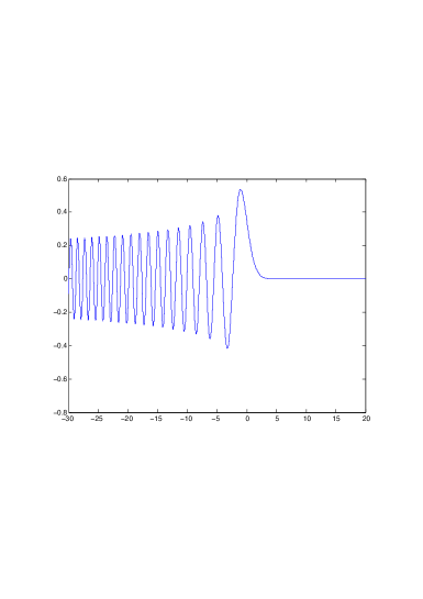
Figure 3. The Airy function.

7.1.1. Molecular dynamics for the Airy function

The eikonal equation corresponding to (7.2) is

$$p^{2}+x=0$$

with solutions for $x\leq 0$, which leads to the phase

(7.5) $$p=\theta^{\prime}(x)=\pm(-x)^{1/2}\,,\;\mbox{and}\;\;\theta(x)=\mp\frac{2}{3}(-x)^{3/2}\,.$$

We compute the Legendre transform

$${\theta}^{*}(p)=xp-\theta(x)$$

where by (7.5) and $-x=p^{2}$ we obtain

$${\theta}^{*}(p)=-p^{2}p+\frac{2}{3}p^{3}=-\frac{p^{3}}{3}\,.$$

We note that this solution is also obtained from the eikonal equation

$$p^{2}+\partial_{p}{\theta}^{*}(p)=0\,,$$

which is solved by

$${\theta}^{*}(p)=-p^{3}/3\,.$$

Thus we recover the relation for the Legendre transform $-xp+{\theta}^{*}(p)=-\theta(x)$.

7.1.2. Observables for the Airy function

The primary object of our analysis is an observable (a functional depending on $u$) rather than the solution $u(x)$ itself. Thus we first compute the observable evaluated on the solution obtained from the Airy function. In the following calculation we denote by $C$ a generic constant not necessarily the same at each occurrence,

(7.6) $$\begin{split}\int_{\mathbb{R}}g(x)|u(x)|^{2}dx&=C\int_{\mathbb{R}}g(x)\int_{\mathbb{R}}\int_{\mathbb{R}}e^{-iM^{1/2}(xp+p^{3}/3)}e^{iM^{1/2}(xq+q^{3}/3)}\,dq\,dp\,dx\\ &=C\int_{\mathbb{R}}\int_{\mathbb{R}}\hat{g}\left(M^{1/2}(p-q)\right)e^{iM^{1/2}(q^{3}/3-p^{3}/3)}\,dq\,dp\\ &=C\int_{\mathbb{R}}\int_{\mathbb{R}}\hat{g}\left(M^{1/2}(p-q)\right)e^{iM^{1/2}\left((q-p)^{3}/12+(q-p)(p+q)^{2}/4\right)}\,dq\,dp\\ &=C\int_{\mathbb{R}}\int_{\mathbb{R}}\hat{g}(\underbrace{-M^{1/2}\bar{q}}_{=t})\,e^{iM^{1/2}\left(\overline{q}^{3}/12+\overline{q}\,\overline{p}^{2}/4\right)}\overbrace{d\overline{q}d\overline{p}}^{\overline{q}=q-p,\,\overline{p}=p+q}\\ &=C\int_{\mathbb{R}}\int_{\mathbb{R}}\hat{g}(t)e^{-i\left(t^{3}/(12M)+t\,\overline{p}^{2}/4\right)}\,dt\,d\overline{p}\\ &=C\int_{\mathbb{R}}g*\mathrm{A}_{M}(\underbrace{-\overline{p}^{2}}_{=\partial_{p}{\theta}^{*}(\overline{p})=x})\,d\overline{p}\\ &=C\int_{-\infty}^{0}g*\mathrm{A}_{M}(x)|\partial_{x}p(x)|\,dx\,,\end{split}$$

where

(7.7) $$\mathrm{A}_{M}(x):=\left(\frac{M}{4}\right)^{1/3}\mathrm{A}\left(\left(\frac{M}{4}\right)^{1/3}x\right)\ \mbox{is the Fourier transform of $e^{-it^{3}/(12M)}$.}$$

Lemma 7.1.

The scaled Airy function $\mathrm{A}_{M}$ is an approximate identity in the following sense

(7.8) $$\|g*\mathrm{A}_{M}-g\|_{L^{2}(\mathbb{R})}\leq\frac{1}{12M}\|\partial^{3}_{x}g\|_{L^{2}(\mathbb{R})}\,.$$

Proof.

Plancherel’s Theorem implies

$$\begin{split}M\|g*\mathrm{A}_{M}-g\|_{L^{2}}&=M\|\hat{g}\hat{\mathrm{A}}_{M}-\hat{g}\|_{L^{2}}=\|\hat{g}(e^{ip^{3}/(12M)}-1)M\|_{L^{2}}\\ &\leq\frac{1}{12}\||p|^{3}\hat{g}\|_{L^{2}}=\frac{1}{12}\|\partial^{3}_{x}g\|_{L^{2}}\,.\end{split}$$

The inequality follows from $|e^{iy}-1|\leq|y|$ which holds for all $y\in\mathbb{R}$. $\Box$

The classical molecular dynamics approximation corresponding to the Schrödinger equation (7.2) is the Hamiltonian system

$$\dot{X}=p\,,\;\;\;\;\dot{p}=-\frac{1}{2}$$

with a solution $X_{t}=-t^{2}/4$ and the corresponding approximation of the observable

$$\frac{1}{T}\int_{0}^{T}g(X_{t})\,dt=\frac{1}{T}\int_{0}^{T}g(X_{t})\,\frac{dX_{t}}{\dot{X}_{t}}=\frac{1}{T}\int^{0}_{-T^{2}/4}g(x)\,\frac{dx}{|p(x)|}\,.$$

In this specific case the phase satisfies $|p(x)|=|x|^{1/2}$ and $|\partial_{x}p|=|x|^{-1/2}/2$, and hence the non-normalized density $|p|^{-1}$ is in this case equal to $2|\partial_{x}p|$. Equation (7.6) and Lemma 7.1 imply

$$|\int_{\mathbb{R}}g|u|^{2}\,dx-\int_{\mathbb{R}}g\partial_{x}p(x)\,dx|=\mathcal{O}(M^{-1})$$

and consequently for two different observables $g_{1}$ and $g_{2}$ we have that Schrödinger observables are approximated by the classical observables with the error $\mathcal{O}(M^{-1})$

(7.9) $$\frac{\int_{\mathbb{R}}g_{1}|u|^{2}\,dx}{\int_{\mathbb{R}}g_{2}|u|^{2}\,dx}-\frac{\int_{\mathbb{R}}g_{1}|\partial_{xx}\theta|\,dx}{\int_{\mathbb{R}}g_{2}|\partial_{xx}\theta|\,dx}=\mathcal{O}(M^{-1})\,,$$

using $\partial_{x}p(x)=\partial_{xx}\theta(x)$. The reason we compare two different observables with a compact support is that $\int_{\mathbb{R}}u^{2}(x)\,dx=\infty$ in the case of the Airy function.

We note that in (7.6) we used

$$\frac{1}{3}(q^{3}-p^{3})={\theta}^{*}(p)-{\theta}^{*}(q)=(p-q)\partial_{p}{\theta}^{*}\left(\frac{1}{2}(p+q)\right)+\frac{1}{3}{\partial^{3}{\theta}^{*}}\left(\frac{1}{2}(p+q)\right)\left(\frac{1}{2}(p-q)\right)^{3}$$

which in the next section is generalized to other caustics. For the Airy function there holds

$$\frac{1}{3}{\partial^{3}{\theta}^{*}\left(\frac{1}{2}(p+q)\right)}=-\frac{2}{3}\,.$$

7.2. A general Fourier integral ansatz

In order to treat a more general case with a caustic of the dimension $d$ we use the Fourier integral ansatz

(7.10) $$\Phi(X,x)=\int_{\mathbb{R}^{d}}\phi(X,x)e^{-iM^{1/2}\Theta({\check{X}},{\hat{X}},{\check{P}})}\,d{\check{P}}$$

and we write

$$\begin{split}X&=({\hat{X}},{\check{X}})\,,\;\;\;P=({\hat{P}},{\check{P}})\\ {{\check{X}}}\cdot{{\check{P}}}&=\sum_{j=1}^{d}{\check{X}}^{j}{\check{P}}^{j}\,,\;\;\;{{\hat{X}}}\cdot{{\hat{P}}}=\sum_{j=d+1}^{N}{\hat{X}}^{j}{\hat{P}}^{j}\\ \Theta({\check{X}},{\hat{X}},{\check{P}})&={{\check{X}}}\cdot{{\check{P}}}-{\theta}^{*}({\hat{X}},{\check{P}})\,,\end{split}$$

based on the Legendre transform

$${\theta}^{*}({\hat{X}},{\check{P}})=\min_{{\check{X}}}\left({{\check{X}}}\cdot{{\check{P}}}-\theta({\hat{X}},{\check{X}})\right)\,.$$

If the function ${\theta}^{*}({\hat{X}},{\check{P}})$ is not defined for all ${\check{P}}\in\mathbb{R}^{d}$, but only for ${\check{P}}\in\mathcal{U}\subset\mathbb{R}^{d}$ we replace the integral over $\mathbb{R}^{d}$ by integration over $\mathcal{U}$ using a smooth cut-off function $\chi({\check{P}})$. The cut-off function is zero outside $\mathcal{U}$ and equal to one in a large part of the interior of $\mathcal{U}$, see Section 7.2.3. The ansatz (7.10) is inspired by Maslov’s work  [25], although it is not the same since our amplitude function $\phi$ depends on $({\hat{X}},{\check{X}},x)$ but not on ${\check{P}}$. We emphasize that our modification consisting in having an amplitude function that is not dependent on ${\check{P}}$ is essential in the construction of the solution and for determining the accuracy of observables based on this solution.

7.2.1. Making the ansatz for a Schrödinger solution

In this section we construct a solution to the Schrödinger equation from the ansatz (7.10). The constructed solution will be an actual solution and not only an asymptotic solution as in  [25]. We consider first the case when the integration is over $\mathbb{R}^{d}$ and then conclude in the end that the cut-off function $\chi({\check{P}})$ can be included in all integrals without changing the property of the Fourier integral ansatz being a solution in the ${\check{X}}$-domain where ${\check{X}}=\nabla_{{\check{P}}}{\theta}^{*}({\hat{X}},{\check{P}})$ for some ${\check{P}}$ satisfying $\chi({\check{P}})=1$.

The requirement to be a solution means that there should hold

(7.11) $$\begin{split}0&=(\mathcal{H}-E)\Phi\\ &=\int_{\mathbb{R}^{d}}\left(\frac{1}{2}|\nabla_{{\hat{X}}}{\theta}^{*}({\hat{X}},{\check{P}})|^{2}+\frac{1}{2}|{\check{P}}|^{2}+V_{0}(X)-E\right)\phi(X,x)e^{-iM^{1/2}\Theta({\check{X}},{\hat{X}},{\check{P}})}\,d{\check{P}}\\ &\quad{}-\int_{\mathbb{R}^{d}}\left(iM^{-1/2}({\nabla_{{\hat{X}}}\phi}\cdot{\nabla_{{\hat{X}}}{\theta}^{*}}-{\nabla_{{\check{X}}}\phi}\cdot{{\check{P}}}+\frac{1}{2}\phi\Delta_{{\hat{X}}}{\theta}^{*})-(\mathcal{V}-V_{0})\phi+\frac{1}{2M}\Delta_{X}\phi\right)e^{-iM^{1/2}\Theta({\check{X}},{\hat{X}},{\check{P}})}\,d{\check{P}}\,.\end{split}$$

Comparing this expression to the previously discussed case of a single WKB-mode we see that the zero order term is now $\Delta_{{\hat{X}}}{\theta}^{*}$ instead of $\Delta_{X}\theta$ and that we have $-{\nabla_{{\check{X}}}\phi}\cdot{{\check{P}}}$ instead of ${\nabla_{{\check{X}}}\phi}\cdot{\nabla_{{\check{X}}}\theta}$. However, the main difference is that the first integral is not zero (only the leading order term of its stationary phase expansion is zero, cf. (9.1)). Therefore, the first integral contributes to the second integral. The goal is now to determine a function $F({\hat{X}},{\check{X}},{\check{P}})$ satisfying

(7.12) $$\begin{split}\int_{\mathbb{R}^{d}}&\left(\frac{1}{2}|\nabla_{{\hat{X}}}{\theta}^{*}|^{2}+\frac{1}{2}|{\check{P}}|^{2}+V_{0}(X)-E\right)e^{-iM^{1/2}\Theta({\check{X}},{\hat{X}},{\check{P}})}\,d{\check{P}}\\ &=iM^{-1/2}\int_{\mathbb{R}^{d}}F({\hat{X}},{\check{X}},{\check{P}})\,e^{-iM^{1/2}\Theta({\check{X}},{\hat{X}},{\check{P}})}\,d{\check{P}}\,,\end{split}$$

and verify that it is bounded.

Lemma 7.2.

There holds $F=F_{0}+F_{1}$ where

$$\begin{split}F_{0}&=\frac{1}{2}\sum_{i,j}\partial_{{\check{X}}^{i}{\check{X}}^{j}}V_{0}\left({\nabla_{{\check{P}}}{\theta}^{*}}({\check{P}})\right)\partial_{{\check{P}}^{j}{\check{P}}^{i}}{\theta}^{*}({\check{P}})\,,\\ F_{1}&=iM^{-1/2}\int_{0}^{1}\int_{0}^{1}\int_{\mathbb{R}^{d}}\sum_{i,j,k}t(1-t)\partial_{{\check{P}}^{k}}\left[\partial_{{\check{X}}^{i}{\check{X}}^{j}{\check{X}}^{k}}V_{0}\left({\nabla_{{\check{P}}}{\theta}^{*}}({\check{P}})+s\,t\,\delta{\theta}^{*}({\check{P}})\right)\partial_{{\check{P}}_{j}{\check{P}}_{i}}{\nabla_{{\check{P}}}{\theta}^{*}}({\check{P}})\right]\,dt\,ds\,.\\ \end{split}$$

Proof.

The function ${\theta}^{*}({\hat{X}},{\check{P}})$ is defined as a solution to the Hamilton-Jacobi (eikonal) equation

(7.13) $$\frac{1}{2}|\nabla_{{\hat{X}}}{\theta}^{*}({\hat{X}},{\check{P}})|^{2}+\frac{1}{2}|{\check{P}}|^{2}+V_{0}\left({\hat{X}},\nabla_{{\check{P}}}{\theta}^{*}({\hat{X}},{\check{P}})\right)-E=0$$

for all $({\hat{X}},{\check{P}})$. Consequently, the integral on the left hand side of (7.12) is

$$\int_{\mathbb{R}^{d}}\left(V_{0}({\hat{X}},{\check{X}})-V_{0}({\hat{X}},\nabla_{{\check{P}}}{\theta}^{*}({\hat{X}},{\check{P}})\right)e^{-iM^{1/2}\left({{\check{X}}}\cdot{{\check{P}}}-{\theta}^{*}({\hat{X}},{\check{P}})\right)}\,d{\check{P}}\,.$$

Let ${\check{P}}_{0}({\check{X}})$ be any solution to the stationary phase equation ${\check{X}}=\nabla_{{\check{P}}}{\theta}^{*}({\hat{X}},{\check{P}}_{0})$ and introduce the notation

$$\Theta^{\prime}({\check{X}},{\hat{X}},{\check{P}}):={\nabla_{{\check{P}}}{\theta}^{*}({\hat{X}},{\check{P}}_{0})}\cdot{{\check{P}}}-{\theta}^{*}({\hat{X}},{\check{P}})\,.$$

Then by writing a difference as $V(y_{1})-V(y_{2})=\int_{0}^{1}\partial_{y}V(y_{2}+t(y_{1}-y_{2}))dt\cdot(y_{1}-y_{2})$, identifying a derivative $\partial_{{\check{P}}_{i}}$ and integrating by parts the integral can be written

$$\begin{split}&\int_{\mathbb{R}^{d}}\left(V_{0}({\hat{X}},\nabla_{{\check{P}}}{\theta}^{*}({\hat{X}},{\check{P}}_{0}))-V_{0}({\hat{X}},\nabla_{{\check{P}}}{\theta}^{*}({\hat{X}},{\check{P}})\right)e^{-iM^{1/2}\Theta^{\prime}({\check{X}},{\hat{X}},{\check{P}})}\,d{\check{P}}\\ &=\int_{0}^{1}\int_{\mathbb{R}^{d}}\sum_{i}\partial_{{\check{X}}^{i}}V_{0}\left({\nabla_{{\check{P}}}{\theta}^{*}}({\check{P}})+t\,\left[{\nabla_{{\check{P}}}{\theta}^{*}}({\check{P}}_{0})-{\nabla_{{\check{P}}}{\theta}^{*}}({\check{P}})\right]\right)\times\\ &\qquad\times\left(\partial_{{\check{P}}^{i}}{\theta}^{*}({\check{P}}_{0})-\partial_{{\check{P}}^{i}}{\theta}^{*}({\check{P}})\right)e^{-iM^{1/2}\Theta^{\prime}({\check{X}},{\hat{X}},{\check{P}})}\,d{\check{P}}\,dt\\ &=-iM^{-1/2}\int_{0}^{1}\int_{\mathbb{R}^{d}}\sum_{i}\partial_{{\check{X}}^{i}}V_{0}\left({\nabla_{{\check{P}}}{\theta}^{*}}({\check{P}})+t\,\left[{\nabla_{{\check{P}}}{\theta}^{*}}({\check{P}}_{0})-{\nabla_{{\check{P}}}{\theta}^{*}}({\check{P}})\right]\right)\partial_{{\check{P}}_{i}}e^{-iM^{1/2}\Theta^{\prime}({\check{X}},{\hat{X}},{\check{P}})}\,d{\check{P}}\,dt\\ &=iM^{-1/2}\int_{0}^{1}\int_{\mathbb{R}^{d}}\sum_{i}\partial_{{\check{P}}_{i}}\partial_{{\check{X}}^{i}}V_{0}\left({\nabla_{{\check{P}}}{\theta}^{*}}({\check{P}})+t\,\left[{\nabla_{{\check{P}}}{\theta}^{*}}({\check{P}}_{0})-{\nabla_{{\check{P}}}{\theta}^{*}}({\check{P}})\right]\right)e^{-iM^{1/2}\Theta^{\prime}({\check{X}},{\hat{X}},{\check{P}})}\,d{\check{P}}\,dt\,.\end{split}$$

Therefore the leading order term in $F=:F_{0}+F_{1}$ is

$$\begin{split}F_{0}&:=\int_{0}^{1}\sum_{i,j}(1-t)\partial_{{\check{X}}^{i}{\check{X}}^{j}}V_{0}\left({\nabla_{{\check{P}}}{\theta}^{*}}({\check{P}})\right)\partial_{{\check{P}}^{j}{\check{P}}^{i}}{\theta}^{*}({\check{P}})\,dt\\ &=\frac{1}{2}\sum_{i,j}\partial_{{\check{X}}^{i}{\check{X}}^{j}}V_{0}\left({\nabla_{{\check{P}}}{\theta}^{*}}({\check{P}})\right)\partial_{{\check{P}}^{j}{\check{P}}^{i}}{\theta}^{*}({\check{P}})\,.\end{split}$$

Denoting $\delta{\theta}^{*}({\check{P}})={\nabla_{{\check{P}}}{\theta}^{*}}({\check{P}}_{0})-{\nabla_{{\check{P}}}{\theta}^{*}}({\check{P}})$ the remainder becomes

$$\begin{split}&-iM^{-1/2}\int_{0}^{1}\int_{\mathbb{R}^{d}}\sum_{i,j}\left[\partial_{{\check{X}}^{i}{\check{X}}^{j}}V_{0}\left({\nabla_{{\check{P}}}{\theta}^{*}}({\check{P}})\right)-\partial_{{\check{X}}^{i}{\check{X}}^{j}}V_{0}\left({\nabla_{{\check{P}}}{\theta}^{*}}({\check{P}})+t\,\delta{\theta}^{*}({\check{P}})\right)\right]\\ &\qquad\times(1-t)\partial_{{\check{P}}^{j}{\check{P}}^{i}}{\theta}^{*}({\check{P}})\,e^{-iM^{1/2}\Theta^{\prime}({\check{X}},{\hat{X}},{\check{P}})}\,d{\check{P}}\,dt\\ &=iM^{-1/2}\int_{0}^{1}\int_{0}^{1}\int_{\mathbb{R}^{d}}\sum_{i,j,k}t(1-t)\partial_{{\check{X}}^{i}{\check{X}}^{j}{\check{X}}^{k}}V_{0}\left({\nabla_{{\check{P}}}{\theta}^{*}}({\check{P}})+s\,t\,\delta{\theta}^{*}({\check{P}})\right)\partial_{{\check{P}}^{j}{\check{P}}^{i}}{\theta}^{*}({\check{P}})\\ &\qquad\times\left(\partial_{{\check{P}}^{k}}{\theta}^{*}({\check{P}}_{0})-\partial_{{\check{P}}^{k}}{\theta}^{*}({\check{P}})\right)e^{-iM^{1/2}\Theta^{\prime}({\check{X}},{\hat{X}},{\check{P}})}\,d{\check{P}}\,dt\,ds\\ &=-\frac{1}{M}\int_{0}^{1}\int_{0}^{1}\int_{\mathbb{R}^{d}}\sum_{i,j,k}t(1-t)\partial_{{\check{P}}^{k}}\left[\partial_{{\check{X}}^{i}{\check{X}}^{j}{\check{X}}^{k}}V_{0}\left({\nabla_{{\check{P}}}{\theta}^{*}}({\check{P}})+s\,t\,\delta{\theta}^{*}({\check{P}})\right)\partial_{{\check{P}}^{j}{\check{P}}^{i}}{\theta}^{*}({\check{P}})\right]\\ &\qquad\times e^{-iM^{1/2}\Theta^{\prime}({\check{X}},{\hat{X}},{\check{P}})}\,d{\check{P}}\,dt\,ds\,,\end{split}$$

hence the function $F_{1}$ is purely imaginary and small

$$\begin{split}&F_{1}=iM^{-1/2}\int_{0}^{1}\int_{0}^{1}\int_{\mathbb{R}^{d}}\sum_{i,j,k}t(1-t)\partial_{{\check{P}}^{k}}\left[\partial_{{\check{X}}^{i}{\check{X}}^{j}{\check{X}}^{k}}V_{0}\left({\nabla_{{\check{P}}}{\theta}^{*}}({\check{P}})+s\,t\,\delta{\theta}^{*}({\check{P}})\right)\partial_{{\check{P}}_{j}{\check{P}}_{i}}{\nabla_{{\check{P}}}{\theta}^{*}}({\check{P}})\right]\,dt\,ds\,,\end{split}$$

and

(7.14) $$2\mathrm{Re}\,{F}=\sum_{i,j}\partial_{{\check{X}}^{i}{\check{X}}^{j}}V_{0}\left({\nabla_{{\check{P}}}{\theta}^{*}}({\check{P}})\right)\partial_{{\check{P}}^{j}{\check{P}}^{i}}{\theta}^{*}({\check{P}})\,.$$

$\Box$

The eikonal equation (7.13) and the requirement that $(\mathcal{H}-E)\Phi=0$ in (7.11) then imply that

(7.15) $$\begin{split}0&=\int_{\mathbb{R}^{d}}\left[iM^{-1/2}\left({\nabla_{{\hat{X}}}\phi}\cdot{\nabla_{{\hat{X}}}{\theta}^{*}}-{\nabla_{{\check{X}}}\phi}\cdot{{\check{P}}}+\frac{1}{2}\phi\left(\Delta_{{\hat{X}}}{\theta}^{*}-2F(X,{\check{P}})\right)\right)\right.\\ &\qquad\left.-(\mathcal{V}-V_{0})\phi+\frac{1}{2M}\Delta_{X}\phi\right]e^{-iM^{1/2}\Theta({\check{X}},{\hat{X}},{\check{P}})}\,d{\check{P}}\,.\end{split}$$

The Hamilton-Jacobi eikonal equation (7.13), in the primal variable $({\hat{X}},{\check{P}})$ with the corresponding dual variable $\hat{P},\check{X})$, can be solved by the characteristics

(7.16) $$\begin{split}\dot{{\hat{X}}}&={\hat{P}}\\ \dot{{\hat{P}}}&=-\nabla_{{\hat{X}}}V_{0}({\hat{X}},{\check{X}})\\ \dot{{\check{X}}}&=-{\check{P}}\\ \dot{{\check{P}}}&=\nabla_{{\check{X}}}V_{0}({\hat{X}},{\check{X}})\,,\end{split}$$

using the definition

$$\begin{split}\nabla_{{\hat{X}}}{\theta}^{*}({\hat{X}},{\check{P}})&={\hat{P}}\\ \nabla_{{\check{P}}}{\theta}^{*}({\hat{X}},{\check{P}})&={\check{X}}\,.\end{split}$$

The characteristics give

$$\frac{d}{dt}\phi={\nabla_{{\hat{X}}}\phi}\cdot{\nabla_{{\hat{X}}}{\theta}^{*}}-{\nabla_{{\check{X}}}\phi}\cdot{{\check{P}}}\,,$$

so that the Schrödinger transport equation becomes, as in (3.12),

(7.17) $$iM^{-1/2}\left(\dot{\phi}+\phi\frac{\dot{G}}{G}\right)=(\mathcal{V}-V_{0})\phi-\frac{1}{2M}\Delta_{X}\phi$$

and for $\psi=G\phi$

(7.18) $$iM^{-1/2}\dot{\psi}=(\mathcal{V}-V_{0})\psi-\frac{G}{2M}\Delta_{X}\frac{\psi}{G}$$

with the complex valued weight function $G$ defined by

(7.19) $$\frac{d}{dt}\log G_{t}=\frac{1}{2}\Delta_{{\hat{X}}}{\theta}^{*}(\hat{X}_{t},{\check{P}}_{t})-F(\hat{X}_{t},{\check{P}}_{t})\,.$$

This transport equation is of the same form as the transport equation for a single WKB-mode, with a modification of the weight function $G$.

Differentiation of the second equation in the Hamiltonian system (7.16) implies that the first variation $\partial{\check{P}}_{t}/\partial{\check{X}}_{0}$ satisfies

$$\frac{d}{dt}\left(\frac{\partial{\check{P}}_{t}^{i}}{\partial{\check{X}}_{0}}\right)=\sum_{j,k}\partial_{{\check{X}}^{i}{\check{X}}^{j}}V_{0}({\hat{X}},{\check{X}}_{t})\partial_{{\check{P}}^{j}{\check{P}}^{k}}{\theta}^{*}({\check{P}})\frac{\partial{\check{P}}_{t}^{k}}{\partial{\check{X}}_{0}}\,,$$

which by the Liouville formula (3.14) and the equality

$$2\mathrm{Re}\,{F}=\sum_{i,j}\partial_{\check{X}^{i}\check{X}^{j}}V_{0}\partial_{{\check{P}}^{j}{\check{P}}^{i}}{\theta}^{*}=\mathrm{Tr}\,(\sum_{j}\partial_{{\check{X}}^{i}{\check{X}}^{j}}V_{0}\partial_{{\check{P}}^{j}{\check{P}}^{k}}{\theta}^{*})$$

in (7.14) yields the relation,

(7.20) $$e^{-2\int_{0}^{t}\mathrm{Re}\,{F}\,dt^{\prime}}=C\,\left|\det\frac{\partial{\check{P}}_{t}}{\partial{\check{X}}_{0}}\right|\,,$$

for the constant $C:=|\det\frac{\partial{\check{X}}_{0}}{\partial{\check{P}}_{0}}|$. We use relation (7.20) to study the density in the next section.

Remark 7.3.

The conclusion in this section holds also when all integrals over $d{\check{P}}$ in $\mathbb{R}^{d}$ are replaced by integrals with the measure $\chi({\check{P}})\,d{\check{P}}$. Then there holds $2\mathrm{Re}\,{F}=\sum_{ij}\partial_{{\check{X}}^{i}{\check{X}}^{j}}\mathcal{V}\partial_{{\check{P}}^{i}}(\chi\partial_{{\check{P}}^{j}}{\theta}^{*})$. We use that the observable $g$ is zero when the cut-off function $\chi_{j}$ is not one, see Section 7.2.3. In Section 7.2.5 we show how to construct a global solution by connecting the Fourier integral solutions, valid in a neighborhood where $\det\partial(X)/\partial(P)$ vanishes (and $\chi({\check{P}})=1$), to a sum of WKB-modes, valid in neighborhoods where $\det\partial(P)/\partial(X)$ vanishes (and $\chi({\check{P}})<1$).

7.2.2. The Schrödinger density for caustics.

In this section we study the density generated by the solution

$$\Phi(X,x)=\int_{\mathbb{R}^{d}}\phi(X,x)\,e^{-iM^{1/2}\left({{\check{X}}}\cdot{{\check{P}}}-{\theta}^{*}({\hat{X}},{\check{P}})\right)}\,d{\check{P}}\,.$$

The analysis of the density generalizes the calculations for the Airy function in Section 7.1.2. We have, using the notation $\hat{{\tilde{g}}}$ for the Fourier transform of ${\tilde{g}}$ with respect to the ${\check{X}}$ variable, and by introducing the notation $\check{R}=\tfrac{1}{2}({\check{P}}+{\check{Q}})$ and $\check{S}={\check{P}}-{\check{Q}}$

(7.21) $$\begin{split}\int g(X)|\Phi(x,X)|^{2}\,dxdX&=\int\underbrace{g(X)\langle{\phi},{\phi}\rangle}_{=:{\tilde{g}}(X)}\,e^{iM^{1/2}({{\check{X}}}\cdot{{\check{P}}}-{\theta}^{*}({\hat{X}},{\check{P}}))}\,e^{-iM^{1/2}({{\check{X}}}\cdot{{\check{Q}}}-{\theta}^{*}({\hat{X}},{\check{Q}}))}\,d{\check{P}}\,d{\check{Q}}\,dX\\ &=\int\hat{{\tilde{g}}}({\hat{X}},M^{1/2}\check{S})\,e^{iM^{1/2}({\theta}^{*}({\hat{X}},{\check{Q}})-{\theta}^{*}({\hat{X}},{\check{P}}))}\,d{\check{P}}\,d{\check{Q}}\,d{\hat{X}}\\ &=\int\hat{{\tilde{g}}}({\hat{X}},M^{1/2}\check{S})\,e^{iM^{1/2}\frac{1}{6}({\check{S}}\cdot{\nabla_{{\check{P}}})^{3}{\theta}^{*}({\hat{X}},\check{R}}+\gamma\check{S}/2)}\times\\ &\qquad\times e^{iM^{1/2}{\check{S}}\cdot{\nabla_{{\check{P}}}{\theta}^{*}({\hat{X}},\check{R})}}\,d\check{S}\,d\check{R}\ d{\hat{X}}\\ &=\left(\frac{1}{2\pi}\right)^{d/2}M^{-1/2}\int{\tilde{g}}*\mathrm{A}_{M}\big{(}{\hat{X}},\underbrace{\nabla_{{\check{P}}}{\theta}^{*}({\hat{X}},\check{R}}_{={\check{X}}})\big{)}\,d\check{R}d{\hat{X}}\\ &=\left(\frac{1}{2\pi}\right)^{d/2}M^{-1/2}\int{\tilde{g}}*\mathrm{A}_{M}({\hat{X}},{\check{X}})\,\left|\det\frac{\partial({\check{P}})}{\partial({\check{X}})}\right|\,dX\,.\end{split}$$

In the convolution ${\tilde{g}}*\mathrm{A}_{M}$, the function $\mathrm{A}_{M}$, analogous to (7.7), is the Fourier transform of

$$e^{i\frac{1}{M}({\omega}\cdot{\nabla_{{\check{P}}})^{3}{\theta}^{*}({\hat{X}},{\check{P}})}}\Big{|}_{{\check{P}}=\check{R}+\gamma\omega}$$

with respect to $\omega\in\mathbb{R}^{d}$ and the integration in ${\check{X}}$ is with respect to the range of $\nabla_{{\check{P}}}{\theta}^{*}({\hat{X}},\cdot)$. As a next step we evaluate the Fourier transform and its derivatives at zero and obtain

$$\begin{split}&\int_{\mathbb{R}^{d}}\mathrm{A}_{M}({\check{X}})\,d{\check{X}}=1\,,\;\;\;\int_{\mathbb{R}^{d}}{\check{X}}^{i}\mathrm{A}_{M}({\check{X}})\,d{\check{X}}=0\,,\\ &\int_{\mathbb{R}^{d}}{\check{X}}^{i}{\check{X}}^{j}\mathrm{A}_{M}({\check{X}})\,d{\check{X}}=0\,,\;\;\;M\int_{\mathbb{R}^{d}}{\check{X}}^{i}{\check{X}}^{j}{\check{X}}^{k}\mathrm{A}_{M}({\check{X}})\,d{\check{X}}=\mathcal{O}(1).\\ \end{split}$$

Here we use that both differentiation with respect to $({\omega}\cdot{\nabla_{{\check{P}}}})^{3}$ and ${\theta}^{*}({\hat{X}},\check{R}+\gamma\omega)$ yield factors of $\omega$ which vanish. The vanishing moments of $\mathrm{A}_{M}$ imply that

(7.22) $$\|{\tilde{g}}*\mathrm{A}_{M}-{\tilde{g}}\|_{L^{2}(d{\check{X}})}=\mathcal{O}(M^{-1})$$

as in (7.8), so that up to $\mathcal{O}(M^{-1})$ error the convolution with $\mathrm{A}_{M}$ can be neglected.

7.2.3. Integration over a compact set in ${\check{P}}$

In the case when the integration is over $\mathcal{U}\subset\mathbb{R}^{d}$ instead of $\mathbb{R}^{d}$, we use a smooth cut-off function $\chi({\check{P}})$, which is zero outside $\mathcal{U}$ and restrict our analysis to the case when the smooth observable mapping ${\check{P}}\mapsto g({\hat{X}},\nabla_{{\check{P}}}{\theta}^{*}({\hat{X}},{\check{P}}))$ is compactly supported in the domain where $\chi$ is one. In this way $g({\hat{X}},\nabla_{{\check{P}}}{\theta}^{*}({\hat{X}},{\check{P}}))$ is zero when $\nabla_{{\check{P}}}\chi({\check{P}})$ is non zero. The integrand is thus equal to

$$(g(X)\ \langle{\phi},{\phi}\rangle)\chi({\check{P}})\chi({\check{Q}})$$

and we use the convergent Taylor expansion

$$\chi(\underbrace{\check{R}+M^{-1/2}\omega}_{{\check{P}}})\chi(\underbrace{\check{R}-M^{-1/2}\omega}_{{\check{Q}}})=\sum_{k=0}^{\infty}\frac{|\omega|^{2k}}{M^{k}}a_{k}(\check{R})\,.$$

Then the observable becomes

$$(2\pi)^{-d/2}M^{-1/2}\sum_{k=0}^{\infty}\int\left(a_{k}\,(M^{-1}\Delta_{{\check{X}}})^{k}{\tilde{g}}\right)*\mathrm{A}_{M}\left({\hat{X}},\nabla_{{\check{P}}}{\theta}^{*}({\hat{X}},\check{R})\right)\,d\check{R}\,d{\hat{X}}\,.$$

As in (7.22) we can remove the convolution with $\mathrm{A}_{M}$ by introducing an error $\mathcal{O}(M^{-1})$ and since for $k>0$ we have $a_{k}(\check{R})g({\hat{X}},\nabla_{{\check{P}}}{\theta}^{*}({\hat{X}},\check{R}))=0$ and $a_{0}=1$, we obtain the same observable as before

$$\begin{split}&\sum_{k=0}^{\infty}\int\left(a_{k}\,(M^{-1}\Delta_{{\check{X}}})^{k}{\tilde{g}}\right)*\mathrm{A}_{M}\big{(}{\hat{X}},\nabla_{{\check{P}}}{\theta}^{*}({\hat{X}},\check{R})\big{)}\,d\check{R}\,d{\hat{X}}\\ &=\sum_{k=0}^{\infty}\int\left(a_{k}\,(M^{-1}\Delta_{{\check{X}}})^{k}{\tilde{g}}\right)\left({\hat{X}},\nabla_{{\check{P}}}{\theta}^{*}({\hat{X}},\check{R})\right)\,d\check{R}\,d{\hat{X}}\,+\mathcal{O}(M^{-1})\\ &=\int{\tilde{g}}\left({\hat{X}},\nabla_{{\check{P}}}{\theta}^{*}({\hat{X}},\check{R})\right)\,d\check{R}\,d{\hat{X}}\,+\mathcal{O}(M^{-1})\\ &=\int{\tilde{g}}({\hat{X}},{\check{X}})\,\left|\det\frac{\partial({\check{P}})}{\partial({\check{X}})}\right|\,dX\,+\mathcal{O}(M^{-1})\,.\end{split}$$

7.2.4. Comparing the Schrödinger and molecular dynamics densities

We compare the Schrödinger density to the molecular dynamics density generated by the continuity equation

$$0={\mathrm{div}}(\rho\nabla\theta)={\nabla\rho}\cdot{\nabla\theta}+\rho\,{\mathrm{div}}(\nabla{\theta})=\dot{\rho}+\rho\,{\mathrm{div}}(\nabla\theta)$$

which yields the density

$$e^{-\int{\mathrm{div}}(\nabla\theta)\,dt}\,.$$

We have $P=\nabla\theta$, so that $\tfrac{\partial(P)}{\partial(X)}=\partial_{XX}\theta$. The Liouville formula (3.14) implies the molecular dynamics density

(7.23) $$\begin{split}\rho_{{\mathrm{BO}}}=e^{-\int_{0}^{t}{\mathrm{div}}(\nabla\theta)\,dt^{\prime}}&=\det\frac{\partial X_{0,{\mathrm{BO}}}}{\partial X_{t,{\mathrm{BO}}}}\,.\end{split}$$

The observable for the Schrödinger equation has, by (7.21), the density

$$(g\langle{\phi},{\phi}\rangle)*\mathrm{A}_{M}\left|\det\frac{\partial({\check{P}})}{\partial({\check{X}})}\right|\,.$$

We want to compare it with the molecular dynamics density $\rho_{{\mathrm{BO}}}$. The convolution with $\mathrm{A}_{M}$ gives an error term of the order $\mathcal{O}(M^{-1})$, as in (7.8), and following the proof of Theorem 5.1 for a single WKB-state in Section 6 (now based on the Hamilton-Jacobi equation (7.13), the Schrödinger transport equation (7.17) and the definition of the weight $G$ in (7.19)), the amplitude function satisfies, by (7.18) and (7.19) and the Born-Oppenheimer approximation Lemma 6.2,

$$\langle{\phi},{\phi}\rangle=|G|^{2}\langle\psi,\psi\rangle=e^{\int 2\mathrm{Re}\,\,F-\Delta_{{\hat{X}}}{\theta}^{*}\,dt}+\mathcal{O}(M^{-1}),$$

so that by (7.20)

(7.24) $$\begin{split}(g\langle{\phi},{\phi}\rangle)*\mathrm{A}_{M}|\det\frac{\partial({\check{P}})}{\partial({\check{X}})}|&=(g\langle{\phi},{\phi}\rangle)|\det\frac{\partial({\check{P}})}{\partial({\check{X}})}|+\mathcal{O}(M^{-1})\\ &=g\,e^{\int 2\mathrm{Re}\,{F}-\Delta_{{\hat{X}}}{\theta}^{*}\,dt}\,|\det\frac{\partial({\check{P}})}{\partial({\check{X}})}|+\mathcal{O}(M^{-1})\\ &=g\,|\det\frac{\partial({\check{X}}_{0})}{\partial({\check{P}})}|\,|\det\frac{\partial({\hat{X}}_{0})}{\partial({\hat{X}})}|\,|\det\frac{\partial({\check{P}})}{\partial({\check{X}})}|+\mathcal{O}(M^{-1})\,,\\ &=g\,|\det\frac{\partial({\check{X}}_{0})}{\partial({\check{X}})}|\,|\det\frac{\partial({\hat{X}}_{0})}{\partial({\hat{X}})}|+\mathcal{O}(M^{-1})\,,\\ &=g\,|\det\frac{\partial(X_{0})}{\partial(X)}|+\mathcal{O}(M^{-1})\,.\end{split}$$

When we restrict the domain to $\mathcal{U}$ with the cut-off function $\chi$ as in Remark 7.3 we use the fact that $g({\hat{X}},\nabla_{{\check{P}}}{\theta}^{*}({\hat{X}},{\check{P}}))$ is zero when $\nabla_{{\check{P}}}\chi({\check{P}})$ is non zero and obtain the same. The representations (7.24) and (7.23) show that the density generated in the caustic case with a Fourier integral also takes the same form, to the leading order, as the molecular dynamics density and the remaining discrepancy is only due to ${\theta}^{*}={\theta}^{*}_{{\mathrm{S}}}$ and ${\theta}^{*}={\theta}^{*}_{{\mathrm{BO}}}$ being different. This difference is, as in the single mode WKB expansion, of size $\mathcal{O}(M^{-1})$ which is estimated by the difference in Hamiltonians of the Schrödinger and molecular dynamics eikonal equations. The estimate of the difference of the phase functions uses the Hamilton-Jacobi equation (7.13) for ${\theta}^{*}_{{\mathrm{S}}}({\hat{X}},{\check{P}})$ and a similar Hamilton-Jacobi equation for ${\theta}^{*}_{{\mathrm{BO}}}({\hat{X}},{\check{P}})$ with $V_{0}=\lambda_{{\mathrm{BO}}}+\mathcal{O}(M^{-1})$ replaced by $\lambda_{{\mathrm{BO}}}$. The difference in the weight functions $\log(|G({\hat{X}},{\check{P}})|^{-2})$ is estimated by the Hamilton-Jacobi equation

$$\left({\nabla_{{\hat{X}}}{\theta}^{*}_{{\mathrm{S}}}({\hat{X}},{\check{P}})}\cdot{\nabla_{{\hat{X}}}}-{\nabla_{{\check{X}}}V_{0}({\hat{X}},{\check{X}})}\cdot{\nabla_{{\check{P}}}}\right)\log|G_{{\mathrm{S}}}({\hat{X}},{\check{P}})|^{-2}-\Delta_{{\hat{X}}}{\theta}^{*}_{{\mathrm{S}}}(X,{\check{P}})+\mathrm{Re}\,{F}(X,{\check{P}})=0\,,$$

where $\mathrm{Re}\,{F}$ is given in (7.14), and by the similar Hamilton-Jacobi equation with $V_{0}=\lambda_{{\mathrm{BO}}}+\mathcal{O}(M^{-1})$ replaced by $\lambda_{{\mathrm{BO}}}$ and ${\theta}^{*}_{{\mathrm{S}}}$ by ${\theta}^{*}_{{\mathrm{BO}}}$.

7.2.5. A global construction coupling caustics with single WKB-modes

We use a Hamiltonian system to construct solutions to the Schrödinger equation. Given a set of initial points $X_{0}\in\mathbb{R}^{3N}$ the solution paths $\{(X_{t},P_{t})\in\mathbb{R}^{6N}{\,|\,}0\leq t<\infty,\,H(P_{0},X_{0})=E\}$ of the Hamiltonian system

$$\begin{split}\dot{X}_{t}&=\nabla_{P}H(P_{t},X_{t})\\ \dot{P}_{t}&=-\nabla_{X}H(P_{t},X_{t})\end{split}$$

with a smooth and bounded Hamiltonian $H(P,X)$ generate a $3N$-dimensional manifold called Lagrangian manifold. The Lagrangian manifold defined by the tube of trajectories is defined by the phase function $\theta(X)$ that plays the role of a generating function of the Lagrangian manifold. Thus we seek a function $\theta:U\subset\mathbb{R}^{3N}\to\mathbb{R}$ such that $P_{t}=\nabla_{X}\theta(X_{t})$. We show that there exists a potential function $\theta$ by determining an equation that preserves the symmetry for the matrix $Q_{t}$, defined as $Q^{ij}(X):=\partial_{X^{j}}P^{i}(X)$ and $Q^{ij}_{t}:=Q^{ij}(X_{t})$. The relations $P^{i}_{t}=P^{i}(X_{t})$ and $Q_{t}^{ij}:=\partial_{X^{j}}P^{i}(X_{t})$ imply

$$\dot{P}^{i}_{t}=\frac{d}{dt}P^{i}(X_{t})=\sum_{j}\dot{X}^{j}_{t}\partial_{X^{j}}P^{i}_{t}=\sum_{j}\dot{X}^{j}_{t}Q^{ij}_{t}=\sum_{j}\partial_{P^{j}}H\big{(}P(X_{t}),X_{t}\big{)}Q_{t}^{ij}\,,$$

so that

$$\begin{split}\partial_{X^{k}}\dot{P}^{i}_{t}&=\partial_{X^{k}}\Big{(}\sum_{j}\partial_{P^{j}}H\big{(}P(X_{t}),X_{t}\big{)}Q_{t}^{ij}\Big{)}\\ &=\underbrace{\sum_{j}\dot{X}^{j}_{t}\partial_{X^{k}}Q^{ij}_{t}}_{=\sum_{j}\dot{X}^{j}_{t}\partial_{X^{k}X^{j}}P^{i}_{t}=\sum_{j}\dot{X}^{j}_{t}\partial_{X^{j}X^{k}}P^{i}_{t}=\dot{Q}^{ik}_{t}}+\sum_{j}\partial_{P^{j}P^{l}}H\big{(}P(X_{t}),X_{t}\big{)}\underbrace{\partial_{X^{k}}P^{l}}_{=Q^{lk}}Q^{ij}\\ &+\sum_{j}\partial_{P^{j}X^{k}}H\big{(}P(X_{t}),X_{t}\big{)}Q^{ij}_{t}\end{split}$$

and

$$\partial_{X^{k}}\dot{P}^{i}_{t}=-\partial_{X^{k}}\Big{(}\partial_{X^{i}}H\big{(}P(X_{t}),X_{t}\big{)}\Big{)}=-\partial_{X^{i}X^{k}}H\big{(}P(X_{t}),X_{t}\big{)}\Big{)}-\sum_{j}\partial_{X^{i}P^{j}}H\big{(}P(X_{t}),X_{t}\big{)}\underbrace{\partial_{X^{k}}P^{j}}_{=Q^{jk}_{t}}$$

together with the symmetry of $Q_{t}$ show that

(7.25) $$\begin{split}\dot{Q}_{t}^{ik}&=-\partial_{X^{i}X^{k}}H(P_{t},X_{t})-\sum_{j,l}\partial_{P^{j}P^{l}}H(P_{t},X_{t})Q_{t}^{kl}Q_{t}^{ij}\\ &\qquad-\sum_{j}\partial_{P^{j}X^{k}}H(P_{t},X_{t})Q^{ij}_{t}-\sum_{j}\partial_{P^{j}X^{i}}H(P_{t},X_{t})Q^{kj}_{t}\,.\end{split}$$

Since the Hamiltonian is assumed to be smooth it follows that the right hand side in (7.25) is symmetric and thus the matrix $Q_{t}$ remains symmetric if it is initially symmetric. Hence there exists a potential function $\theta(X)$ such that $P(X)=\nabla_{X}\theta(X)$ in simple connected domains where $Q$ is smooth. The function $Q$ may become unbounded due to the term $\partial_{P^{j}P^{l}}H\,Q^{kl}Q^{ij}$, even though $H$ has bounded third derivatives. Points $X_{t}$ at which $\left|\mathrm{Tr}\,(Q_{t})\right|=\infty$ satisfy, by Liouville’s theorem (see Section 3.1.3), $\left|\det\frac{\partial X_{0}}{\partial X_{t}}\right|=\infty$ and such points are called caustic points.

The same construction of a potential works for the local chart expressed as $X=X(P)$ instead of $P=P(X)$. In fact any new variable $\hat{X}$ (not including both $X^{i}$ and $P^{i}$ for any $i$), based on $3N$ of the $6N$ variables $(X,P)$, and the remaining variables $3N$ variables, $\hat{P}$, represent the same Hamiltonian system with the Hamiltonian $\hat{H}(\hat{P},\hat{X}):=H(P,X)$. The Lagrangian manifold is defined by $\hat{P}=\nabla_{\hat{X}}\hat{\theta}(\hat{X})$ in the local chart of $\hat{P}$-coordinates with the generating (potential) function $\hat{\theta}(\hat{X})$ defined in domains excluding caustics, i.e., where $\det\left|\tfrac{\partial\hat{X}_{0}}{\partial\hat{X}_{t}}\right|<\infty$. Maslov,  [25], realized that a Lagrangian manifold can be partitioned, by changing coordinates in the neighborhood of a caustic, into domains where $\hat{P}=\nabla_{\hat{X}}\hat{\theta}(\hat{X})$ is smooth. He used the generating (potential) functions $\hat{\theta}$ to construct asymptotic WKB solutions of Fourier integral type. A sketch of this general situation is depicted in Figure 4. In previous sections we have described global construction of solutions in a simpler case without caustics, i.e., $P_{t}=\nabla_{X}\theta(X_{t})$ holds everywhere. In this section we describe the global construction of WKB solutions in the general case when caustics are present.

Figure 4. The left figure depicts a graph of the molecular dynamics potential $\lambda(X)$ in the case which exhibits caustics at $X=a$ and $X=b$ for a given energy $E$. The right figure shows a general case of the Lagrangian manifold with two caustic points $X=a$ and $b$ and its covering with charts $\mathcal{U}_{i}$. In the charts $\mathcal{U}_{i}$, $i=2,4$ the manifold is defined by $P=\nabla_{X}\theta_{i}(X)$ and the solution to Schrödinger equation is constructed by simple WKB modes. The caustics belong to the charts $\mathcal{U}_{i}$, $i=1,3$ and in this case the manifold is defined by $X=\nabla_{X}\theta_{i}(P)$ and the solutions are given by the Fourier integrals.

We see that the weight function $G$, in (3.14), based on a single WKB-mode (3.1) blows up at caustics, where $\det(\partial({\check{X}})/\partial({\check{P}}))=0$, and that the weight function $G$ in (7.17) for the Fourier integral (7.10) blows up at points where $\det(\partial({\check{P}})/\partial({\check{X}}))$ vanishes. Therefore, in neighborhoods around caustic points we need to use the representation ${\theta}^{*}({\hat{X}},{\check{P}})$ of the phase based on the Fourier integrals, while around points where $\det(\partial({\check{P}})/\partial({\check{X}}))$ vanishes we apply the representation $\theta({\hat{X}},{\check{X}})$ based on the Legendre transform, as pointed out by Maslov in  [25] and described in the simplifying setting of the harmonic oscillator in  [11].

One way to make a global construction of a WKB solution, which is slightly different than in  [25], is to use the characteristics and a partition of the phase-space as follows, also explained constructively by the numerical algorithm 3 in the next section. Start with a Fourier integral representation in a neighborhood $\mathcal{U}$ of a caustic point, which gives a representation of the Schrödinger solution $\Phi$ in $\mathcal{U}$. Then we use the stationary phase expansion, see Section 9, to find an asymptotic approximation $\tilde{\Phi}$ (accurate to any order $\bar{N}\in\mathbb{N}$) at the boundary points ${\check{X}}$ of $\mathcal{U}$ as a sum of single WKB-modes with phase functions $\theta_{j}$

$$\int_{\mathbb{R}^{d}}\chi({\check{P}})e^{-iM^{1/2}({{\check{X}}}\cdot{{\check{P}}}-{\theta}^{*}({\hat{X}},{\check{P}}))}\,d{\check{P}}=\sum_{j}e^{-iM^{1/2}\theta_{j}(X)}\phi_{j}(X)+\mathcal{O}(M^{-\bar{N}})$$

where each phase function $\theta_{j}(X):={{\check{X}}}\cdot{{\check{P}}_{X,j}}-{\theta}^{*}({\hat{X}},{\check{P}}_{X,j})$ corresponds to a branch of the boundary and the index $j$ corresponds to different solutions ${\check{P}}_{X,j}$ of the stationary phase equation ${\check{X}}=\nabla_{{\check{P}}}{\theta}^{*}({\hat{X}},{\check{P}}_{X})$. The single WKB-modes $\phi(x,X)e^{iM^{1/2}\theta(X)}$ are then constructed along the characteristics to be Schrödinger solutions in a domain around the point where $\det(\partial({\check{P}})/\partial({\check{X}}))$ vanishes, following the construction in Theorem 3.1 using the initial data of $\tilde{\Phi}$ at $\partial\mathcal{U}$. We note that the tiny error of size $\mathcal{O}(M^{-\bar{N}})$ that we make in the initial data for $\phi$ also yields a tiny perturbation error in $\phi$ of size $\mathcal{O}(M^{-\bar{N}})$ along the path, due to the assumption of the finite hitting times. A small error we make in the expansion therefore leads to a negligible error in the Schrödinger solution and the corresponding density.

When a characteristic leaves the domain and enters another region around a caustic we again use the stationary phase method at the boundary to give initial data for $(X,P,\phi,G)$. When the characteristic finally returns to the first boundary $\partial\mathcal{U}$, there is a compatibility condition to have a global solution, by having the incoming final phase equal to the initial phase function in $\mathcal{C}^{1}$. We can think of this as trying to find a co-dimension one surface $I$ in $\mathbb{R}^{3N}$ where the incoming and outgoing phases are equal. First to have one point where they agree is possible if we restrict the possible solutions to a discrete set of energies $E$, i.e., the eigenvalues, and therefore the compatibility condition is called a quantization condition. Then, having one point where the difference of the two phase function is zero, we can combine this with the assumption that the Lagrangian manifold generated by the characteristics path $(X_{t},P_{t})$ is continuous: the two phases have the same gradient on $I$, since $(X,P)=(X,\nabla_{X}\theta(X))=\Big{(}\big{(}\hat{X},\nabla_{\check{P}}\theta^{*}(\hat{X},\check{P})\big{)},\big{(}\nabla_{\hat{X}}\theta^{*}(\hat{X},\check{P}),\check{P}\big{)}\Big{)}$ so the phases are $\mathcal{C}^{1}$. In this way we define the $(X,P,\phi,G)$ globally, for the eigenvalue energies $E$. To evaluate observables we use a partition of unity to restrict the observable to a domain with a single representation, either a Fourier integral representation for a caustic or a single WKB-mode when $\det(\partial({\check{P}})/\partial({\check{X}}))=0$.

8. Numerical examples

In order to demonstrate the presented theory we consider two different low dimensional Schrödinger problems. For both of these problems we show that there exists a Schrödinger eigenfunction density which converges weakly to the corresponding molecular dynamics density as $M\to\infty$ with a convergence rate within the upper bound predicted in the theoretical part of this paper.

8.1. Example 1: A single WKB state

The first problem we consider is the time-independent Schrödinger equation

(8.1) $$\mathcal{H}\Phi:=\left(-\frac{1}{2M}\partial_{XX}+\overline{\mathcal{V}}\right)\Phi=E\Phi$$

with heavy coordinate $X\in(-\pi,\pi]$ and two-state light coordinate $x\in\{x_{-},x_{+}\}$. Periodicity is assumed over the heavy coordinate, $\Phi(X,x)=\Phi(X+2\pi,x)$, and the potential operator $\overline{\mathcal{V}}$ is defined by the matrix

(8.2) $$\overline{\mathcal{V}}(X)=\left[\begin{array}[]{cc}V(X)&\tfrac{1}{2}V(X)e(X)+c\\ \tfrac{1}{2}V(X)e(X)+c&0\end{array}\right]\,,$$

where we have chosen $V(X)=-2\cos(X)+\cos(4X)$, $e(X)=1+X^{2}$ and $c$ to be a non-negative constant relating to the size of the spectral gap of $\overline{\mathcal{V}}$. The action $\overline{\mathcal{V}}\Phi$ is thus defined by

$$(\overline{\mathcal{V}}\Phi)(X,\cdot)\equiv\overline{\mathcal{V}}(X)\left(\begin{array}[]{c}\Phi(X,x_{-})\\ \Phi(X,x_{+})\end{array}\right)\,.$$

For each $X$ the potential matrix (8.2) gives rise to the eigenvalue problem

$$\overline{\mathcal{V}}(X)\upsilon=\lambda_{\pm}(X)\upsilon$$

with the eigenvalues

$$\lambda_{\pm}(X)=\frac{1}{2}\left(V(X)\pm\mathrm{Sgn}(X)\sqrt{V(X)^{2}+4\big{(}V(X)e(X)/2+c\big{)}^{2}}\right)\,,$$

where $\mathrm{Sgn}(X)=\pm 1$ as defined below. When constructing the molecular dynamics density for this problem

$$\rho_{{\mathrm{MD}}}(X)=\frac{C}{\sqrt{2(E-\lambda(X))}}\,,$$

one has to determine on which of the two eigenfunctions $\lambda_{\pm}$ to base this density. When $c=0$ the difficulty that the eigenvalue functions $\lambda_{+}$ and $\lambda_{-}$ can cross is added to the problem. In order to determine the continuation of eigenvalue functions at the crossings we introduce a function $\mathrm{Sgn}(X)$ which is a sign function with $\mathrm{Sgn}(-\pi)=1$ that changes sign at points where

$$V(X)^{2}+4\left(\frac{1}{2}V(X)e(X)+c\right)^{2}=0\,.$$

Since this situation can only occur when $c=0$, it is possible to set

$$\mathrm{Sgn}(X):=\mathrm{sgn}(V(-\pi))\mathrm{sgn}(V(X))\,.$$

See Figure 5 for a typical eigenvalue function crossing, which makes the function $\lambda_{\pm}:\mathbb{R}\rightarrow\mathbb{R}$ smooth (in contrast to the choice $\mathrm{Sgn}\equiv 1$).

To solve (8.1) numerically, we use the finite difference method to discretise the operator $\mathcal{H}$ on a grid $\{X_{j}\}_{j=1}^{N}\times\{x_{-},x_{+}\}$ with the step-size $h=2\pi/N$ and $X_{j}=jh$. The discrete eigenvalue problem

$$\mathcal{H}^{(h)}\Upsilon_{j}=E_{j}\Upsilon_{j}$$

is solved for the 10 eigenvalues being closest to the fixed energy $E$ and a molecular dynamics approximation of the eigensolution is constructed by

$$\Phi_{{\mathrm{MD}}}(X,x):=\sqrt{\rho_{{\mathrm{MD}}}(X)}\,e^{iM^{1/2}\Theta(X)}\upsilon(X,x)\,,$$

where $\upsilon(X,\cdot)$ is one of the eigenvectors of $\overline{\mathcal{V}}(X)$ and

(8.3) $$\Theta(X):=\int_{0}^{X}\sqrt{2(E_{1}-\lambda(s))}\,ds$$

is approximated by a trapezoidal quadrature yielding $\Theta^{(h)}$. Thereafter a Schrödinger eigensolution $\Phi^{(h)}$ which is close to the molecular dynamics eigensolution is obtained by projecting $\Phi_{MD}$ onto the subspace spanned by $\{\Upsilon\}_{j=1}^{\bar{J}}$ as described in Algorithm 2. By denoting $\rho_{\Phi^{(h)}}(X)=\langle{\Phi^{(h)}},{\Phi^{(h)}}\rangle$ and $\rho_{{\mathrm{MD}}}(X)=\langle{\Phi_{{\mathrm{MD}}}},{\Phi_{{\mathrm{MD}}}}\rangle$, the observables $g_{1}(X)=X^{2}$ and $g_{2}(X)=V(X)$ are used to compute the convergence rate of

(8.4) $$\left|\frac{\int_{-\pi}^{\pi}g_{i}(X)\rho_{{\mathrm{MD}}}(X)\,dX-\int_{-\pi}^{\pi}g_{i}(X)\rho_{\Phi^{(h)}}(X)\,dX}{\int_{-\pi}^{\pi}g_{i}(X)\rho_{{\mathrm{MD}}}(X)\,dX}\right|\,,$$

as $M$ increases. Further details of the numerical solution idea are described in Algorithm 1.

Plots of the results for the test case with the spectral gap $c=5$ and $E=0$, and for the test case with crossing eigenvalue functions when $c=0$ and $E=1.2$ are given below. Most noteworthy is Figure 8, which demonstrates that the obtained convergence rate for (8.4) is $\mathcal{O}(M^{-1})$ for both scenarios.

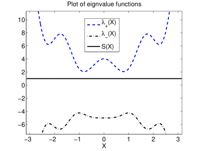
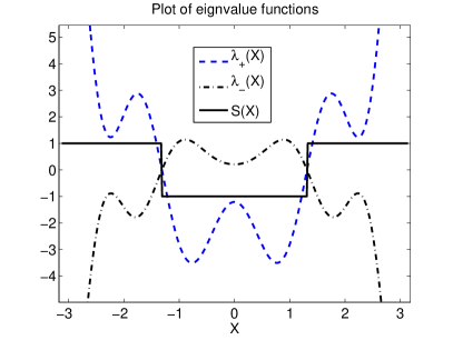
Figure 5. Left plot: Eigenvalue functions when $c=5$. There is a spectral gap which makes the sign function constant $S=1$. Right plot: Eigenvalue functions when $c=0$. The eigenvalue functions exhibit crossing, consequently the function $S$ changes its sign from $\pm 1$ to $\mp 1$ at the crossing points.

Algorithm 1 Algorithm for problems in Example 1

  Input: Energy $E$; potential functions $V$, $e$ and $c$; mass $M$; number of grid points $N$ and grid $\{X_{i}\}_{i=1}^{N}$.

  Output: Schrödinger projection density $\rho_{\Phi^{(h)}}$.

  1. Construct the discrete operator $\mathcal{H}^{(h)}$ from (8.1) using finite differences and solve the eigenvalue problem

$$\mathcal{H}^{(h)}\Upsilon_{i}=E_{i}\Upsilon_{i}$$

for the 10 eigenvalues being closest to $E$ by using MATLAB eigs(H,10,E).

  2. Sort the eigenvalues and eigenvectors by distance from $E$ and keep only the $E_{i}$s which are less than $M^{-1/2}$ away from $E$. Let $\bar{J}$ be the number of kept eigenvalues and $E_{0}$ the eigenvalue closest to $E$.

  3.

  for $i=1$ to $N$ do

     Solve the eigenvalue problem

$$\overline{\mathcal{V}}(X_{i},\cdot)\upsilon_{\pm}(X_{i},\cdot)=\lambda_{\pm}(X_{i})\upsilon_{\pm}(X_{i},\cdot)\,,$$

where $\overline{\mathcal{V}}$ is the matrix defined in (8.2).

  end for

  4. Construct the molecular dynamics density according to the formula

$$\rho_{{\mathrm{MD}}}(X)=\frac{\left(E_{0}-\lambda(X)\right)^{-1/2}}{\int_{[0,2\pi]}\left(E_{0}-\lambda(X)\right)^{-1/2}\,dX}\,,$$

where we choose $\lambda(X)$ above from the two eigenvalues $\lambda_{\pm}(X)$ by the criterion that the eigenvalue chosen must fulfil $\|\lambda\|_{\infty}<E_{0}$.

  5. Construct a discrete molecular dynamics approximation to the eigenfunction

(8.5) $$\Phi_{{\mathrm{MD}}}(X,x)=\sqrt{\rho_{{\mathrm{MD}}}(X)}e^{iM^{1/2}\Theta(X)}\upsilon(X,x)\,,$$

where $\upsilon(X,x)$ is one of the eigenvectors $\upsilon_{\pm}$,

(8.6) $$\Theta(X):=\int_{0}^{X}\sqrt{2(E_{1}-\lambda(s))}\,ds\,,$$

and we approximate $\Theta$ by a trapezoidal quadrature $\Theta^{(h)}$.

  6. Project the molecular dynamics solution $\Phi_{{\mathrm{MD}}}$ onto the eigenspace $\{\Upsilon_{i}\}_{i=1}^{\bar{J}},\ \bar{J}\leq 10$ by Algorithm 2 to obtain a projection solution $\Phi^{(h)}$.

  7. Derive the Schrödinger projection density by

  for $i=1$ to $N$ do

     

$${\rho_{\Phi^{(h)}}}(X_{i})=|\Phi^{(h)}(X_{i},x_{-})|^{2}+|\Phi^{(h)}(X_{i},x_{+})|^{2}\,,$$

  end for

  and scaling $\rho_{\Phi^{(h)}}=\rho_{\Phi^{(h)}}/\|\rho_{\Phi^{(h)}}\|$.

Algorithm 2 Projection algorithm

  Input: Mass $M$; wave solution $\Phi$; eigenvalues $\{E_{i}\}_{i=1}^{\bar{J}}$ and corresponding eigenvectors $\{\Upsilon_{i}\}_{i=1}^{\bar{J}}$.

  Output: Schrödinger projection wave solution $\Phi^{(h)}$.

  1. Organize eigenvalues by multiplicity by a numerical approximation. Construct a $\bar{J}\times\bar{J}$, zero matrix $A$ which keeps track of multiplicity relations as follows:

  for $i=1$ to $\bar{J}$ do

     for $j=i$ to $\bar{J}$ do

        if $|E_{i}-E_{j}|<M^{-3/4}$  then

           Consider eigenvalues equal since the expected spectral gap is $\mathcal{O}(M^{-1/2})$, and store this relation by

           if $A_{kj}=0$ for all $k<i$ then

              Set $A_{ij}=1$.

           end if

        end if

     end for

  end for

  2. For vectors $b\in\{0,1\}^{\bar{J}}$, define the projection

$$\Phi^{(h,b)}:=\sum_{j,k=1}^{\bar{J}}b_{k}A_{k,j}\langle\!\langle\Phi,\Upsilon_{j}\rangle\!\rangle\Upsilon_{j}$$

and, letting $\rho$ and $\rho_{\Phi^{(h,b)}}$ denote the densities generated by $\Phi$ and $\Phi^{(h,b)}$ respectively, set

$$b^{*}=\arg\min_{b\in\{0,1\}^{\bar{J}}}\|\rho-\rho_{\Phi^{(h,b)}}\|.$$

  3. Return the projection $\Phi^{(h)}:=\Phi^{(h,b^{*})}$.

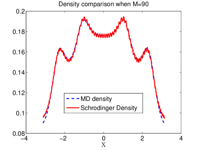
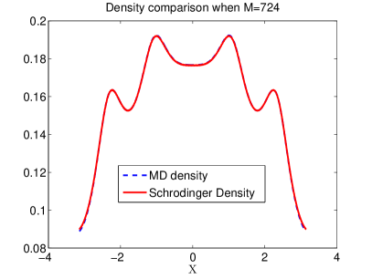
Figure 6. Plot of the MD density $\rho_{{\mathrm{MD}}}$ and the Schrödinger projection density $\rho_{\Phi^{(h)}}$ in the case $c=5$ and $E=0$ for the two different masses $M=90$ (left plot) and $M=724$ (right plot) illustrating the convergence of the densities.

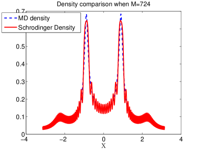
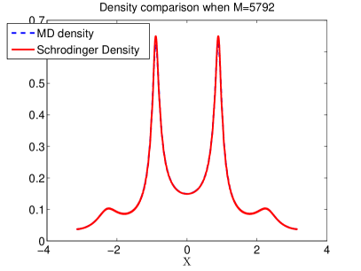
Figure 7. Plot of the MD density $\rho_{{\mathrm{MD}}}$ and Schrödinger projection density $\rho_{\Phi^{(h)}}$ in the case $c=0$ and $E=1.2$ for the two different masses $M=724$ (left plot) and $M=5792$ (right plot).

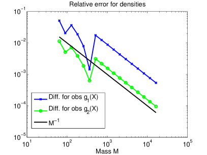
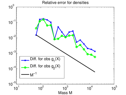
Figure 8. Left plot: Plot of the observable density errors given in (8.4) with an eigenvalue gap, when $c=5$ and $E=0$. Right plot: Plot of the observable density errors given in (8.4) with an eigenvalue crossing, when $c=0$ and $E=1.2$.

8.2. Example 2: A caustic state

Next, we consider the one dimensional, time independent, periodic Schrödinger equation

(8.7) $$\left(-\frac{1}{2M}\partial_{XX}+V\right)\Phi=E\Phi\,,\;\;\;X\in(-2\sqrt{E},2\sqrt{E})$$

with $V(X)=X^{2}$ and $E=1$. The eikonal equation corresponding to (8.7) is

(8.8) $$\frac{1}{2}{P^{2}}+V(X)=E\,.$$

As in Example 1, we would like to use the eikonal equation to construct a numerical approximate solution of (8.7) whose density converges weakly as $M\to\infty$ to the density generated from a solution of (8.7). The molecular dynamics density corresponding to this eikonal equation becomes by (3.19) $\rho_{{\mathrm{BO}}}=C(E-V(X))^{-1/2}$. The density $\rho_{{\mathrm{BO}}}$ goes to infinity at the caustics $X=V^{-1}(E)=\pm\sqrt{E}$ and the approach in Example 1 does not work directly. We will instead construct the numerical approximate solution using the stationary phase method as outlined below based on the WKB Fourier integral ansatz.

By the Legendre transform

$${\theta}^{*}(P)=\min_{X}\big{(}XP-\theta(X)\big{)}$$

an invertible mapping between the momentum and position coordinates fulfilling $X=\nabla_{P}{\theta}^{*}(P)$ is constructed. Using equation (8.8), one sees that $\nabla_{P}{\theta}^{*}(P)=V^{-1}(E-P^{2}/2)$. Since ${\theta}^{*}(0)=0$, one can derive that for this particular choice of $V$

$${\theta}^{*}(P)=\int_{0}^{P}\sqrt{E-s^{2}/2}\,ds=\frac{E}{\sqrt{2}}\left[\sin^{-1}\left(\frac{P}{\sqrt{2E}}\right)+\frac{P}{\sqrt{2E}}\sqrt{1-\frac{P^{2}}{2E}}\right].$$

In neighbourhoods of the caustics $[-2E^{1/2},-X_{0})$ and $(X_{0},2E^{1/2}]$, we construct the approximate solution by

$$\Phi(X)=\frac{u(X)}{\sqrt{|\nabla_{X}V(X)|}}$$

where $u$ is the inverse Fourier transform

$$u(X):=\int_{-2\sqrt{E}}^{2\sqrt{E}}e^{iM^{1/2}(-XP+{\theta}^{*}(P))}\,dP$$

and $X_{0}\in(-V^{-1}(E),V^{-1}(E))$ is a value yet to be chosen. In the region $(-X_{0},X_{0})$ the approximate solution is constructed by

(8.9) $$\Phi(X)=C\frac{\overline{u}(X)}{(E-V(X))^{1/4}}\,.$$

Here

(8.10) $$\overline{u}(X):=e^{-iM^{1/2}\theta(X)}\psi_{+}+e^{iM^{1/2}\theta(X)}\psi_{-}\,,$$

with, according to the Legendre transform, $\theta(X):=X\sqrt{2(E-V(X))}-{\theta}^{*}\left(\sqrt{2(E-V(X))}\right)$ and $\psi_{\pm}$ determined by the stationary phase method:

1. Set $P(p)=P_{0}+p$ with $P_{0}=\sqrt{2(E-V(X_{0}))}$ and let

   $$Y(p):=\mathrm{sgn}(p)\sqrt{2\frac{-X(P_{0}+p)+{\theta}^{*}(P_{0}+p)+\theta(X_{0})}{\partial_{PP}{\theta}^{*}(P_{0})}}\,,$$

   using

   (8.11) $$\theta(X):=X\sqrt{2(E_{0}-V(X))}-{\theta}^{*}\left(\sqrt{2(E_{0}-V(X))}\right)\,,$$

   and determine its inverse $p(Y)$ in a neighbourhood of $Y=0$ by computing $(p_{i},Y(p_{i}))$ on a grid around $p=0$ and, for $k\geq 3$, fit a $3k+1$th degree polynomial to the values $(Y(p_{i}),p_{i})$ using the method of least squares.

2. Evaluate the stationary phase expansion

   (8.12) $$\begin{split}u(X_{0})&=\sum_{p_{0}=\pm\sqrt{2(E-V(X_{0}))}}e^{i\pi\mathrm{sgn}(\partial_{PP}{\theta}^{*}(P_{0}))/4}\left[\left|\frac{1}{2}\partial_{PP}{\theta}^{*}(P_{0})\right|^{-1/2}e^{-iM^{1/2}\theta(X_{0})}\right.\\ &\qquad\times\left.\sum_{j=0}^{k}\frac{M^{-j/2}}{j!}\left(i\left(\frac{1}{2}\partial_{PP}{\theta}^{*}(P_{0})\right)^{-1}\partial_{YY}\right)^{j}|\partial_{Y}p|\right|_{Y=0}+\mathcal{O}(M^{-j/2})\Bigg{]}\end{split}$$

   to obtain

   $$u(X_{0}^{-})=e^{iM^{1/2}\theta(X_{0})}(\psi_{+}+\mathcal{O}(M^{-k/2}))+e^{-iM^{1/2}\theta(X_{0})}(\psi_{-}+\mathcal{O}(M^{-k/2}))\,,$$

   where

   $$\psi_{\pm}:=e^{i\pi\mathrm{sgn}(\partial_{PP}{\theta}^{*}(\pm P_{0}))/4}\left|\frac{1}{2}\partial_{PP}{\theta}^{*}(\pm P_{0})\right|^{-1/2}\sum_{k=0}^{3}\frac{M^{-k/2}}{k!}\left(i\left(\frac{\partial_{PP}{\theta}^{*}(\pm p_{0})}{2}\right)^{-1}\partial_{YY}\right)^{k}|\partial_{Y}p|\Big{|}_{Y=0}.$$

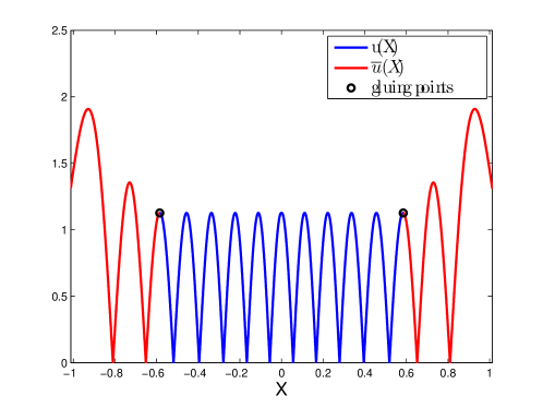
Figure 9. Plot illustrating the gluing procedure of the functions $u(X)$ and $\overline{u}(X)$ at the points $\pm X_{0}$.

The constant $C$ in (8.9) is chosen so that the wave solution parts are continuous at the gluing point, $\Phi(\pm X_{0}^{-})=\Phi(\pm X_{0}^{+})$. It is most easy to determine $C$ when $X_{0}$ is chosen so that $|u(X_{0})|$ is at a local maximum; see Figure 9 for an illustration of the gluing procedure.

At the end a Schrödinger eigenfunction solution $\Phi^{(h)}$ is obtained by projecting $\Phi$ onto the space spanned by a set of eigensolutions to the discretized version of the Schrödinger problem, $\{\Upsilon_{j}\}_{j=1}^{\bar{J}}$, as is described in Algorithm 2.

Two convergence results are needed to make the method work. First, the density generated from the stationary phase based on the approxmiate solution $\rho(X):=|\Phi|^{2}(X)/\|\Phi\|_{2}^{2}$ must converge weakly to the Schrödinger projection based density $\rho_{\Phi^{(h)}}(X):=|\Phi^{(h)}|^{2}(X)/\|\Phi^{(h)}\|_{2}^{2}$ as $M\to\infty$; see Figure 10 for an illustration of how these functions converge. Second, $\rho_{\Phi^{(h)}}$ must converge to the molecular dynamics density $\rho_{{\mathrm{MD}}}(X):=C(E-V(X))^{-1/2}$ as $M$ increases; see Figure 11.

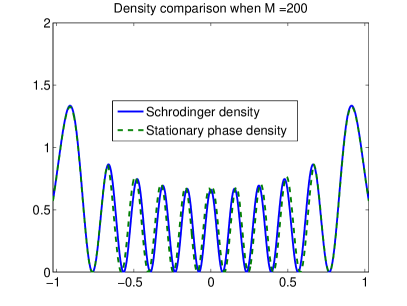
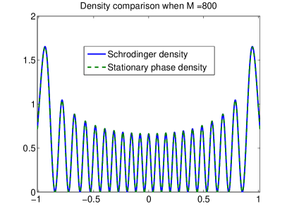
Figure 10. Comparison of the approximate solution based density $\rho$ and the Schrödinger projection based solution $\rho_{\Phi^{(h)}}$ for $M=200$ (left plot) and $M=800$ (right plot).

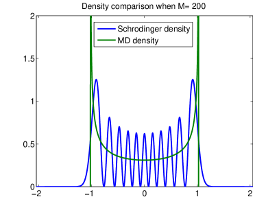
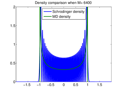
Figure 11. Comparision of the Schrödinger projection density $\rho_{\Phi^{(h)}}$ and the molecular dynamics density $\rho_{{\mathrm{MD}}}$ for $M=200$ (left plot) and $M=6400$ (right plot).

A numerical test of the convergence rate of

(8.13) $$\left|\frac{\int_{-2\sqrt{E_{0}}}^{2\sqrt{E_{0}}}g_{1}(X)\rho_{{\mathrm{MD}}}(X)\,dX}{\int_{-2\sqrt{E_{0}}}^{2\sqrt{E_{0}}}g_{2}(X)\rho_{{\mathrm{MD}}}(X)\,dX}-\frac{\int_{-2\sqrt{E_{0}}}^{2\sqrt{E_{0}}}g_{1}(X)\rho_{\Phi^{(h)}}(X)\,dX}{\int_{-2\sqrt{E_{0}}}^{2\sqrt{E_{0}}}g_{2}(X)\rho_{\Phi^{(h)}}(X)\,dX}\right|$$

as $M$ increases is illustrated in Figure 12 for the observables

(8.14) $$g_{1}(X)=\frac{(1.5-X)^{6}(1.5+X)^{6}(1+e^{-X^{2}})}{1.5^{12}}\;\text{ and }g_{2}(X)=\frac{(1.5-X)^{6}(1.5+X)^{6}(1-X^{2}+X^{4})}{1.5^{12}}\,.$$

Further details of the solution procedure in Exampe 2 are given in Algorithm 3.

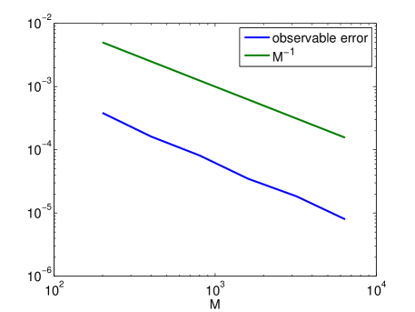
Figure 12. Convergence rate of (8.13) for the observables $g_{1}$ and $g_{2}$ as defined in (8.14).

Algorithm 3 Algorithm for Example 2

  Input: An energy $E$, an one-dimensional potential function $V$, mass $M$, Schrödinger equation (8.7).

  Output: The Schrödinger projection density $\rho_{\Phi^{(h)}}$.

  1. Identify the right caustic point $X_{+}>0$ satisfying $X_{+}=V^{-1}(E)$. For a fixed $E\in\mathbb{R}$, consider the periodic eigenvalue problem. Solve (8.7) numerically by constructing the discretised operator form of $-(2M)^{-1}\partial_{XX}+V$ using finite differences and denoted $\mathcal{H}^{(h)}$, and solve the eigenvalue problem

(8.15) $$\mathcal{H}^{(h)}P_{i}=E_{i}P_{i}$$

for the 10 eigenvalues closest to $E$ using the Matlab eigenvalue solver eigs(H,10,E). Let $E_{0}$ denote the eigenvalue closest to $E$ and consider from now on solving (8.7) for the energy $E_{0}$ and its corresponding eikonal equation $\tfrac{1}{2}P^{2}+V(X)=E_{0}$.

  2. Determine ${\theta}^{*}(P)$ by

$${\theta}^{*}(P)=\int_{0}^{P}\nabla_{P}{\theta}^{*}(p)\,dp$$

  3. Evaluate the Fourier integral

(8.16) $$u(X):=\int_{-2\sqrt{E}}^{2\sqrt{E}}e^{iM^{1/2}(-XP+{\theta}^{*}(P))}\,dP\,,\;\;|X|>X_{0}\,,$$

where $X_{0}$ is chosen as the smallest value $X>X_{+}/2$ such that $|u(X)|$ is at a local maximum, and for $|X|\leq X_{0}$ compute $\overline{u}$ by (8.10) using the stationary phase method.

  4. Construct the approximate solution

$$\Phi(X):=\begin{cases}C\overline{u}(X)(E_{0}-V(X))^{-1/4}&|X|\leq X_{0}\,,\\ u(X)/\sqrt{|\nabla_{X}V(X)|}&|X|\geq X_{0}\,,\end{cases}$$

with

$$C=\frac{u(X_{0})(E_{0}-V(X_{0}))^{1/4}}{\sqrt{|\nabla_{X}V(X_{0})|}\overline{u}(X_{0})}\,.$$

  5. Project $\Phi$ onto the eigenspace $\{\Upsilon_{i}\}_{i=1}^{\bar{J}},\ \bar{J}\leq 10$ by Algorithm 2 to obtain a projection solution $\Phi^{(h)}$ and compute its corresponding approximate density

$$\rho_{\Phi^{(h)}}=\frac{|\Phi^{(h)}|^{2}(X)}{\|\Phi^{(h)}\|_{2}^{2}}\,.$$

9. The stationary phase expansion

Consider the phase function ${{\check{X}}}\cdot{{\check{P}}}-{\theta}^{*}({\hat{X}},{\check{P}})$ and let ${\check{P}}_{0}({\hat{X}})$ be any solution to the stationary phase equation ${\check{X}}=\nabla_{{\check{P}}}{\theta}^{*}({\hat{X}},{\check{P}}_{0})$. We rewrite the phase function

$${{\check{X}}}\cdot{{\check{P}}}-{\theta}^{*}({\check{X}},{\check{P}})=\underbrace{{{\check{X}}}\cdot{{\check{P}}_{0}}-{\theta}^{*}({\check{X}},{\check{P}}_{0})}_{=\theta({\hat{X}},{\check{X}})}+{({\check{P}}-{\check{P}}_{0})}\cdot{\int_{0}^{1}(1-t)\partial_{PP}{\theta}^{*}\left({\check{P}}_{0}+t[{\check{P}}-{\check{P}}_{0}]\right)\,dt}\,[{\check{P}}-{\check{P}}_{0}]\,.$$

The relation

$$\frac{1}{2}{Y}\cdot{\partial_{PP}\bar{\theta}({\check{P}}_{0})Y}={({\check{P}}-{\check{P}}_{0})}\cdot{\int_{0}^{1}(1-t)\partial_{PP}\bar{\theta}\left({\check{P}}_{0}+t[{\check{P}}-{\check{P}}_{0}]\right)\,dt}\,[{\check{P}}-{\check{P}}_{0}]$$

defines the function $Y({\check{P}})$, and its inverse ${\check{P}}(Y)$, so that the phase is a quadratic function in $Y$. The stationary phase expansion of an integral takes the form, see  [10],

(9.1) $$\begin{split}&\int_{\mathbb{R}^{d}}w({\check{P}})\,e^{-iM^{1/2}({{\check{X}}}\cdot{{\check{P}}}-{\theta}^{*}({\hat{X}},{\check{P}}))}\,d{\check{P}}\\ &\simeq\sum_{\nabla_{P}{\theta}^{*}({\check{P}}_{0})={\check{X}}}(2\pi M^{-1/2})^{d/2}\left|\det\frac{\partial({\check{P}})}{\partial({\check{X}})}\right|^{1/2}\,e^{i\frac{\pi}{4}\mathrm{sgn}(\partial_{PP}{\theta}^{*}({\check{P}}_{0}))}\,e^{-iM^{1/2}\theta({\hat{X}},{\check{X}})}\\ &\qquad\times\sum_{k=0}^{\infty}\frac{M^{-k/2}}{k!}\left(\sum_{l,j}i(\partial_{P^{l}P^{j}}{\theta}^{*})^{-1}({\check{P}}_{0})\partial_{Y^{l}Y^{j}}\right)^{k}\left(w({\check{P}}(Y))\,\left|\det\frac{\partial({\check{P}})}{\partial(Y)}\right|\right)\,.\end{split}$$

References

- [1] F.A. Berezin and M.A. Shubin, The Schrödinger equation, Kluwer Academic Publishers, 1991.
- [2] M. Born and R. Oppenheimer, Zur quantentheorie der molekeln, Ann. Physik (1927), no. 84, 4571–484.
- [3] F.A. Bornemann, P. Nettesheim, and C. Schütte, Quantum-classical molecular dynamics as an approximation to full quantum dynamics, J. Chem. Phys. 105 (1996), 1074–1083.
- [4] A. Bouzounia and D. Robert, Uniform semiclassical estimates for the propagation of quantum observables, Duke Math. J. 111 (2002), 223–252.
- [5] J. Briggs, S. Boonchui, and S. Khemmani, The derivation of the time-dependent Schrödinger equation, J. Phys. A: Math. Theor. 40 (2007), 1289–1302.
- [6] J. Briggs and J.M. Rost, On the derivation of the time-dependent equation of Schrödinger, Foundations of Physics 31 (2001), 693–712.
- [7] E. Cances, M. Defranceschi, W. Kutzelnigg, C. LeBris, and Y. Maday, Computational chemistry: a primer, Handbook of Numerical Analysis, vol. X, North-Holland, 2007.
- [8] E. Cances, F. Legoll, and G. Stolz, Theoretical and numerical comparison of some sampling methods for molecular dynamics, Math. Model. Num. Anal. 41 (2007), 351–389.
- [9] J. Carlsson, M. Sandberg, and A. Szepessy, Symplectic Pontryagin approximations for optimal design, Math. Model. Num. Anal. 43 (2009), 3–32.
- [10] J.J. Duistermaat, Fourier integral operators, Courant Institute, 1973.
- [11] J.-P. Eckmann and R. Sénéor, The Maslov-WKB Method for the (an-)harmonic oscillator, Arch. Rat. Mech. Anal. 61 (1976), 153–173.
- [12] L.C. Evans, Partial differential equation, American Mathematical Society, Providence, RI, 1998.
- [13] C. Fefferman and L. Seco, Eigenvalues and eigenfunctions of ordinary differential operators, Adv. Math. 95 (1992), 145–305.
- [14] D. Frenkel and B. Smith, Understanding molecular simulation, Academic Press, 2002.
- [15] G.A. Hagedorn, High order corrections to the time-independent Born-Oppenheimer approximation II: diatomic Coulomb systems, Comm. Math. Phys. 116 (1988), 23–44.
- [16] B. Helffer, Semi-classical analysis for the Schrödinger operator and applications, Lecture Notes in Mathematics, vol. 1336, Springer Verlag, 1988.
- [17] H. Jeffreys, On certain approximate solutions of linear differential equations of the second order, Proc. London Math. Soc. 23 (1924), 428–436.
- [18] J. B. Keller, Corrected Bohr-Sommerfeld quantum conditions for nonseparable systems, Ann. Phys. 4 (1958), 180–188.
- [19] M. Klein, A. Martinez, R. Seiler, and X. P. Wang, On the Born-Oppenheimer expansion for polyatomic molecules, Comm. Math. Phys. 143 (1992), 607–639.
- [20] C. Lasser and S. Röblitz, Computing expectations values for molecular quantum dynamics, SIAM J. Sci. Comput. 32 (2010), 1465–1483.
- [21] C. LeBris, Computational chemistry from the perspective of numerical analysis, Acta Numerica, vol. 14, pp. 363–444, CUP, 2005.
- [22] E. Lieb and R. Seiringer, The stability of matter in quantum mechanics, CUP, 2010.
- [23] D. Marx and J. Hutter, Ab initio molecular dynamics: Theory and implementation, modern methods and algorithms of quantum chemistry, Tech. report, John von Neumann Institute for Computing, Jülich, 2001.
- [24] A. Martinez and V. Sordoni, Twisted pseudodifferential calculus and application to the quantum evolution of molecules, Memoirs Am. Math. Soc., 200 (2009), n. 936.
- [25] V. P. Maslov and M. V. Fedoriuk, Semi-classical approximation in quantum mechanics, D. Reidel Publishing Company, 1981; based on: V. P. Maslov, Theory of perturbations and asymptotic methods, Moskov. Gos. Univ.. Moscow 1965 (Russian).
- [26] M.Dimassi and J. Sjöstrand, Spectral asymptotics in the semiclassical limit, LMS Lecture Note Series, vol. 268, CUP, 1999.
- [27] N. F. Mott, On the theory of excitation by collision with heavy particles, Proc. Camb. Phil. Soc. 27 (1931), 553–560.
- [28] G. Panati, H. Spohn, and S. Teufel, Space-adiabatic perturbation theory, Adv. Theor. Math. Phys. 7 (2003), 145–204.
- [29] Rayleigh, On the propagation of waves through a stratified medium, with special reference to the question of reflection, Proc. Roy. Soc. (London) Series A 86 (1912), 207–226.
- [30] M. Sandberg and A. Szepessy, Convergence rates of symplectic Pontryagin approximations in optimal control theory, Math. Model. Num. Anal. 40 (2006), 149–173.
- [31] L. Schiff, Quantum mechanics, McGraw-Hill, 1968.
- [32] E. Schrödinger, Collected papers on wave mechanics, Blackie and Son, London, 1928.
- [33] A. Szepessy, Langevin molecular dynamics derived from Ehrenfest dynamics, Tech. Report arXiv:0712.3656, 2010.
- [34] D. J. Tanner, Introduction to quantum mechanics: A time-dependent perspective, University Science Books, 2006.
- [35] J. C. Tully, Mixed quantum-classical dynamics, Faraday Discuss. 110 (1998), 407–419.
- [36] E. von Schwerin and A. Szepessy, A stochastic phase-field model determined from molecular dynamics, Math. Model. Num. Anal. 44 (2010), 627–646.