The Orbit of GG Tau A

Abstract

Aims. We present a study of the orbit of the pre-main-sequence binary system GG Tau A and its relation to its circumbinary disk, in order to find an explanation for the sharp inner edge of the disk.

Methods. Three new relative astrometric positions of the binary were obtained with NACO at the VLT. We combine them with data from the literature and fit orbit models to the dataset.

Results. We find that an orbit coplanar with the disk and compatible with the astrometric data is too small to explain the inner gap of the disk. On the other hand, orbits large enough to cause the gap are tilted with respect to the disk. If the disk gap is indeed caused by the stellar companion, then the most likely explanation is a combination of underestimated astrometric errors and a misalignment between the planes of the disk and the orbit.

1 Introduction

GG~Tau is a young quadruple system consisting of two binaries (Leinert et al., 1993). GG Tau A is a pair of low-mass stars separated by about $0.25^{\prime\prime}$. GG Tau B, located $10.1^{\prime\prime}$ to the south, is wider ($1.48^{\prime\prime}$) and less massive. A circumbinary disk around GG Tau A has been extensively studied. It was spatially resolved in both near infrared and millimeter wavelength domains. A detailed analysis of the velocity maps of the disk found that it is in Keplerian rotation and constrained the central mass to $1.28\pm 0.07\,M_{\odot}$ (Guilloteau et al., 1999).

So far, orbital motion has not been detected in the GG Tau B binary because of its long period. However, the relative motion of the components of GG Tau A has been observed for several years and has already resulted in several orbit determinations (McCabe et al., 2002; Tamazian et al., 2002; Beust & Dutrey, 2005). Because only a limited section of the orbit has been observed, the authors generally have assumed that the orbit is coplanar with the circumstellar disk ($i=37^{\circ}\pm 1^{\circ}$). The resulting orbital parameters were all quite similar to each other, with a semi-major axis of about 35 AU.

The presence of the binary would be an obvious explanation for the rather sharp inner edge of the disk located at 180 AU. The ratio of the inner radius of the disk and the semi-major axis is about five. However, Artymowicz & Lubow (1994) studied the effect of binary systems on their circumbinary disks and found that this ratio should range from about 1.7 (for circular orbits) to about 3.3 (for highly eccentric binaries, $e=0.75$). Beust & Dutrey (2005, 2006) carried out a similar study specifically for GG Tau A and came to the same conclusion. The binary orbit cannot explain the gap in the circumbinary disk, unless its semi-major axis is about twice as large as indicated by the astrometric data available.

In this paper, we present new relative astrometric measurements of GG Tau A and derive estimates for its orbital parameters, with and without the assumption that binary orbit and circumbinary disk are coplanar.

2 Observations and data reduction

Astrometric measurements of GG Tau A have been published by several authors (Duchêne et al., 2004; Ghez et al., 1995, 1997; Hartigan & Kenyon, 2003; Krist et al., 2002; Leinert et al., 1993; McCabe et al., 2002; Roddier et al., 1996; Tamazian et al., 2002; White & Ghez, 2001; Woitas et al., 2001), see Beust & Dutrey (2005) for an overview. Here we report on new observations obtained with NAOS/CONICA (NACO for short), the adaptive optics, near-infrared camera at the ESO Very Large Telescope on Cerro Paranal, Chile (Rousset et al., 2003; Lenzen et al., 2003). GG Tau was observed on December 13, 2003 (PI: Leinert), November 20, 2006 (PI: Ratzka), and October 5, 2009 (PI: Köhler). We use only imaging observations in the $K_{s}$ photometric band for the orbit determination. Integration times were 85 sec per image in 2003, 24 sec in 2006, and 60 sec in 2009. In 2003 and 2006, we took four images with the star at different positions on the detector to facilitate creation of a median sky image. In 2009, 12 images were recorded at four positions.

The NACO images were sky subtracted with a median sky image, and bad pixels were replaced by the median of the closest good neighbors. Finally, the images were visually inspected for any artifacts or residuals. Figure 1 shows an example of the results.

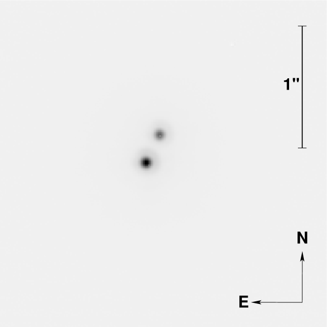
Figure 1: Image of GG Tau A obtained with NACO in October 2009. The separation between the two components is about 250 mas.

The Starfinder program (Diolaiti et al., 2000) was used to measure the positions of the stars. The positions in several images taken during one observation were averaged, and their standard deviation used to estimate the errors. To derive the exact pixel scale and orientation of the detector, we took images of fields in the Orion Trapezium during each observing campaign, and reduced them in the same way as the images of GG Tau. The measured positions of the cluster stars were compared with the coordinates given in McCaughrean & Stauffer (1994). The mean pixel scale and orientation were computed from a global fit of all star positions. The scatter of values derived from star pairs was used to estimate the errors. The errors of the calibration are usually comparable to or larger than the errors of the measured positions of the science target, indicating the importance of a proper astrometric calibration.

The calibrated separations and position angles of GG Tau A appear in Table 1, together with the data taken from the literature. If one or both components of GG Tau B were within the field-of-view, then we also measured their positions. The results appear in Table 2. The main conclusion is that there has been no significant change in the relative position since the first measurement published in Leinert et al. (1993).

Table 1: Astrometric measurements of GG Tau Aa – Ab

Date (UT)	$d$ [mas]		PA $[^{\circ}]$		Reference
1990 Nov 2	$255.$ ${}\pm{}$	$10.$	$9.\phantom{0}$${}\pm{}$	$2.$	Leinert et al. (1993)
1991 Oct 21	$260.$ ${}\pm{}$	$10.$	$2.\phantom{0}$${}\pm{}$	$1.$	Ghez et al. (1995)
1993 Dec 26	$260.$ ${}\pm{}$	$10.$	$3.\phantom{0}$${}\pm{}$	$2.$	Roddier et al. (1996)
1994 Jan 27	$246.$ ${}\pm{}$	$4.$	$357.8$${}\pm{}$	$0.4$	Woitas et al. (2001)
1994 Jul 25	$250.2$ ${}\pm{}$	$2.6$	$358.8$${}\pm{}$	$0.45$	Ghez et al. (1997)
1994 Sep 24	$258.$ ${}\pm{}$	$4.$	$357.\phantom{0}$${}\pm{}$	$2.$	Ghez et al. (1995)
1994 Oct 18	$242.$ ${}\pm{}$	$3.$	$0.9$${}\pm{}$	$0.5$	Ghez et al. (1995)
1994 Dec 22	$239.$ ${}\pm{}$	$5.$	$357.2$${}\pm{}$	$2.$	Roddier et al. (1996)
1995 Oct 8	$247.$ ${}\pm{}$	$4.$	$356.9$${}\pm{}$	$0.7$	Woitas et al. (2001)
1996 Sep 29	$245.$ ${}\pm{}$	$4.$	$355.5$${}\pm{}$	$0.4$	Woitas et al. (2001)
1996 Dec 6	$243.6$ ${}\pm{}$	$4.6$	$354.9$${}\pm{}$	$1.3$	White & Ghez (2001)
1997 Sep 27	$250.$ ${}\pm{}$	$3.$	$354.3$${}\pm{}$	$1.$	Krist et al. (2002)
1997 Oct 10	$248.$ ${}\pm{}$	$2.$	$353.9$${}\pm{}$	$0.4$	McCabe et al. (2002)
1997 Nov 16	$247.$ ${}\pm{}$	$5.$	$353.6$${}\pm{}$	$0.4$	Woitas et al. (2001)
1998 Oct 10	$260.$ ${}\pm{}$	$4.$	$350.7$${}\pm{}$	$0.4$	Woitas et al. (2001)
2001 Jan 21	$248.$ ${}\pm{}$	$14.$	$348.6$${}\pm{}$	$2.4$	Hartigan & Kenyon (2003)
2001 Feb 9	$245.$ ${}\pm{}$	$4.$	$348.7$${}\pm{}$	$0.3$	Tamazian et al. (2002)
2002 Dec 12	$250.7$ ${}\pm{}$	$1.5$	$346.0$${}\pm{}$	$1.5$	Duchêne et al. (2004)
2003 Dec 13	$250.7$ ${}\pm{}$	$0.8$	$344.2$${}\pm{}$	$0.1$	this work
2006 Nov 20	$252.3$ ${}\pm{}$	$0.7$	$339.0$${}\pm{}$	$0.1$	this work
2009 Oct 5	$252.5$ ${}\pm{}$	$0.3$	$334.5$${}\pm{}$	$0.1$	this work

Table 2: Astrometric measurements of GG Tau B

Date (UT)	Pair	$d$ [arcsec]		PA $[^{\circ}]$
2006 Nov 20	Bb–Ba	$1.460$${}\pm{}$	$0.002$	$134.9$${}\pm{}$	$0.1$
	Aa–Ba	$10.07$${}\pm{}$	$0.01$	$185.4$${}\pm{}$	$0.1$
2009 Oct 5	Aa–Ba	$10.09$${}\pm{}$	$0.01$	$185.5$${}\pm{}$	$0.1$

3 Determination of orbital elements

McCabe et al. (2002) and Beust & Dutrey (2005) have determined the orbital elements of GG Tau Aa-Ab from the average position and velocity of the companion. Together with the system mass (Guilloteau et al., 1999), position and velocity on the sky comprise five measurements. Since orbital elements are seven unknowns, their computation requires the additional assumption that the orbit and the circumbinary disk are coplanar.

In this work, we employed a different approach. We fit orbit models to the observations and searched for the model with the minimum $\chi^{2}$. In the end, we wanted to use a Levenberg-Marquardt algorithm (Press et al., 1992). However, the results of this algorithm depend strongly on the chosen start values. To avoid any bias for a particular orbit, we carried out a preliminary fit that consists of a grid search in eccentricity $e$, period $P$, and time of periastron $T_{0}$. Singular value decomposition was used to solve for the remaining four elements. The result is a grid of $\chi^{2}$ as function of $e$ and $P$. Since we were interested in the semi-major axis $a$ of the orbit, this was converted onto a $a$-$e$-grid by finding the orbit model with the closest $a$ for each grid point. The grid spans a range from 20 to 200 AU in $a$, and from 0 to 0.99 in $e$.

To convert the measured separations into AU, a distance of 140 pc was adopted (Elias, 1978).

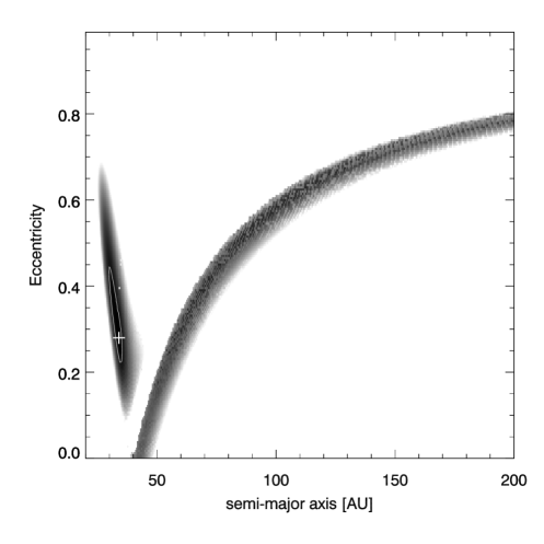
Figure 2: $\chi^{2}$ as function of $a$ and $e$ for orbit models that are coplanar with the circumbinary disk (Sect. 3.1). The cross at $a=34\rm\,AU$, $e=0.28$ marks the minimum, the contour line around it encircles the 99.7 % confidence region (corresponding to $3\sigma$ in the case of normally distributed errors). The areas in various shades of gray are within the $5\sigma$ confidence region, i.e. orbit models in the white area can be excluded with $5\sigma$ confidence.

Figure 3: Best-fitting orbit model if the orbit is constrained to be coplanar with the circumbinary disk (Sect. 3.1). The observed positions are marked by their error ellipses and lines connecting the observed and calculated position at the time of the observations. The new observations with NACO are marked by crosses. Their errors are too small to be discernible. The dash-dotted line indicates the line of nodes, the dashed line the periastron, and the arrow shows the direction of the orbital motion.

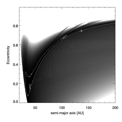
Figure 4: $\chi^{2}$ as function of $a$ and $e$ for orbit models that are not necessarily coplanar with the circumbinary disk (Sect. 3.2). As in Fig. 2, the minimum $\chi^{2}$ is marked by the cross, but the contour line around it encircles the 68.3 % confidence region ($1\sigma$). The areas in shades of gray are within the $5\sigma$ confidence region. The jagged shape of the contour line is most likely caused by numerical effects.

Figure 5: Three exemplary orbit models that fit the astrometric data and the system mass, but are not coplanar with the disk. The semi-major axes of the orbits are 35 AU, 85 AU, and 137 AU. The last orbit has the minimal $\chi^{2}$, and its line of nodes is marked by the dash-dotted line and its periastron by the dashed line. The observed positions are marked by their error ellipses and lines connecting the observed and calculated position at the time of the observations. The new observations with NACO are marked by crosses. Their errors are too small to be discernible.

3.1 Orbits coplanar with the disk

First, we searched for an orbit matching all the information available, i.e. the astrometric position, the total mass, and the orientation of the disk plane. We assumed that disk and orbit are coplanar, orbits without this constraint are discussed in the next section.

The $\chi^{2}$ that we try to minimize is

$$\chi^{2} = \sum_{i}\left(\@vec{r}_{i,\rm obs}-\@vec{r}_{i,\rm model}\over\Delta\@vec{r}_{i,\rm obs}\right)^{2}+\left(M_{\rm est}-M_{\rm model}\over\Delta M_{\rm est}\right)^{2}$$ (1)

$$+\left(i_{\rm disk}-i_{\rm model}\over\Delta i_{\rm disk}\right)^{2}+\left(\Omega_{\rm disk}-\Omega_{\rm model}\over\Delta\Omega_{\rm disk}\right)^{2},$$

where $\@vec{r}_{i,\rm obs}$ and $\@vec{r}_{i,\rm model}$ are the measured and predicted position at the time of observation $i$, and $\Delta\@vec{r}_{i,\rm obs}$ is the error of the measurement. Here, $M_{\rm est}$ is the measured system mass ($1.28\pm 0.07\,M_{\odot}$, Guilloteau et al., 1999), and $M_{\rm model}$ the system mass predicted by the orbit model. Then, $i_{\rm disk}$ and $\Omega_{\rm disk}$ are the inclination and position angle (PA) of the ascending node of the orbit of a disk particle, $\Delta i_{\rm disk}$ and $\Delta\Omega_{\rm disk}$ are their errors. The inclination of the disk is $37\pm 1^{\circ}$ (Guilloteau et al., 1999), but it is in retrograde rotation, so $i_{\rm disk}=180-37=143^{\circ}$. The PA of the minor axis of the disk is $7\pm 2^{\circ}$ (Guilloteau et al., 1999), therefore $\Omega_{\rm disk}=277\pm 2^{\circ}$ (the ascending node is defined as the point in the orbit where the object is receding from the observer most rapidly, e.g. Hilditch, 2001).

Equation 1 was minimized by a Levenberg-Marquardt algorithm (Press et al., 1992). The starting points for the algorithm were taken from the preliminary fit described in the previous section. We kept $a$ and $e$ fixed to preserve the grid in these two variables. The resulting $\chi^{2}$ distribution is depicted in Fig. 2. There is a clear minimum at $a=34\rm\,AU$ and $e=0.28$, while orbits with $a>36\rm\,AU$ can be excluded on the $3\sigma$ level. This is in perfect agreement with previous orbit determinations. The reduced $\chi^{2}$ at the minimum is 3.05, which indicates a less-than-perfect fit. Figure 3 shows the orbit with the minimum $\chi^{2}$, together with the measurements of the relative positions, and Table 3 lists the orbital elements.

Table 3: Parameters of the best orbital solutions.

Orbital Element	Orbit coplanar		Orbit not		most plausible orbit
	with disk		coplanar w. disk		(see Sect. 4)
Date of periastron $T_{0}$	$2477680$	$\,{}^{+690}_{-270}$	$2460050$	$\,{}^{+430}_{-500}$	$2463400$	$\,{}^{+1470}_{-5420}$
	(July 2071)		(April 2023)		(June 2032)
Period $P$ (years)	$162$	$\,{}^{+62}_{-15}$	$1400$	$\,{}^{+17700}_{-1300}$	$403$	$\,{}^{+67}_{-32}$
Semi-major axis $a$ (mas)	$243$	$\,{}^{+38}_{-10}$	$977$	$\,{}^{+96}_{-90}$	$429$
Semi-major axis $a$ (AU)	$34$	$\,{}^{+5.9}_{-2.8}$	$137$	$\,{}^{+17}_{-16}$	$60$
Eccentricity $e$	$0.28$	$\,{}^{+0.05}_{-0.14}$	$0.75$	$\,{}^{+0.03}_{-0.03}$	$0.44$	$\,{}^{+0.02}_{-0.03}$
Argument of periastron $\omega$ (∘)	$91$	$\,{}^{+4}_{-13}$	$8$	$\,{}^{+7}_{-9}$	$19$	$\,{}^{+9}_{-10}$
P.A. of ascending node $\Omega$ (∘)	$277$	$\,{}^{+2.0}_{-2.0}$	$318$	$\,{}^{+10}_{-7}$	$131$	$\,{}^{+13}_{-8}$
Inclination $i$ (∘)	$143$	$\,{}^{+1.3}_{-1.0}$	$128$	$\,{}^{+7}_{-4}$	$132.5$	$\,{}^{+1.0}_{-2.5}$
Angle between orbit and disk	$0.02$	$\,\pm 1.9$	$31.8$	$\,\pm 1.5$	$24.9$	$\,\pm 1.7$

To test whether the astrometric errors were underestimated, we repeated the procedure, but enlarged the errors of the observations by a factor of 3. This lowers $\chi^{2}$ in general, but does not result in significant changes of the shape of the $\chi^{2}$-plane as function of $a$ and $e$. The best-fitting orbit has now $a=40\rm\,AU$ and $e=0.13$. Also, because of the lower $\chi^{2}$, many orbits with $a>36\rm\,AU$ (up to the end of the grid at $a=200\rm\,AU$) are within the 99.7 % confidence region (which corresponds to $3\sigma$ in the case of a normal distribution). However, it appears unlikely that the authors of all astrometric data underestimated their errors by such a large factor, and orbits large enough to cause the disk gap are still only marginally consistent with the data.

3.2 Orbits with no constraint on their orientation

In this section, we remove the constraint that the orbit has to be in the same plane as the circumbinary disk. The only constraints are therefore the astrometric measurements, and the total mass of the binary. Then, $\chi^{2}$ is given by (using the same symbols as in Eq. 1)

$$\chi^{2}=\sum_{i}\left(\@vec{r}_{i,\rm obs}-\@vec{r}_{i,\rm model}\over\Delta\@vec{r}_{i,\rm obs}\right)^{2}+\left(M_{\rm est}-M_{\rm model}\over\Delta M_{\rm est}\right)^{2}.$$ (2)

Figure 4 shows the result of minimizing the $\chi^{2}$ given by Eq. 2. The formal minimum is at $a=137\rm\,AU$, $e=0.75$ (Table 3), with a reduced $\chi^{2}$ of 3.2. It is highly unlikely that the true orbit has such a large semi-major axis and high eccentricity. However, the minimum is very shallow, and no semi-major axis larger than about 30 AU can be excluded, not even at the $1\sigma$ level. Figure 5 shows the orbit with the formally minimal $\chi^{2}$, and two orbits that result in the best fit if the semi-major axis is held fixed at 35 AU and 85 AU, respectively. All three orbits fit the measured data reasonably well, demonstrating that the semi-major axis is not well constrained by the astrometric data.

4 Discussion and conclusions

If we require the orbit model to lie in the same plane as the circumbinary disk, then orbits consistent with the astrometric data are not large enough to explain the gap in the disk. On the other hand, if we consider orbits that are not coplanar with the disk, then the astrometric data only provides a very weak constraint for the semi-major axis. This means that we can easily find orbits that are consistent with the measured positions and with the size of the gap in the circumbinary disk.

According to Artymowicz & Lubow (1994), an orbit with eccentricity $e\approx 0.4\ldots 0.5$ can open a disk gap that is a factor of about 3 larger than its semi-major axis. For our disk with an inner edge at about 180 AU, a semi-major axis of 60 AU would suffice. Figure 5 shows that orbits with $a=60\rm\,AU$ should have an eccentricity of $0.4\ldots 0.45$ to match the astrometric data. We consider this to be the most plausible orbit, given the constraints from the astrometric data and the size of the disk gap. Its orbital elements appear in the rightmost column of Table 3.

Beust & Dutrey (2005) have already discussed noncoplanar solutions for the binary orbit. Assuming $a=62\rm\,AU$ and $e=0.35$, they find $i=125.4^{\circ}$ and four solutions for $\Omega$: $114.3^{\circ}$, $-65.7^{\circ}$, $74.5^{\circ}$, and $-105.6^{\circ}$. The first solution differs from our most plausible orbit by $7^{\circ}$ in inclination and $16.7^{\circ}$ in $\Omega$, which is a reasonable agreement given the large uncertainties.

How large is the misalignment between the plane of the orbit and the plane of the disk? Figure 6 shows the angle between orbit and disk plane as a function of the semi-major axis of the orbit. The relative astrometry of the two stars contains no information about the sign of the inclination (whether the orbit is tilted towards or away from the observer). In the creation of Fig. 6, we adopted in each case the inclination that resulted in the smaller angle between disk and orbit.

Figure 6: Angle between the plane of the binary orbit model and the plane of the circumbinary disk. Plotted are the angles for all orbits within $1\sigma$ of the best fit, i.e. all the orbits within the white contour line in Fig. 4. These are orbit models that were not constrained by the orientation of the disk.

Most orbit models are tilted by less than about 35^∘ with respect to the disk. Our most plausible orbit is inclined by about 25^∘, a significant misalignment. Beust & Dutrey (2005) point out that the disk should show a warped structure if it is not coplanar with the binary orbit. This has not been detected, making such an orbit unlikely, although it cannot be ruled out. Beust & Dutrey (2006) carried out some simulations of the dynamical behavior of the disk for the noncoplanar orbits found by Beust & Dutrey (2005) and a few possible orbits for the outer companion GG Tau B. In all the simulations with the orbit similar to our most plausible orbit (designated AA5 in Beust & Dutrey 2006), the disk tends to assume an open-cone shape with an opening angle of $\sim 30^{\circ}$. This state is reached after 15 million years at the end of simulations. These results suggest that the GG Tau system we observe today is only a transient feature.

GG Tau is only about 1 million years old (White & Ghez, 2001), so it is possible that we happen to observe the disk just before it dissolves into an open cone. We can only speculate how the system got into this unstable state. It is well known that stars experience strong gravitational interactions early in their lifetimes, even if they form in small ensembles of only three to five stars (e.g. Sterzik & Durisen, 1998). These interactions can lead to catastrophic changes in binary orbits and even to the ejection of stars. The four stars in the GG Tau system would be enough to cause such events, unless they are in a stable configuration. Unfortunately, we have no kinematic information about the orbit of GG Tau B, which is not surprising, since we expect an orbital period on the order of 40000 years (based on the projected separation of 1400 AU). It is conceivable that GG Tau has recently suffered a gravitational interaction and is currently in a transient, unstable state. However, a gravitational interaction that changes the orbit of GG Tau A should also have an effect on the circumbinary disk, making it highly unlikely that the disk could maintain the planar structure we see.

On the other hand, the orbital elements derived from the astrometric data have rather large uncertainties. For example, the $1\sigma$ confidence interval for the inclination of the orbit with $a\approx 85\rm\,AU$ ranges from $115^{\circ}$ to $158^{\circ}$ (based on $\chi^{2}$ as function of inclination). The errors of the angle between orbit and disk should be comparable, although not identical, since the angle between orbit and disk also depends on the orientation of the line of nodes.

In summary, we do not have the final answer about the relation between the orbit of GG Tau A and its circumbinary disk. An orbit coplanar with the disk could only cause the inner gap of the disk if the errors of the astrometric measurements are much larger than estimated. An orbit inclined to the plane of the disk would be compatible with both the astrometric data and the disk gap, but it should cause visible distortions in the disk structure. An explanation for the fact that no distortions in the disk have been detected could be that the orbit GG Tau A has only been changed recently, although any effect that can change the orbit of the stars should also disturb the structure of the disk. On the other hand, we should not forget the possibility that the gap in the disk is not related to GG Tau Ab, but some hitherto unknown companion. However, another companion would be pure speculation.

The most likely explanation seems to be a combination of slightly underestimated astrometric errors and a (small) misalignment between the planes of the orbit and the circumbinary disk. More observations over a larger section of the binary orbit are needed.