Magnetic Connectivity between Active Regions 10987, 10988, and 10989 by Means of Nonlinear Force-Free Field Extrapolation

Abstract

Extrapolation codes for modelling the magnetic field in the corona in cartesian geometry do not take the curvature of the Sun’s surface into account and can only be applied to relatively small areas, e.g., a single active region. We apply a method for nonlinear force-free coronal magnetic field modelling of photospheric vector magnetograms in spherical geometry which allows us to study the connectivity between multi-active regions. We use vector magnetograph data from the Synoptic Optical Long-term Investigations of the Sun survey (SOLIS)/Vector Spectromagnetograph(VSM) to model the coronal magnetic field, where we study three neighbouring magnetically connected active regions (ARs: 10987, 10988, 10989) observed on 28, 29, and 30 March 2008, respectively. We compare the magnetic field topologies and the magnetic energy densities and study the connectivities between the active regions(ARs). We have studied the time evolution of magnetic field over the period of three days and found no major changes in topologies as there was no major eruption event. From this study we have concluded that active regions are much more connected magnetically than the electric current.

1 Introduction

S-Introduction In order to model and understand the physical mechanisms underlying the various activity phenomena that can be observed in the solar atmosphere, like, for instance, the onset of flares and coronal mass ejections, the stability of active region, and to monitor the magnetic helicity and free magnetic energy, the magnetic field vector throughout the atmosphere must be known. However, routine measurements of the solar magnetic field are mainly carried out in the photosphere. The magnetic field in the photosphere is measured using the Zeeman effect of magnetically-sensitive solar spectral lines. The problem of measuring the coronal field and its embedded electrical currents thus leads us to use numerical modelling to infer the field strength in the higher layers of the solar atmosphere from the measured photospheric field. Except in eruptions, the magnetic field in the solar corona evolves slowly as it responds to changes in the surface field, implying that the electromagnetic Lorentz forces in this low-$\beta$ environment are relatively weak and that any electrical currents that exist must be essentially parallel or antiparallel to the magnetic field wherever the field is not negligible.

Due to the low value of the plasma $\beta$ (the ratio of gas pressure to magnetic pressure), the solar corona is magnetically dominated [Gary (2001)]. To describe the equilibrium structure of the static coronal magnetic field when non-magnetic forces are negligible, the force-free assumption is appropriate:

$$(\nabla\times\textbf{B})\times\textbf{B}=0\ilabel{one}$$ (1)

$$\nabla\cdot\textbf{B}=0\ilabel{two}$$ (2)

$$\textbf{B}=\textbf{B}_{\textrm{obs}}\quad\mbox{on photosphere}\ilabel{three}$$ (3)

where B is the magnetic field and $\textbf{B}_{\textrm{obs}}$ is measured vector field on the photosphere. Equation (one) states that the Lorentz force vanishes (as a consequence of $\textbf{J}\parallel\textbf{B}$, where J is the electric current density) and Equation (two) describes the absence of magnetic monopoles.

The extrapolation methods based on this assumption are termed nonlinear force-free field extrapolation [Sakurai (1981), Amari et al. (1997), Amari, Boulmezaoud, and Mikic (1999), Amari, Boulmezaoud, and Aly (2006), Wu et al. (1990), Cuperman, Demoulin, and Semel (1991), Demoulin, Cuperman, and Semel (1992), Inhester and Wiegelmann (2006), Mikic and McClymont (1994), Roumeliotis (1996), Yan and Sakurai (2000), Valori, Kliem, and Keppens (2005), Wiegelmann (2004), Wheatland (2004), Wheatland and Régnier (2009), Wheatland and Leka (2010), Amari and Aly (2010)]. For a more complete review of existing methods for computing nonlinear force-free coronal magnetic fields, we refer to the review papers by Amari97, Schrijver06, Metcalf, and Wiegelmann08. Wiegelmann:2006 has developed a code for the self-consistent computation of the coronal magnetic fields and the coronal plasma that uses non-force-free MHD equilibria.

The magnetic field is not force-free in the photosphere, but becomes force-free roughly 400 km above the photosphere [Metcalf et al. (1995)]. Furthermore, measurement errors, in particular for the transverse field components (i.e., perpendicular to the line of sight of the observer), would destroy the compatibility of a magnetogram with the condition of being force-free. One way to ease these problems is to preprocess the magnetogram data as suggested by Wiegelmann06sak. The preprocessing modifies the boundary values of B within the error margins of the measurement in such a way that the moduli of force-free integral constraints of Molodenskii [Molodensky (1974)] are minimized. The resulting boundary values are expected to be more suitable for an extrapolation into a force-free field than the original values.

In the present work, we use a larger computational domain which accommodates most of the connectivity within the coronal region. We also take the uncertainties of measurements in vector magnetograms into account as suggested in DeRosa. We apply a preprocessing procedure to SOLIS data in spherical geometry [Tadesse, Wiegelmann, and Inhester (2009)] by taking account of the curvature of the Sun’s surface. For our observations, performed on 28, 29, and 30 March 2008, respectively, the large field of view contains three active regions (ARs: 10987, 10988, 10989).

The full inversion of SOLIS/VSM magnetograms yields the magnetic filling factor for each pixel, and it also corrects for magneto-optical effects in the spectral line formation. The full inversion is performed in the framework of Milne-Eddington model (ME)[Unno (1956)] only for pixels whose polarization is above a selected threshold. Pixels with polarization below threshold are left undetermined. These data gaps represent a major difficulty for existing magnetic field extrapolation schemes. Due to the large area of missing data in the example treated here in this work, the reconstructed field model obtained must be treated with some caution. It is very likely that the field strength in the area of missing data was small because the inversion procedure, which calculates the surface field from the Stokes line spectra, abandons the calculation if the signal is below a certain threshold. The magnetic field in the corona, however, is dominated by the strongest flux elements on the surface, even if they occupy only a small portion of the surface. We are therefore confident that these dominant flux elements are accounted for in the surface magnetogram, so that the resulting field model is fairly realistic. At any rate, it is the field close to the real, which can be constructed from the available sparse data. Therefore, we use a procedure which allows us to incorporate measurement error and treat regions with lacking observational data as in Tilaye:2010. The technique has been tested in cartesian geometry in Wiegelmann10 for synthetic boundary data.

2 Optimization Principle in Spherical Geometry

Wheatland00 have proposed the variational principle to be solved iteratively which minimizes Lorentz forces (one) and the divergence of magnetic field (two) throughout the volume of interest, $V$. Later on the procedure has been improved by Wiegelmann04 for cartesian geometry in a such way that it can only uses the bottom boundary on the photosphere as an input. Here we use optimization approach for the functional $(\mathcal{L}_{\mathrm{\omega}})$ in spherical geometry [Wiegelmann (2007), Tadesse, Wiegelmann, and Inhester (2009)] and iterate B to minimize $\mathcal{L}_{\mathrm{\omega}}$. The modification concerns the input bottom boundary field $\textbf{B}_{\textrm{obs}}$ which the model field B is not forced to match exactly but we allow deviations of the order of the observational errors. The modified variational problem is [Wiegelmann and Inhester (2010), Tadesse et al. (2011)]:

$$\textbf{B}=\textrm{argmin}(\mathcal{L}_{\omega})$$

$$\mathcal{L}_{\mathrm{\omega}}=\mathcal{L}_{\textrm{f}}+\mathcal{L}_{\textrm{d}}+\nu\mathcal{L}_{\textrm{photo}}\ilabel{four}$$ (4)

$$\mathcal{L}_{\textrm{f}}=\int_{V}\omega_{\textrm{f}}(r,\theta,\phi)B^{-2}\big{|}(\nabla\times\textbf{B})\times\textbf{B}\big{|}^{2}r^{2}\sin\theta drd\theta d\phi$$

$$\mathcal{L}_{\textrm{d}}=\int_{V}\omega_{\textrm{d}}(r,\theta,\phi)\big{|}\nabla\cdot\textbf{B}\big{|}^{2}r^{2}\sin\theta drd\theta d\phi$$

$$\mathcal{L}_{\textrm{photo}}=\int_{S}\big{(}\textbf{B}-\textbf{B}_{\textrm{obs}}\big{)}\cdot\textbf{W}(\theta,\phi)\cdot\big{(}\textbf{B}-\textbf{B}_{\textrm{obs}}\big{)}r^{2}\sin\theta d\theta d\phi$$

where $\mathcal{L}_{\mathrm{\textrm{f}}}$ and $\mathcal{L}_{\mathrm{\textrm{d}}}$ measure how well the force-free Equations (one) and divergence-free (two) conditions are fulfilled, respectively. $\omega_{\textrm{f}}(r,\theta,\phi)$ and $\omega_{\textrm{d}}(r,\theta,\phi)$ are weighting functions for force-free term and divergence-free term, respectively and identical for this study. The third integral, $\mathcal{L}_{\textrm{photo}}$, is a surface integral over the photosphere which serves to relax the field on the photosphere towards a force-free solution without too much deviation from the original surface field data, $\textbf{B}_{\textrm{obs}}$. In this integral, $\textbf{W}(\theta,\phi)=\textrm{diag}(w_{\textrm{radial}},w_{\textrm{trans}},w_{\textrm{trans}})$ is diagonal matrix which gives different weights for observed surface field components depending on its relative accuracy in measurement. In this sense, lacking data is considered most inaccurate and is taken account of by setting $W(\theta,\phi)$ to zero in all elements of the matrix.

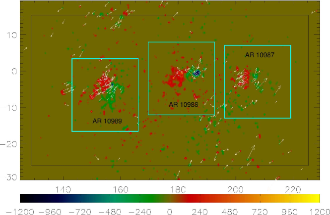
Figure 1.: Surface contour plot of radial magnetic field component and vector field plot of transverse field with white arrows. The color coding shows $B_{r}$ on the photosphere. The vertical and horizontal axes show latitude, $\theta$(in degree) and longitude, $\phi$(in degree) on the photosphere. In the area coloured in olive, field values are lacking. The region inside the black box corresponds to the physical domain where the weighting function is unity and the outside region is the buffer zone where it declines to zero. The blue boxes indicate the domains of the three active regions.fig1

We use a spherical grid $r$, $\theta$, $\phi$ with $n_{r}$, $n_{\theta}$, $n_{\phi}$ grid points in the direction of radius, latitude, and longitude, respectively. In the code, we normalize the magnetic field with the average radial magnetic field on the photosphere and the length scale with a solar radius for numerical reason. Figure fig1 shows a map of the radial component of the field as color-coded and the transverse magnetic field depicted as white arrows. For this particular dataset, about $86\%$ of the data pixels are undetermined. The method works as follows:

• We compute an initial source surface potential field in the computational domain from $\textbf{B}_{\textrm{obs}}\cdot\hat{r}$, the normal component of the surface field at the photosphere at $r=1R_{\mathrm{\odot}}$. The computation is performed by assuming that a currentless ($\textbf{J}=0$ or $\nabla\times\textbf{B}=0$) approximation holds between the photosphere and some spherical surface $S_{s}$ (source surface where the magnetic field vector is assumed radial). We compute the solution of this boundary-value problem in a standard form of spherical harmonics expansion.

• We minimize $\mathcal{L}_{\omega}$(Equations four) iteratively. The model magnetic field B at the surface is gradually driven towards the observed field $\textbf{B}_{\textrm{obs}}$ while the field in the volume $V$ relaxes to force-free. If the observed field, $\textbf{B}_{\textrm{obs}}$, is inconsistent, the difference $\textbf{B}-\textbf{B}_{\textrm{obs}}$ remains finite depending in the control parameter $\nu$. At data gaps in $\textbf{B}_{\textrm{obs}}$, the respective field value is automatically ignored.

• The iteration stops when $\mathcal{L}_{\omega}$ becomes stationary as $\Delta\mathcal{L}_{\omega}/\mathcal{L}_{\omega}<10^{-4}$, $\Delta\mathcal{L}_{\omega}$ is the decrease of $\mathcal{L}_{\omega}$ during an iterative steps.

• A convergence to $\mathcal{L}_{\omega}=0$ yields a perfect force-free and divergence-free state and exact agreement of the boundary values B with observations $\textbf{B}_{\textrm{obs}}$ in regions where the elements of W are greater than zero. For inconsistent boundary data the force-free and solenoidal conditions can still be fulfilled, but the surface term $\mathcal{L}_{\textrm{photo}}$ will remain finite. This results in some deviation of the bottom boundary data from the observations, especially in regions where $w_{\textrm{radial}}$ and $w_{\textrm{trans}}$ are small. The parameter $\nu$ is tuned so that these deviations do not exceed the local estimated measurement error.

3 Results

In this work, we apply our extrapolation scheme to Milne-Eddington inverted vector magnetograph data from the Synoptic Optical Long-term Investigations of the Sun survey (SOLIS). As a first step for our work we remove non-magnetic forces from the observed surface magnetic field using our spherical preprocessing procedure. The code takes $\textbf{B}_{\textrm{obs}}$ as improved boundary condition.

SOLIS/VSM provides full-disk vector-magnetograms, but for some individual pixels the inversion from line profiles to field values may not have been successful inverted and field data there will be missing for these pixels (see Figure fig1). The different errors for the radial and transverse components of $\textbf{B}_{\textrm{obs}}$ are taken account by different values for $w_{\textrm{radial}}$ and $w_{\textrm{trans}}$. In this work we used $w_{\textrm{radial}}=20w_{\textrm{trans}}$ for the surface preprocessed fields as the radial component of $\textbf{B}_{\textrm{obs}}$ is measured with higher accuracy.

We compute the 3D magnetic field above the observed surface region inside wedge-shaped computational box of volume $V$, which includes an inner physical domain $V^{\prime}$ and a buffer zone(the region outside the physical domain), as shown in Figure fig1b. The physical domain $V^{\prime}$ is a wedge-shaped volume, with two latitudinal boundaries at $\theta_{\textrm{min}}=-26^{\circ}$ and $\theta_{\textrm{max}}=16^{\circ}$, two longitudinal boundaries at $\phi_{\textrm{min}}=129^{\circ}$ and $\phi_{\textrm{max}}=226^{\circ}$, and two radial boundaries at the photosphere ($r=1R_{\odot}$) and $r=1.75R_{\odot}$. Note that the longitude $\phi$ is measured from the center meridian of the back side of the disk.

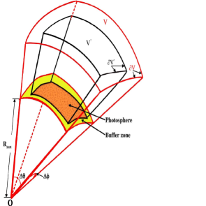
Figure 2.: Wedge-shaped computational box of volume $V$ with the inner physical domain $V^{\prime}$ and a buffer zone. O is the center of the Sun.fig1b

        

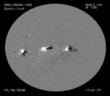
(a) 28 March 2008 15:45UT

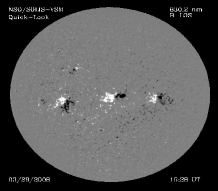
(b) 29 March 2008 15:48UT

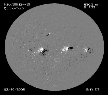
(c) 30 March 2008 15:47UT

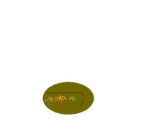
(d) 28 March 2008 15:45UT

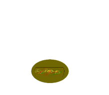
(e) 29 March 2008 15:48UT

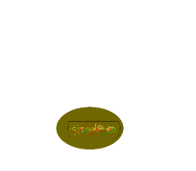
(f) 30 March 2008 15:47UT

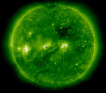
(g) 28 March 2008 16:00UT

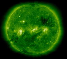
(h) 29 March 2008 15:48UT

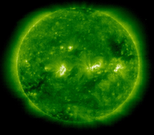
(i) 30 March 2008 15:48UT

Figure 3.: Top row: SOLIS/VSM magnetograms of respective dates. Middle row: Magnetic field lines reconstructed from magnetograms on the top panel. Bottom row: EIT image of the Sun at 195Å on indicated dates. fig2

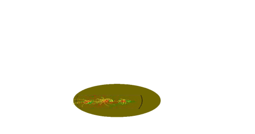
(a) 28 March 2008 15:45UT

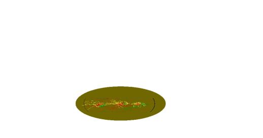
(b) 29 March 2008 15:48UT

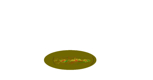
(c) 30 March 2008 15:47UT

Figure 4.: Some magnetic field lines plots reconstructed from SOLIS magnetograms using nonlinear force-free modelling. The color coding shows $B_{r}$ on the photosphere.fig3

We define $V^{\prime}$ to be the inner region of $V$ (including the photospheric boundary) with $\omega_{\textrm{f}}=\omega_{\textrm{d}}=1$ everywhere including its six inner boundaries $\delta V^{\prime}$. We use a position-dependent weighting function to introduce a buffer boundary of $nd=10$ grid points towards the side and top boundaries of the computational box, $V$. The weighting functions, $\omega_{\textrm{f}}$ and $\omega_{\textrm{d}}$ are chosen to be unity within the inner physical domain $V^{\prime}$ and decline to 0 with a cosine profile in the buffer boundary region [Wiegelmann (2004), Tadesse, Wiegelmann, and Inhester (2009)]. The framed region in Figure fig1 corresponds to the lower boundary of the physical domain $V^{\prime}$ with a resolution of $114\times 251$ pixels in the photosphere.

The middle panel of Figure fig2 shows magnetic field line plots for three consecutive dates of observation. The top and bottom panels of Figure fig2 show the position of the three active regions on the solar disk both for SOLIS full-disk magnetogram and SOHO/EIT image of the Sun observed at 195Å on the indicated dates and times. Figure fig3 shows some selected magnetic field lines from reconstruction from the SOLIS magnetograms, zoomed in from the middle panels of Figure fig2. In each column of Figure fig3 the field lines are plotted from the same foot points to compare the change in topology of the magnetic field over the period of the three days of observation. In order to compare the fields at the three consecutive days quantitatively, we computed the vector correlations between the three field configurations. The vector correlation ($C_{\mathrm{\textrm{vec}}}$) [Schrijver et al. (2006)] metric generalizes the standard correlation coefficient for scalar functions and is given by

$$C_{\mathrm{\textrm{vec}}}=\frac{\sum_{i}\textbf{v}_{i}\cdot\textbf{u}_{i}}{\sqrt{\sum_{i}|\textbf{v}_{i}|^{2}}\sqrt{\sum_{i}|\textbf{u}_{i}|^{2}}}\ilabel{nine}$$ (5)

where $\textbf{v}_{i}$ and $\textbf{u}_{i}$ are 3D vectors at grid point $i$. If the vector fields are identical, then $C_{\textrm{vec}}=1$; if $\textbf{v}_{i}\perp\textbf{u}_{i}$ , then $C_{\textrm{vec}}=0$. The correlations ($C_{\mathrm{\textrm{vec}}}$) of the 3D magnetic field vectors of 28 and 30 March with respect to the field on 29 March are $0.96$ and $0.93$ respectively. From these values we can see that there has been no major change in the magnetic field configuration during this period.

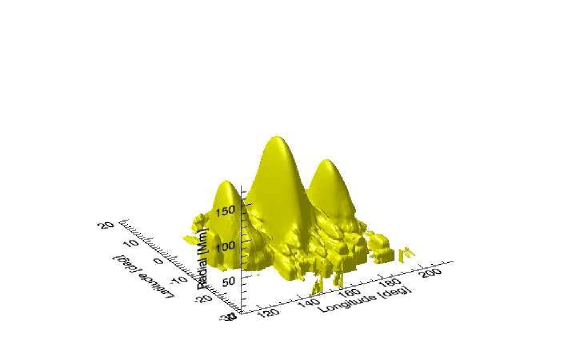
(a) 28 March 2008 15:45UT

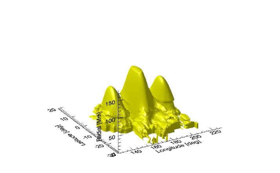
(b) 29 March 2008 15:48UT

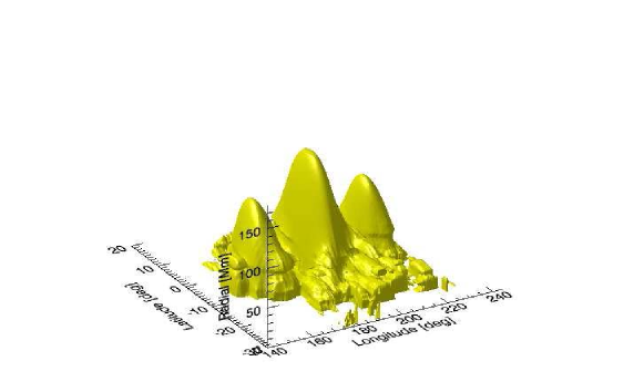
(c) 30 March 2008 15:47UT

Figure 5.: Iso-surfaces (ISs) of the absolute NLFF magnetic energy density ($7.5\times 10^{16}$erg) for the three consecutive dates computed within the entire computational domain.fig4

We also compute the values of the free magnetic energy estimated from the excess energy of the extrapolated field beyond the potential field satisfying the same $\textbf{B}_{\textrm{obs}}\cdot\hat{r}$ boundary condition. Similar estimates have been made by Regnier and Thalmann for single active regions observed at other times. From the corresponding potential and force-free magnetic field, $\textbf{B}_{\textrm{pot}}$ and B, respectively, we can estimate an upper limit to the free magnetic energy associated with coronal currents

$$E_{\mathrm{free}}=E_{\mathrm{\textrm{nlff}}}-E_{\mathrm{\textrm{pot}}}=\frac{1}{8\pi}\int_{V^{\prime}}\Big{(}B_{\textrm{nlff}}^{2}-B_{\textrm{pot}}^{2}\Big{)}r^{2}\textrm{sin}\theta drd\theta d\phi.\ilabel{ten}$$ (6)

Date	$E_{\textrm{nlff}}(10^{32}\textrm{erg})$	$E_{\mathrm{\textrm{pot}}}(10^{32}\textrm{erg})$	$E_{\mathrm{free}}(10^{32}\textrm{erg})$
28 March 2008	$57.34$	$53.89$	$3.45$
29 March 2008	$57.48$	$54.07$	$3.41$
30 March 2008	$57.37$	$53.93$	$3.44$

Table 1.: The magnetic energy associated with extrapolated NLFF field configurations for the three particular dates.table1

The computed energy values are listed in Table table1. The free energy on all three days is about $3.5\times 10^{32}\textrm{erg}$. The magnetic energy associated with the potential field configuration is about $54\times 10^{32}\textrm{erg}$. Hence $E_{\textrm{nlff}}$ exceeds $E_{\textrm{pot}}$ by only 6$\%$. Figure fig4 shows Iso-surface plots of magnetic energy density in the volume above the active regions. There are strong energy concentrations above each active region. There were no major changes in the magnetic energy density over the observation period and there was no major eruptive phenomenon during those three days in the region observed.

In our previous work[Tadesse et al. (2011)], we have studied the connectivity between two neighbouring active regions. In this work with an even larger field of view, the three ARs share a decent amount of magnetic flux compared to their internal flux from one polarity to the other (see Figure fig3). In terms of the electric current they are much more isolated. In order to quantify these connectivities, we have calculated the magnetic flux and the electric currents shared between active regions. For the magnetic flux, e.g., we use

$$\Phi_{\alpha\beta}=\sum_{i}|\textbf{B}_{i}\cdot\hat{r}|R^{2}_{\odot}\textrm{sin}(\theta_{i})\Delta\theta_{i}\Delta\phi_{i}\ilabel{ten}$$ (7)

where the summation is over all pixels of $\mbox{AR}_{\alpha}$ from which the field line ends in $\mbox{AR}_{\beta}$ or $i\in\mbox{AR}_{\alpha}\|\,\mbox{conjugate footpoint}(i)\in\mbox{AR}_{\beta}$. The indices $\alpha$ and $\beta$ denote the active regions and the index number $1$ corresponds to AR $10989$, $2$ to AR $10988$ and $3$ to AR $10987$ of Figure fig1. For the electric current we replace the magnetic field, $\textbf{B}_{i}\cdot\hat{r}$, by the vertical current density $\textbf{J}_{i}\cdot\hat{r}$ in Equation (ten). Whenever the end point of a field line falls outside (blue rectangles in Figure fig1) of the three ARs, we categorize it as ending elsewhere. Both Table table2 and table3 show the percentage of the total magnetic flux and electric current shared between the three ARs. So, for example first column of Table table2 shows that $56.37\%$ of positive polarity of $\mbox{AR}_{1}$ is connected to negative polarity of $\mbox{AR}_{1}$; line 2 shows that $13.66\%$ of positive/negative polarity of $\mbox{AR}_{1}$ is connected to positive/negative polarity of $\mbox{AR}_{2}$, and line 3 shows that there are no field lines $(0\%)$ connecting positive/negative polarity of $\mbox{AR}_{1}$ with positive/negative polarity of $\mbox{AR}_{3}$. The same technique applies for Table table3 too. The three active regions are magnetically connected but much less by electric currents.

		$28th$			$29th$			$30th$
$\Phi_{\alpha\beta}$	$\alpha=1$	$2$	$3$	$\alpha=1$	$2$	$3$	$\alpha=1$	$2$	$3$
$\beta=1$	$56.37$	$5.59$	$0.00$	$56.50$	$5.48$	$0.00$	$56.50$	$5.48$	$0.00$
$2$	$13.66$	$81.12$	$1.43$	$13.66$	$81.22$	$1.43$	$13.66$	$81.22$	$2.22$
$3$	$0.00$	$0.48$	$71.47$	$0.00$	$0.48$	$71.80$	$0.00$	$0.48$	$71.80$
Elsewhere	$29.97$	$12.82$	$27.10$	$29.84$	$12.82$	$26.77$	$29.84$	$12.82$	$25.98$

Table 2.: The percentage of the total magnetic flux shared between the three ARs. $\Phi_{11}$, $\Phi_{22}$ and $\Phi_{33}$ denote magnetic flux of AR 10989(left), AR 10988(middle) and AR 10987(right) of Figure fig1, respectively. table2

		$28th$			$29th$			$30th$
$I_{\alpha\beta}$	$\alpha=1$	$2$	$3$	$\alpha=1$	$2$	$3$	$\alpha=1$	$2$	$3$
$\beta=1$	$82.47$	$0.19$	$0.00$	$86.36$	$0.19$	$0.00$	$94.16$	$0.19$	$0.00$
$2$	$0.65$	$85.25$	$1.42$	$0.65$	$85.25$	$1.42$	$0.65$	$85.25$	$3.55$
$3$	$0.00$	$0.38$	$82.27$	$0.00$	$0.38$	$82.27$	$0.00$	$0.38$	$82.27$
Elsewhere	$16.88$	$14.18$	$16.31$	$12.99$	$14.18$	$16.31$	$5.19$	$14.18$	$14.18$

Table 3.: The percentage of the total electric current shared between the three ARs. $I_{11}$, $I_{22}$, and $I_{33}$ denote electric current of AR 10989(left), AR 10988(middle) and AR 10987(right) of Figure fig1, respectively. table3

4 Conclusions

sect:disc We have investigated the coronal magnetic field associated with three ARs 10987, 10987, 10989, on 28, 29 and 30 March 2008 by analysing SOLIS/VSM data. We have used an optimization method for the reconstruction of nonlinear force-free coronal magnetic fields in spherical geometry by restricting the code to limited parts of the Sun [Wiegelmann (2007), Tadesse, Wiegelmann, and Inhester (2009), Tadesse et al. (2011)]. The code was modified so that it allows us to deal with lacking data and regions with poor signal-to-noise ratio in a systematic manner[Wiegelmann and Inhester (2010), Tadesse et al. (2011)].

We have studied the time evolution of magnetic field over the period of three days and found no major changes in topologies as there was no major eruption event. The magnetic energies calculated in the large wedge-shaped computational box above the three active regions were not far apart in value. This is the first study which contains three well separated ARs in our model. This was made possible by the use of spherical coordinates and it allows us to analyse linkage between the ARs. The active regions share a decent amount of magnetic flux compared to their internal flux from one polarity to the other. In terms of the electric current they are much more isolated.

References

- Amari and Aly (2010) Amari, T., Aly, J.: 2010,. Astron. Astrophys. 522, A52.
- Amari, Boulmezaoud, and Aly (2006) Amari, T., Boulmezaoud, T.Z., Aly, J.J.: 2006,. Astron. Astrophys. 446, 691.
- Amari, Boulmezaoud, and Mikic (1999) Amari, T., Boulmezaoud, T.Z., Mikic, Z.: 1999,. Astron. Astrophys. 350, 1051.
- Amari et al. (1997) Amari, T., Aly, J.J., Luciani, J.F., Boulmezaoud, T.Z., Mikic, Z.: 1997,. Solar Phys. 174, 129.
- Cuperman, Demoulin, and Semel (1991) Cuperman, S., Demoulin, P., Semel, M.: 1991,. Astron. Astrophys. 245, 285.
- Demoulin, Cuperman, and Semel (1992) Demoulin, P., Cuperman, S., Semel, M.: 1992,. Astron. Astrophys. 263, 351.
- DeRosa et al. (2009) DeRosa, M.L., Schrijver, C.J., Barnes, G., Leka, K.D., Lites, B.W., Aschwanden, M.J., et al.: 2009,. Astrophys. J. 696, 1780.
- Gary (2001) Gary, G.A.: 2001,. Solar Phys. 203, 71.
- Inhester and Wiegelmann (2006) Inhester, B., Wiegelmann, T.: 2006,. Solar Phys. 235, 201.
- Metcalf et al. (1995) Metcalf, T.R., Jiao, L., McClymont, A.N., Canfield, R.C., Uitenbroek, H.: 1995,. Astrophys. J. 439, 474.
- Metcalf et al. (2008) Metcalf, T.R., Derosa, M.L., Schrijver, C.J., Barnes, G., van Ballegooijen, A.A., Wiegelmann, T., Wheatland, M.S., Valori, G., McTtiernan, J.M.: 2008,. Solar Phys. 247, 269.
- Mikic and McClymont (1994) Mikic, Z., McClymont, A.N.: 1994,, Astronomical Society of the Pacific Conference Series 68, 225.
- Molodensky (1974) Molodensky, M.M.: 1974,. Solar Phys. 39, 393.
- Régnier and Priest (2007) Régnier, S., Priest, E.R.: 2007,. Astrophys. J. Lett. 669, L53.
- Roumeliotis (1996) Roumeliotis, G.: 1996,. Astrophys. J. 473, 1095.
- Sakurai (1981) Sakurai, T.: 1981,. Solar Phys. 69, 343.
- Schrijver et al. (2006) Schrijver, C.J., Derosa, M.L., Metcalf, T.R., Liu, Y., McTiernan, J., Régnier, S., Valori, G., Wheatland, M.S., Wiegelmann, T.: 2006,. Solar Phys. 235, 161.
- Tadesse, Wiegelmann, and Inhester (2009) Tadesse, T., Wiegelmann, T., Inhester, B.: 2009,. Astron. Astrophys. 508, 421.
- Tadesse et al. (2011) Tadesse, T., Wiegelmann, T., Inhester, B., Pevtsov, A.: 2011,. Astron. Astrophys. 527, A30.
- Thalmann, Wiegelmann, and Raouafi (2008) Thalmann, J.K., Wiegelmann, T., Raouafi, N.E.: 2008,. Astron. Astrophys. 488, L71.
- Unno (1956) Unno, W.: 1956,. Publ. Astron. Soc. Japan 8, 108.
- Valori, Kliem, and Keppens (2005) Valori, G., Kliem, B., Keppens, R.: 2005,. Astron. Astrophys. 433, 335.
- Wheatland (2004) Wheatland, M.S.: 2004,. Solar Phys. 222, 247.
- Wheatland and Leka (2010) Wheatland, M.S., Leka, K.D.: 2010,. ArXiv e-prints.
- Wheatland and Régnier (2009) Wheatland, M.S., Régnier, S.: 2009,. Astrophys. J. Lett. 700, L88.
- Wheatland, Sturrock, and Roumeliotis (2000) Wheatland, M.S., Sturrock, P.A., Roumeliotis, G.: 2000,. Astrophys. J. 540, 1150.
- Wiegelmann (2004) Wiegelmann, T.: 2004,. Solar Phys. 219, 87.
- Wiegelmann (2007) Wiegelmann, T.: 2007,. Solar Phys. 240, 227.
- Wiegelmann (2008) Wiegelmann, T.: 2008,. J. Geophys. Res. 113, 3.
- Wiegelmann and Inhester (2010) Wiegelmann, T., Inhester, B.: 2010,. Astron. Astrophys. 516, A107.
- Wiegelmann and Neukirch (2006) Wiegelmann, T., Neukirch, T.: 2006,. Astron. Astrophys. 457, 1053.
- Wiegelmann, Inhester, and Sakurai (2006) Wiegelmann, T., Inhester, B., Sakurai, T.: 2006,. Solar Phys. 233, 215.
- Wu et al. (1990) Wu, S.T., Sun, M.T., Chang, H.M., Hagyard, M.J., Gary, G.A.: 1990,. Astrophys. J. 362, 698.
- Yan and Sakurai (2000) Yan, Y., Sakurai, T.: 2000,. Solar Phys. 195, 89.