Unveiling the 3D temperature structure of galaxy clusters by means of the thermal Sunyaev-Zel’dovich effect

Abstract

The Sunyaev-Zel’dovich (hereafter SZ) effect is a promising tool to derive the gas temperature of galaxy clusters. The approximation of a spherically symmetric gas distribution is usually used to determine the temperature structure of galaxy clusters, but this approximation cannot properly describe merging galaxy clusters. The methods used so far, which do not assume the spherically symmetric distribution, permit us to derive 2D temperature maps of merging galaxy clusters. In this paper, we propose a method to derive the standard temperature deviation and temperature variance along the line-of-sight, which permits us to analyze the 3D temperature structure of galaxy clusters by means of the thermal SZ effect. We also propose a method to reveal merger shock waves in galaxy clusters by analyzing the presence of temperature inhomogeneities along the line-of-sight.

1 Introduction

Galaxy clusters are large gravitationally bound structures of a size of $\sim$1–3 Mpc, which have arisen in the hierarchical structure formation of the Universe. Intergalactic gas fills the space between galaxies in the clusters. The typical number density and temperature values of this intergalactic gas are $10^{-1}$–$10^{-3}$ cm^-3 and 2-10 keV, respectively(for a review, see e.g., Sarazin 1986). Inverse Compton scattering between cosmic microwave background (CMB) photons and hot free electrons in clusters of galaxies causes a change in the intensity of the CMB radiation towards clusters of galaxies (the Sunyaev-Zel’dovich effect, hereinafter the SZ effect; for a review, see Sunyaev & Zel’dovich 1980).

The SZ effect is an important tool for the study of clusters of galaxies (for a review, see Birkinshaw 1999), since both the amplitude and spectral form of the CMB distortion caused by the SZ effect depend on the intergalactic gas parameters (such as the gas number density and temperature). A relativistically correct formalism for the SZ effect based on the probability distribution of the photon frequency shift after scattering was given by Wright (1979) to describe the Comptonization process of soft photons by high temperature plasma. SZ relativistic corrections are significant even for galaxy clusters with temperatures of 3-5 keV and allow us to derive the gas temperature from SZ observations (see, e.g., Colafrancesco & Marchegiani 2010). The constraints on the gas temperature of high temperature clusters from measurements of SZ relativistic corrections have been firstly obtained by Pointecouteau et al. (1998) and Hansen et al. (2002). The imaging and spectroscopic capabilities of coming SZ experiments will permit us to analyze the gas temperature structure even in relatively cool galaxy clusters (Colafrancesco & Marchegiani 2010).

Using hydrodynamic simulations of galaxy clusters, Kay et al. (2008) compared the temperatures derived from the X-ray spectroscopy (the X-ray temperature) and from the SZ effect (the SZ temperature). They demonstrated that the SZ temperature corresponds to the Compton-averaged electron temperature for relatively cool galaxy clusters. Their SZ temperature map is directly calculated from the simulated temperature and density distributions.

Colafrancesco & Marchegiani (2010) show how to obtain detailed information about the cluster temperature distribution for spherically–symmetric galaxy clusters. However, the approximation of a spherical symmetry cannot properly describe merging galaxy clusters. Signatures of shock waves caused by galaxy cluster mergers are imprinted on the 2D X-ray surface brightness maps of merging galaxy clusters (for a review, see Markevitch & Vikhlinin 2007) and, therefore, merger shocks should be included in a realistic modeling of the SZ effect from merging galaxy clusters. Prokhorov et al. (2010b) incorporated the relativistic Wright formalism for modeling the SZ effect from a merging galaxy cluster in a numerical simulation and introduced a method to derive the SZ temperature that does not require symmetry and so is suitable for merging clusters.

In this paper, we extend the previous studies by introducing a method to derive the standard temperature deviation and temperature variance along the line-of-sight for revealing the 3D temperature structure for relatively cool merging galaxy clusters with temperatures less than 10 keV. We focus on relatively cool merging galaxy clusters because it is easier to measure their standard temperature deviation and temperature variance owing to lower order SZ corrections.

Shock-heated regions have been found by Chandra in numerous galaxy clusters in the range from galaxy groups with temperatures of $\approx$ 1 keV, such a HGC 62 (Gitti et al. 2010), to the most massive galaxy clusters with temperatures of $\approx$ 15 keV, such as the Bullet cluster (Markevitch et al. 2002). In this paper, we show that the temperature variance along the line-of-sight is an useful quantity, which allows us to reveal shocks in galaxy clusters, and demonstrate how to reveal a merger shock by analyzing a relatively cool simulated galaxy cluster.

We also propose an extension of our method to make it suitable for hot galaxy clusters (in the temperature range of 10 keV – 15 keV). We calculate the temperature variance along the line-of-sight for a simulated hot galaxy cluster to demonstrate how this quantity can be derived from multi-frequency observations of the SZ effect.

Studying the presence of gas inhomogeneities along the line-of-sight by means of the SZ effect is important to improve our knowledge of the 3D temperature structure of merging galaxy clusters. This will permit us to improve the deprojection analysis of galaxy clusters by comparing the derived values of the standard temperature deviation along the line-of-sight with those calculated from the deprojection maps. An analysis of maps of the gas temperature variance along the line-of-sight will provide us with an interesting approach to reveal merger shocks. This approach is alternative to that based on the projected X-ray surface brightness maps (e.g. Markevitch et al. 2002).

The layout of the paper is as follows. We calculate the SZ intensity maps of the simulated galaxy cluster at frequencies of 150 GHz and 217 GHz in the framework of the Wright formalism in Sect. 2. We propose a method to derive the temperature variance along the line-of-sight for relatively cool galaxy clusters and apply this method to the simulated galaxy cluster in Sect. 3, using the derived SZ intensity maps. We also propose a method to reveal merger shocks in the simulated galaxy cluster in Sect. 3. We present our discussion on how to improve the proposed method and calculate the temperature variance for a simulated hot galaxy cluster in Sects. 4 and 5, respectively. We present our conclusions in Sect. 6.

2 The SZ effect from the simulated cluster

In this section, we calculate the SZ intensity maps at frequencies of 150 GHz and 217 GHz in the framework of the relativistic Wright formalism for the merging galaxy cluster simulated by Dubois et al. (2010) and previously analyzed by means of the SZ effect by Prokhorov et al. (2010b). The derived SZ intensity maps will be used in the next section to calculate the temperature variance along the line-of-sight.

The galaxy cluster simulations of Dubois et al. (2010), which we use in this paper, are run with the Adaptive Mesh Refinement (AMR) code RAMSES (Teyssier 2002). The simulation follows the gas dynamics using a second-order unsplit Godunov scheme for the Euler equations with a Total Variation Diminishing scheme for extrapolation of fluid quantities at the cell interface from their cell centre values. Particles are evolved with a particle-mesh solver for gravity and using a Cloud-In-Cell interpolation.

The simulation includes gas cooling from a primordial gas composition of Hydrogen and Helium with a UV heating background following Haardt & Madau (1996). The reionization redshift is set up at $z=8.5$. Star formation proceeds in high gas-density regions with $\rho>0.1\,\rm H\,\rm cm^{-3}$ (Rasera & Teyssier 2006, Dubois & Teyssier 2008). Though feedback from supernovae is not included, we take into account the feedback from Active Galactic Nuclei following the model from Dubois et al. (2010), which is the dominant source of energy in massive objects such as galaxy clusters.

The simulation is performed assuming a flat $\Lambda$CDM cosmology (Spergel et al. 2003). A zoom technique is employed with a $128^{3}$ coarse grid in a 80 $h^{-1}_{100}$ Mpc box size, and with two nested grids with a 20 $h^{-1}_{100}$ Mpc and a 6 $h^{-1}_{100}$ Mpc radius for a $256^{3}$ and $512^{3}$ equivalent grid respectively, where $h_{100}=H_{0}/(100\,\rm km\,\rm s^{-1}\,\rm Mpc^{-1})$. This leads to a minimum dark matter mass of $M_{\rm DM}=4.5\times 10^{8}\,\rm M_{\odot}$. The grid is dynamically refined down to level $16$, reaching 1.19 $h^{-1}_{100}$ kpc. The zoom region tracks the formation of a galaxy cluster with a 1:1 major merger occurring at z = 0.8. This z = 0.8 major galaxy merger drives the cluster gas to temperatures twice the virial temperature thanks to violent shock waves. The projected mass-weighted temperature map is shown in Fig. 2. For further details of the simulation, see Dubois et al. (2010).

Using the Wright formalism, we have previously calculated the SZ intensity maps at frequencies of 128 GHz and 369 GHz for the simulated cluster at z=0.74 (see Prokhorov et al. 2010b). These frequencies correspond to minimum and maximum values of the SZ intensity in the the Kompaneets approximation (Kompaneets 1957). The ratio of these SZ intensities has allowed us to derive the SZ-temperature from mock SZ observations. The derived SZ-temperature is shown in Fig. 2 (top left-hand panel) and demonstrates how the prominent structures on the 2D projected temperature map of the merging cluster can be unveiled. The mass-weighted temperature map (in keV) of the simulated cluster is plotted in Fig. 2 (top right-hand panel) for a comparison. The gas temperature maps have prominent “arc-like” structures, which have a high temperature compared with other simulated cluster regions. The average temperature of the “arc-like” structures is $\approx$5 keV and, therefore, we can use this simulated cluster as an example of a relatively low temperature galaxy cluster. Below, we briefly describe how to calculate the SZ intensity maps in the framework of the Kompaneets and Wright formalisms.

The CMB intensity distortion caused by the SZ effect on a non-relativistic electron population in the framework of the Kompaneets approximation is given by (for a review, see Birkinshaw 1999)

$$\Delta I_{\mathrm{nr}}(x)=I_{\mathrm{0}}g(x)y_{\mathrm{gas}},$$ (1)

where $I_{\mathrm{0}}=2(k_{\mathrm{b}}T_{\mathrm{cmb}})^{3}/(hc)^{2}$, $x=h\nu/k_{\mathrm{b}}T_{\mathrm{cmb}}$, and the spectral shape of the SZ distortion is described by the spectral function

$$g(x)=\frac{x^{4}\exp(x)}{(\exp(x)-1)^{2}}\left(x\frac{\exp(x)+1}{\exp(x)-1}-4\right).$$ (2)

The subscript $`\mathrm{nr}^{\prime}$ denotes that Eq. (1) was obtained for a non-relativistic electron population in the Kompaneets approximation. The Comptonization parameter $y_{\mathrm{gas}}$ is given by

$$y_{\mathrm{gas}}=\frac{\sigma_{\mathrm{T}}}{m_{\mathrm{e}}c^{2}}\int n_{\mathrm{gas}}kT_{\mathrm{e}}dl,$$ (3)

where the integral must be taken along the line-of-sight, $T_{\mathrm{e}}$ is the electron temperature, $n_{\mathrm{gas}}$ is the number density of the gas, $\sigma_{\mathrm{T}}$ is the Thomson cross-section, $m_{\mathrm{e}}$ the electron mass, $c$ the speed of light, $k_{\mathrm{b}}$ the Boltzmann constant, and $h$ the Planck constant.

The CMB intensity distortion caused by the SZ effect in the relativistic Wright formalism can be written in the form proposed by Prokhorov et al. (2010a) given by

$$\Delta I(x)=I_{\mathrm{0}}\frac{\sigma_{\mathrm{T}}}{m_{\mathrm{e}}c^{2}}\int n_{\mathrm{gas}}k_{\mathrm{b}}T_{\mathrm{e}}G(x,T_{\mathrm{e}})dl,$$ (4)

where $G(x,T_{\mathrm{e}})$ is the generalized spectral function, which depends explicitly on the electron temperature.

The relativistic spectral function $G(x,T_{\mathrm{e}})$ obtained in the framework of the Wright formalism is given by

$$G(x,T_{\mathrm{e}})=\int^{\infty}_{-\infty}\frac{P_{1}(s,T_{\mathrm{e}})}{\Theta(T_{\mathrm{e}})}\left(\frac{x^{3}\exp(-3s)}{\exp(x\exp(-s))-1}-\frac{x^{3}}{\exp(x)-1}\right)ds,$$ (5)

where $\Theta(T_{\mathrm{e}})=k_{\mathrm{b}}T_{\mathrm{e}}/m_{\mathrm{e}}c^{2}$, and $P_{1}(s,T_{\mathrm{e}})$ is the distribution of frequency shifts for single scattering (Wright 1979; Birkinshaw 1999). Note that this form of $G(x,T_{\mathrm{e}})$ is the most suited for the application to merging clusters because it uses the local temperature and not an average temperature along the line-of-sight.

The values of the relativistic $G(x,T_{\mathrm{e}})$ and non-relativistic $g(x)$ functions are close if the gas temperature is low $k_{\mathrm{b}}T_{\mathrm{e}}\ll 10$ keV. For relatively cool galaxy clusters with $k_{\mathrm{b}}T_{\mathrm{e}}\lesssim 10$ keV, the difference between these functions (i.e. the SZ relativistic correction) is proportional to the parameter $\Theta=k_{\mathrm{b}}T_{\mathrm{e}}/(m_{\mathrm{e}}c^{2})$. However, as shown in Colafrancesco et al. (2010), the planned SZ experiments will be able to measure SZ relativistic corrections even for cool galaxy clusters with temperatures of 3-5 keV.

To calculate the SZ intensity maps in this section, we choose frequencies of 150 GHz and 217 GHz. The frequency of 150 GHz is chosen because the SZ effect at this frequency for a relatively cool cluster with a temperature less than 10 keV is approximately described by the Kompaneets formalism (we have checked this using Eqs. (1) and (4)). The crossover frequency of 217 GHz at which the SZ effect in the framework of the Kompaneets approximation equals zero is chosen because it is promising to analyze SZ relativistic corrections at this frequency. The choice of frequencies will be explained in more detail in the next section.

We use the 3D density and temperature maps for the simulated galaxy cluster to calculate the SZ effect using the Wright formalism. The intensity maps of the SZ effect at the frequencies of 150 GHz and 217 GHz derived from the simulation maps of the gas density and temperature are plotted in Fig. 1.

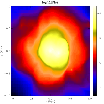
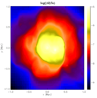
Figure 1: The logarithms of the intensity maps $|\Delta I|/I_{0}$ of the SZ effect at frequency of 150 GHz (upper) and 217 GHz (lower) derived from the numerical simulation in the framework of the Wright formalism.

In this paper we shall not consider SZ effects due to the motion of galaxy clusters, we note that the kinematic SZ effect can be extracted from the SZ intensity map at 217 GHz by using the method proposed in Sect. 5.1 by Prokhorov et al. (2010b).

In the next section, using the derived SZ intensity maps at frequencies of 150 GHz and 217 GHz, we show how to analyze the 3D temperature structure of galaxy clusters.

3 Unveiling the 3D temperature structure of galaxy clusters

The methods previously used in other papers permit us to derive 2D temperature maps of galaxy clusters. In this section, we propose a method to derive the standard temperature deviation and temperature variance along the line-of-sight for relatively cool galaxy clusters with temperatures less than 10 keV, which provides us with a tool to study the 3D temperature structure of merging galaxy clusters by means of the SZ effect.

Apart from the Wright formalism, there is another formalism to describe the relativistically correct SZ effect based on an extension of the Kompaneets equation which allows relativisitic effects to be included (Challinor & Lasenby 1998; Itoh et al. 1998). Analytical forms for the spectral changes due to the SZ effect, correct to first and second order in the expansion parameter $\Theta=k_{\mathrm{b}}T_{\mathrm{e}}/(m_{\mathrm{e}}c^{2})$, are given in Challinor & Lasenby (1998). We use the Wright formalism for calculating the SZ intensity maps from the simulation as accurately as possible and apply the formalism based on an extension of the Kompaneets equation to calculate the temperature variance along the line-of-sight, because it is the only one that can be manipulated in such a way as to derive this quantity.

We are focusing on studying relatively cool clusters with temperatures less than 10 keV because the SZ first order correction to the Kompaneets approximation is sufficient in this temperature range to calculate the SZ effect with a good precision (i.e. the SZ second order correction is very small).

The formalism based on an extension of the Kompaneets equation is obtained by solving the Boltzmann equation using the limitations of the single scattering approximation. Thus, the Boltzmann equation (see Challinor & Lasenby 1998) can only be applied to describe the SZ effect in optically thin clusters. The single scattering approximation is usually sufficient to calculate the SZ effect in galaxy clusters. We have checked that the single scattering approximation is valid for the considered simulated cluster.

To derive the temperature variance we propose to measure the SZ effect at two frequencies for disentangling the SZ relativistic correction from the SZ contribution which can be described by the Kompaneets approximation. The easiest way to do this is to choose one frequency at 217 GHz (i.e. the crossover frequency of the SZ effect in the Kompaneets approximation) and another frequency at which the SZ effect is described by the Kompaneets approximation. The SZ relativistic corrections are very small compared with the total SZ signal for relatively cool clusters at frequencies which are not close to the crossover frequency and are not very high (we have checked that the SZ relativistic corrections at frequencies of $\nu\gtrsim 540$ GHz are higher than 10% of the total thermal SZ effect for a galaxy cluster with $k_{\mathrm{b}}T_{\rm e}=5$ keV). At very high frequencies the contribution of SZ relativistic corrections is significant. Thus, we choose the second frequency at 150 GHz, which is a good choice since the modern experiments such as the Atacama Cosmology Telescope , Atacama Pathfinder Experiment telescope , and South Pole Telescope make SZ observations at this frequency.

The CMB intensity change produced by the SZ effect from a galaxy cluster with inhomogeneous density and temperature distributions in the formalism based on an extension of the Kompaneets equation, correct to first order in the expansion parameter $\Theta$, can be written as

$$\Delta I(x)\approx I_{\mathrm{0}}\sigma_{\mathrm{T}}\int n_{\mathrm{e}}\Theta\times(g(x)+\Theta\times g_{1}(x))dl,$$ (6)

where $g_{1}(x)$ is the spectral function taken from Eq. (28) of Challinor & Lasenby (1998) and is given by

$$g_{1}(x)=\frac{x^{4}\exp(x)}{(\exp(x)-1)^{2}}\left(-10+\frac{47}{2}x\coth(x/2)-\frac{42}{5}x^{2}\coth^{2}(x/2)+\right.$$

$$\left.\frac{7}{10}x^{3}\coth^{3}(x/2)+\frac{7x^{2}}{5\sinh^{2}(x/2)}\left(x\coth(x/2)-3\right)\right).$$ (7)

Since the optical depth of the electron plasma $\tau$ can be derived from X-ray observations or SZ observations, we rewrite Eq. (6) as

$$\Delta I(x)\approx I_{\mathrm{0}}\tau\left(\frac{\langle k_{\mathrm{b}}T_{\mathrm{e}}\rangle}{m_{\mathrm{e}}c^{2}}\times g(x)+\frac{\langle(k_{\mathrm{b}}T_{\mathrm{e}})^{2}\rangle}{m^{2}_{\mathrm{e}}c^{4}}\times g_{1}(x)\right),$$ (8)

where $\langle k_{\mathrm{b}}T_{\mathrm{e}}\rangle=\int n_{\mathrm{e}}k_{\mathrm{b}}T_{\mathrm{e}}dl/\int n_{\mathrm{e}}dl$ is the temperature averaged along the line-of-sight and $\langle(k_{\mathrm{b}}T_{\mathrm{e}})^{2}\rangle=\int n_{\mathrm{e}}(k_{\mathrm{b}}T_{\mathrm{e}})^{2}dl/\int n_{\mathrm{e}}dl$ is the squared temperature averaged along the line-of-sight.

As shown by Challinor & Lasenby (1998), for $k_{\mathrm{b}}T_{\mathrm{e}}=5$ keV, the second-order effects are very small over the entire intensity spectrum compared with the total thermal SZ effect. Therefore, we can use Eq.(8) to calculate approximately the SZ effect for the simulated cluster.

The SZ intensity at 150 GHz (x=2.64) is approximately given by the term of Eq.(8) proportional to $\langle k_{\mathrm{b}}T_{\mathrm{e}}\rangle$, since the SZ relativistic corrections at this frequency are very small compared with the total thermal SZ signal, i.e.

$$\Delta I(2.64)\approx I_{\mathrm{0}}\tau\frac{\langle k_{\mathrm{b}}T_{\mathrm{e}}\rangle}{m_{\mathrm{e}}c^{2}}\times g(2.64).$$

The SZ intensity at 217 GHz (x=3.83) is approximately given by the term of Eq.(8) proportional to $\langle(k_{\mathrm{b}}T_{\mathrm{e}})^{2}\rangle$, because the SZ relativistic corrections are a dominant contribution at this frequency, i.e.

$$\Delta I(3.83)\approx I_{\mathrm{0}}\tau\frac{\langle(k_{\mathrm{b}}T_{\mathrm{e}})^{2}\rangle}{m^{2}_{\mathrm{e}}c^{4}}\times g_{1}(3.83).$$

We note that both the temperature variance along the line-of-sight, which is given by

$$\mathrm{var}=\langle(k_{\mathrm{b}}T_{\mathrm{e}})^{2}\rangle-\langle k_{\mathrm{b}}T_{\mathrm{e}}\rangle^{2},$$ (9)

and the standard temperature deviation, which is given by

$$\sigma=\sqrt{\langle(k_{\mathrm{b}}T_{\mathrm{e}})^{2}\rangle-\langle k_{\mathrm{b}}T_{\mathrm{e}}\rangle^{2}},$$ (10)

can be derived for the simulated cluster from SZ observations at frequencies of 150 GHz (x=2.64) and 217 GHz (x=3.83). The temperature variance and standard temperature deviation for a homogeneous gas temperature distribution equal zero and, therefore, both the temperature variance and standard temperature deviation along the line-of-sight are a measure of inhomogeneity of the gas temperature along the line-of-sight.

In terms of the SZ intensities, the temperature variance along the line-of-sight is given by

$$\mathrm{var}\approx(m_{\mathrm{e}}c^{2})^{2}\left(\frac{\Delta I_{\mathrm{217GHz}}}{I_{0}\tau g_{1}(x=3.83)}-\left(\frac{\Delta I_{\mathrm{150GHz}}}{I_{0}\tau g(x=2.64)}\right)^{2}\right),$$ (11)

where $\Delta I_{\mathrm{150GHz}}$ and $\Delta I_{\mathrm{217GHz}}$ are the SZ intensities at frequencies of 150 GHz (x=2.64) and 217 GHz (x=3.83), respectively. The standard temperature deviation can be derived from SZ intensities at frequencies of 150 GHz and 217 GHz by using Eq. (11) and the relation between the temperature variance and standard temperature deviation, $\rm var=\sigma^{2}$.

We calculate the map of the standard temperature deviation along the line-of-sight using Eqs. (9), (10), and (11) and the SZ intensity maps at frequencies of 150 GHz and 217 GHz derived in the framework of the Wright formalism in Sect. 2. The map of the standard temperature deviation along the line-of-sight is shown in Fig. 2 (middle left-hand panel).

We note that the values of the standard temperature deviation are high in regions of high temperature on the SZ-temperature map, which is shown in Fig. 2 (top left-hand panel). The standard temperature deviation map contains high temperature “arc-like” structures, which are also seen in the temperature map. As noted by Prokhorov et al. (2010b), the origin of these “arc-like” structures is the major merger of two galaxy clusters occurring at z=0.8. Dubois et al. (2010) demonstrates that this major merger drives the cluster gas to temperatures twice the virial temperature thanks to violent merger shock waves.

The middle left-hand panel in Fig. 2 shows that the standard temperature deviation values in the regions of shock waves are $\simeq$50% of those of the gas temperature. The increase of the standard temperature deviation in the “arc-like” regions compared with other regions shows the presence of temperature inhomogeneities along the line-of-sight in these regions.

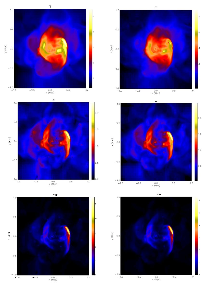
Figure 2: Maps of the Compton-average electron temperature in keV (top left-hand panel), mass-weighted temperature in keV (top right-hand panel), standard temperature deviation along the line-of-sight in keV derived from Eq. 11 (middle left-hand panel), standard temperature deviation along the line-of-sight in keV derived from 3D gas temperature and density distributions (middle right-hand panel), temperature variance in keV² along the line-of-sight derived from Eq. 11 (bottom left-hand panel), and temperature variance in keV² along the line-of-sight derived from 3D gas temperature and density distributions (bottom right-hand panel). All the maps are calculated for the simulated relatively cool galaxy cluster at z=0.74.

Our analysis of the standard temperature deviation map shows that the standard temperature deviation increases in the post-shock regions. Shock waves are places of significant gas heating, therefore they are interesting targets for analyzing by means of the temperature variance which is sensitive to the presence of temperature inhomogeneities. Using the calculated SZ intensity maps at frequencies of 150 GHz and 217 GHz and applying Eq. (11), we derive the temperature variance map of the simulated cluster. The temperature variance map is shown in Fig. 2 (bottom left-hand panel). Since the temperature variance equals the squared standard temperature deviation, the regions of high values of the standard temperature deviation are revealed with a higher contrast on the temperature variance map than with that on the standard temperature deviation map. Therefore, an analysis of the temperature variance map is a way to reveal shock fronts in merging galaxy clusters.

We conclude that the standard temperature deviation and temperature variance are sensitive to the gas temperature distribution along the line-of-sight and permit us to analyze the 3D temperature structure, and to reveal merger shock waves in galaxy clusters. We have demonstrated that the high temperature “arc-like” structures in the temperature maps shown in Fig. 2 (top panels) correspond to high values of the temperature variance along the line-of-sight.

4 Extending the proposed method: higher accuracy and hot clusters

In the previous section, we have demonstrated how to derive the standard temperature deviation and temperature variance along the line-of-sight using the Wright formalism and analytical forms for the spectral changes due to the SZ effect, correct to first order in the expansion parameter $\Theta$. In this section, we discuss some of the limitations of the proposed method, which arise from the use of analytical forms for the spectral changes correct to first order. To find the limitations of the proposed method, we calculate the standard temperature deviation and temperature variance maps using the simulated 3D gas density and temperature distributions.

The map of the standard temperature deviation along the line-of-sight, calculated by using the simulated 3D gas temperature and density distributions instead of the SZ intensities at frequencies of 150 GHz and 217 GHz, is plotted in Fig. 2 (middle right-hand panel). Comparing the standard temperature deviation maps plotted in Fig. 2 (middle panels) shows that the maximal difference between these standard temperature deviation maps is around 8%. Therefore, we conclude that the standard temperature deviation along the line-of-sight derived from the method proposed in the previous section is in good agreement with the true standard temperature deviation along the line-of-sight.

The temperature variance map derived from the 3D gas temperature and density distributions instead of the SZ intensities is shown in Fig. 2 (bottom right-hand panel). The maximal difference between the values of the temperature variance derived from the SZ intensities (see the bottom left-hand panel in Fig. 2) and from the simulated 3D gas temperature and density distributions (see the bottom right-hand panel in Fig. 2) is around 15%. We propose below how to calculate the variance map by means of the SZ effect more accurately.

Although the second-order correction is very small compared with the total SZ effect for relatively cool galaxy clusters, this correction leads to a $\simeq 10\%$ (average) uncertainty on the temperature variance map. To improve the agreement between the true and derived temperature variance maps, we propose to use a combined generalized spectral function proposed in Prokhorov et al. (2010a). Since there is a small contribution to the SZ signal at a frequency of 217 GHz, derived in the formalism based on an extension of the Kompaneets equation, from the second-order effects, we propose to exclude this contribution by using SZ observations at two frequencies at which the second-order effects equal to zero. Using Eq. (33) from Challinor & Lasenby (2010), we find that the second-order effects are equal to zero at frequencies of 197 GHz (x=3.47) and 397 GHz (x=7.0). Therefore, the combined generalized spectral function, which corresponds to a relativistic contribution to the generalized function at a frequency of 197 GHz taking into account a measurement at a frequency 397 GHz and is defined in Eq. (7) of Prokhorov et al. (2010a), is determined by the first-order effects and does not depend on the zero-order and second-order effects. If SZ observations at these frequencies are used to derive the signal of $\Delta I_{\mathrm{197GHz}}-\Delta I_{\mathrm{397GHz}}\times g(x=3.47)/g(x=7.0)$, which does not depend on the zero-order and second-order effects, this permits us to use this SZ signal instead of the SZ signal at 217 GHz to improve the agreement between the true and derived temperature variance maps. Note that the third-order corrections are negligible over the entire spectrum for $k_{\mathrm{b}}T_{\mathrm{e}}\lesssim 10$ keV (Challinor & Lasenby 1998). We have checked that the contribution of the third-order corrections to the signal of $\Delta I_{\mathrm{197GHz}}-\Delta I_{\mathrm{397GHz}}\times g(x=3.47)/g(x=7.0)$ is much smaller than the contribution of the second-order corrections to the SZ signal at a frequency of 217 GHz. The use of the combined generalized spectral function permits us to extend the proposed method to hot galaxy clusters with gas temperatures in the range of 10 keV – 15 keV (see Sect. 5).

The method to derive the first-order SZ correction by using SZ observations at frequencies of 197 GHz and 397 GHz is more observationally complex than that based on measuring the SZ signal at the crossover frequency of 217 GHz. This is because the contamination by point-like sources is lower at 217 GHz than that at 397 GHz and because the 150 GHz and 217 GHz atmospheric windows are easier for observing from the ground (i.e. the atmosphere is more transparent at 150 GHz and 217 GHz). Therefore, the method based on measuring the SZ signal at 217 GHz is more suitable for relatively cool galaxy clusters with $k_{\mathrm{b}}T_{\mathrm{e}}\lesssim 10$ keV. The advantage of the method based on measuring the SZ signals at 197 GHz and 397 GHz is that it provides us with a possibility to measure the temperature variance in hot galaxy clusters with $k_{\mathrm{b}}T_{\mathrm{e}}$ in the range of 10 keV – 15 keV.

We conclude that the maps of the standard temperature deviation and temperature variance derived in Sect. 3 are close to the true maps derived from 3D gas temperature and density distributions. Therefore, the maps of the temperature variance and standard temperature deviation derived from SZ observations at frequencies of 150 GHz and 217 GHz are promising to analyze the 3D temperature structure of galaxy clusters and to reveal the merger shocks in galaxy clusters.

An analysis of the standard temperature deviation and temperature variance along the line-of-sight by means of the SZ effect will permit us to improve the deprojection technique of merging galaxy clusters. The deprojection of temperature maps is so far based on symmetry assumptions, since the quantities integrated along the line-of-sight are involved. The use of the standard temperature deviation and temperature variance, which are measure of gas inhomogeneity along the line-of-sight, provides us with a possibility to be independent from symmetry assumptions and to obtain more realistic deprojection temperature maps.

Shock fronts are places of gas heating and, therefore, the gas temperature inhomogeneities along the line-of-sight are large near shock fronts. Studying the temperature variance map provides us with a new independent approach to unveil shock fronts in merging galaxy clusters.

5 Studying the 3D temperature structure of hot galaxy clusters

We now demonstrate how to derive the temperature variance along the line-of-sight for hot galaxy clusters with gas temperatures in the range of 10 keV – 15 keV by using the improved method proposed in the previous section. To produce the SZ intensity maps at frequencies of 150 GHz, 197 GHz, and 397 GHz, we use the 3D numerical simulations of the merging hot galaxy cluster presented in Akahori & Yoshikawa (2010).

The simulations of merging galaxy clusters by Akahori & Yoshikawa (2010) are carried out using an N-body and SPH code developed in Akahori & Yoshikawa (2008), which adopts the entropy–conservative formulation of SPH by Springel & Hernquist (2002), and the standard Monaghan-Gingold artificial viscosity (Monaghan & Gingold 1983) with the Balsara limiter (Balsara 1995). They carried out an adiabatic run in which radiative cooling, star formation, and AGN feed back are not taken into consideration.

In the simulations, an encounter of two free-falling galaxy subclusters from the epoch of their turn-around is considered. The two galaxy subclusters have virial masses and radii of $M_{\mathrm{200},1}=8\times 10^{14}M_{\odot}$ and $r_{\mathrm{200},1}=1.91$ Mpc, and $M_{\mathrm{200},2}=2\times 10^{14}M_{\odot}$ and $r_{\mathrm{200},2}=1.21$ Mpc, respectively, where $r_{\rm 200}$ is the radius within which the mean cluster mass density is 200 times the present cosmic critical density. The initial distributions of a dark matter halo and a ICM component are the NFW density profile (Navarro et al. 1997) and the $\beta$-model density profile (Cavaliere & Fusco-Femiano 1976), respectively. The scale radius of the NFW profile is set to $r_{\rm s}=r_{\rm 200}/5.16$, and the core radius of the $\beta$-model is $r_{\rm c}=r_{\rm s}/2$.

The massive subcluster is composed of one million dark matter particles and the same number of SPH particles, while the less massive subcluster is represented by a quarter million particles for each component. The corresponding spatial resolution (the smoothing length) of SPH is $\sim 50$ kpc at the ICM density of $10^{-3}{\rm cm^{-3}}$. We use the result with zero impact parameter at a time of $t=0.5$ Gyr, where $t=0$ Gyr corresponds to the time of the closest approach of the centers of the dark matter halos. The average temperature of this simulated galaxy cluster is $\simeq$ 10 keV and the temperature of the hottest regions associated with shock fronts is $\simeq$ 15 keV. For further details of the simulation, see Akahori & Yoshikawa (2010).

The dense cores of these two subclusters are accelerated by the preceding dark matter halos and shock waves are formed in front of the cores. Shock fronts are shown in the Mach number distribution plotted in Fig. 2 of Akahori & Yoshikawa (2010). Since the temperature and density maps of the simulated hot merging cluster are inhomogeneous owing to the presence of shock waves, we study the map of the temperature variance along the line-of-sight for this cluster.

For a hot galaxy cluster with inhomogeneous density and temperature ($k_{\rm{b}}T_{\rm{e}}\leq 15$ keV) distributions, the CMB intensity change produced by the SZ effect in the formalism based on an extension of the Kompaneets equation, which is correct to second order in the expansion parameter $\Theta$, can be written as

$$\Delta I(x)\approx I_{\mathrm{0}}\sigma_{\mathrm{T}}\int n_{\mathrm{e}}\Theta\times(g(x)+\Theta\times g_{1}(x)+\Theta^{2}\times g_{2}(x))dl$$ (12)

where $g(x)$, $g_{1}(x)$, and $g_{2}(x)$ are the spectral functions taken from Challinor & Lasenby (1998). Note that higher order terms should be included for calculating the SZ effect from very hot galaxy clusters with $k_{\rm{b}}T_{\rm{e}}\geq 15$ keV (e.g. Challinor & Lasenby 1998; Itoh et al. 1998). Since the optical depth $\tau$ of the electron plasma can be derived from X-ray or SZ observations, we rewrite Eq. (12) as

$$\Delta I(x)\approx I_{\mathrm{0}}\tau\left(\frac{\langle k_{\mathrm{b}}T_{\mathrm{e}}\rangle}{m_{\mathrm{e}}c^{2}}\times g(x)+\frac{\langle(k_{\mathrm{b}}T_{\mathrm{e}})^{2}\rangle}{m^{2}_{\mathrm{e}}c^{4}}\times g_{1}(x)+\right.$$ (13)

$$\left.\frac{\langle(k_{\mathrm{b}}T_{\mathrm{e}})^{3}\rangle}{m^{3}_{\mathrm{e}}c^{6}}\times g_{2}(x)\right),$$

In terms of the SZ intensities, the temperature variance along the line-of-sight is given by

$$\mathrm{var}=(m_{\mathrm{e}}c^{2})^{2}\left(\frac{\Delta\tilde{I}_{\mathrm{197GHz},\mathrm{397GHz}}}{I_{0}\tau\tilde{g}}-\left(\frac{\Delta I_{\mathrm{150GHz}}}{I_{0}\tau g(x=2.64)}\right)^{2}\right),$$ (14)

where $\Delta I_{\mathrm{150GHz}}$ is the SZ intensity at a frequency of 150 GHz (x=2.64), $\Delta\tilde{I}_{\mathrm{197GHz},\mathrm{397GHz}}$ is the combined SZ intensity at frequencies of 197 GHz (x=3.47) and 397 GHz (x=7.0), which is defined as (Prokhorov et al. 2010a)

$$\Delta\tilde{I}_{\mathrm{197GHz},\mathrm{397GHz}}=\Delta I_{\mathrm{197GHz}}-\Delta I_{\mathrm{397GHz}}\times\frac{g(x=3.47)}{g(x=7.0)},$$ (15)

and $\tilde{g}$ is the coefficient which equals

$$\tilde{g}=g_{1}(x=3.47)-g_{1}(x=7.0)\times\frac{g(x=3.47)}{g(x=7.0)}.$$ (16)

The map of the standard temperature deviation along the line-of-sight derived from our mock SZ observations at frequencies of 150 GHz, 197 GHz, and 397 GHz is shown in Fig. 3 (top panel).

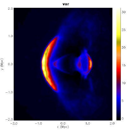
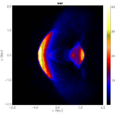
Figure 3: Maps of the temperature variance in keV² along the line-of-sight derived from Eq. 14 (top panel) and from 3D gas temperature and density distributions (bottom panel)

The map of the temperature variance, calculated by using the simulated 3D gas temperature and density distributions instead of the SZ intensities at frequencies of 150 GHz, 197 GHz, and 397 GHz, is plotted in Fig. 3 (bottom panel). Comparing the maps in Fig. 3 shows that the maximal difference between these maps is $\approx$ 25%. Measurements of the temperature variance by means of the proposed method permit us to study temperature inhomogeneities along the line-of-sight. We find that the values of the the temperature variance are high in the post-shock regions and, therefore, the map of this quantity can also be used to unveil merger shocks in hot galaxy clusters.

We will study possibilities of deriving the temperature variance along the line-of-sight for hot merging galaxy clusters by means of the planned SZ experiments in a forthcoming paper.

6 Conclusions

A number of important gasdynamic processes can be studied by observing merging galaxy clusters. Studying the temperature structure of merging clusters is important to reveal heated regions associated with merger shock waves and is complicated because the temperature maps of merging clusters are very inhomogeneous and because the approximation of a spherically symmetric gas distribution is not suitable for merging galaxy clusters. In many merging clusters, such as the Abell 3376 cluster (see Bagchi et al. 2007), the temperature distribution is very inhomogeneous and it is possible to derive only the 2D temperature map.

In this paper we demonstrate how to derive the quantities describing the temperature distribution along the line-of-sight for relatively cool merging galaxy clusters with $k_{\mathrm{b}}T_{\mathrm{e}}\lesssim 10$ keV. To produce a realistic merging cluster, we have used a zoomed cosmological simulation from Dubois et al. (2010) and found that the simulated galaxy cluster undergoes a violent merger. The temperature map of the simulated cluster becomes very inhomogeneous because of the merger activity. We have incorporated the relativistic Wright formalism for modeling the SZ effect in the numerical simulation using the algorithm proposed by Prokhorov et al. (2010a). We calculated the SZ intensity maps at frequencies of 150 GHz and 217 GHz.

We propose a method to derive the standard temperature deviation and temperature variance along the line-of-sight using SZ observations at frequencies of 150 GHz and 217 GHz. We found that the values of the standard temperature deviation in the regions of shock waves are around 50% of those of the gas temperature. The increase of the values of the standard temperature deviation in the “arc-like” regions, which were studied by Prokhorov et al. (2010b), compared with other regions shows the presence of temperature inhomogeneity along the line-of-sight in the “arc-like” regions. Using the 3D gas temperature and density distributions in the simulated galaxy cluster, we have checked that the map of the standard temperature deviation derived by means of the proposed method based on SZ observations is in agreement with the true map of the standard temperature deviation.

We show that the temperature variance along the line-of-sight is an useful quantity which provides us with a possibility to reveal merger shock waves in galaxy clusters. We calculated this quantity by using SZ observations at frequencies of 150 GHz and 217 GHz. The “arc-like” structures are revealed with a much higher contrast in the map of this quantity than that in the map of the standard temperature deviation and shock fronts can be observed by measuring this quantity. Therefore, an analysis of maps of the temperature variance is interesting to reveal merger shock waves in galaxy clusters.

We extend our method and make it applicable to hot merging galaxy clusters with gas temperatures in the range of 10 keV – 15 keV in Sect. 4. Using the data of numerical simulations of Akahori & Yoshikawa (2010), we demonstrate how to derive the temperature variance along the line-of-sight for the simulated hot merging cluster of galaxies in Sect. 5.

Our study demonstrates that the SZ effect is a promising tool to reveal the 3D temperature structure of galaxy clusters. We have proposed the method which provides us with the possibility of an analysis of the temperature distribution along the line-of-sight.

References

- [1] Akahori, T., & Yoshikawa, K. 2008, PASJ, 60, L19
- [2] Akahori, T., Yoshikawa, K. 2010, PASJ, 62, 335
- [3] Bagchi, J., Durret, F., Lima Neto, G. B., & Paul, S. 2006, Science, 314, 791
- [4] Balsara, D. S. 1995, J. Comput. Phys., 121, 357
- [5] Birkinshaw, M. 1999, Phys. Rep., 310, 97
- [6] Cavaliere, A., & Fusco-Femiano, R. 1976, A&A, 49, 137
- [7] Challinor, A., Lasenby, A. 1998, ApJ, 499, 1
- [8] Colafrancesco, S., Marchegiani, P. 2010, A&A, 520, 31
- [9] Dubois, Y., Teyssier, R. 2008, A&A, 477, 79
- [10] Dubois, Y., Devriendt, J., Slyz, A., Teyssier, R. 2010, MNRAS, 409, 985
- [11] Gitti, M., O’Sullivan, E., Giacintucci, S. et al. 2010, ApJ, 714, 758
- [12] Haardt F., Madau P., 1996, ApJ, 461, 20
- [13] Hansen, S. H., Pastro, S., Semikoz, D. V. 2002, ApJ, 573, L69
- [14] Itoh, N., Kohyama, Y., Nozawa, S. 1998, ApJ, 502, 7
- [15] Kay, S. T., Powell, L. C., Liddle, A. R., & Thomas, P. A. 2008, MNRAS, 386, 2110
- [16] Kompaneets, A. S. 1957, Soviet Phys. – JETP, 4, 730
- [17] Markevitch, M. et al. 2002, ApJ, 567, L27
- [18] Markevitch, M., Vikhlinin, A. 2007, Phys. Rep., 443, 1
- [19] Monaghan, J. J., & Gingold, R. A. 1983, J. Comput. Phys., 52, 374
- [20] Navarro, F. J., Frenk, C. S, & White, S. D. M. 1997, ApJ, 490, 493
- [21] Pointecouteau, E., Giard, M., Barret, D. 1998, A&A, 336, 44
- [22] Prokhorov, D. A., Antonuccio-Delogu, V., Silk, J. 2010a, A&A, 520, A106
- [23] Prokhorov, D. A., Dubois, Y., Nagataki, S. 2010b, A&A, 524, A89
- [24] Rasera Y., Teyssier R., 2006, A&A, 445, 1
- [25] Sarazin, C. L. 1986, Rev. Mod. Phys., 58, 1
- [26] Spergel D. N. et al., 2003, ApJS, 148, 175
- [27] Springel, V., & Hernquist, L. 2002, MNRAS, 333, 649
- [28] Sunyaev, R. A., Zel’dovich, Ya. B. 1980, ARA&A, 18, 537
- [29] Teyssier, R. 2002, A&A, 385, 337
- [30] Wright, E. L. 1979, ApJ, 232, 348