Enhanced spin transfer torque effect for transverse domain walls in cylindrical nanowires

Abstract

Recent studies have predicted extraordinary properties for transverse domain walls in cylindrical nanowires: zero depinning current, the absence of the Walker breakdown, and applications as domain wall oscillators. In order to reliably control the domain wall motion, it is important to understand how they interact with energy barriers, which may be engineered for example through modulations in the nanowire geometry (such as notches or extrusions) or as inhomogeneities in the material’s crystal anisotropy.

In this paper, we study the motion and depinning of transverse domain walls through potential barriers in ferromagnetic cylindrical nanowires. We use (i) magnetic fields and (ii) spin-polarized currents to drive the domain walls along the wire. Barriers are modelled as a section of the nanowire which exhibits a uniaxial crystal anisotropy where the anisotropy easy axis and the wire axis enclose a variable angle $\theta_{\mathrm{P}}$. Using (i) magnetic fields, we find that the minimum and the maximum fields required to push the domain wall through the barrier differ by $30\%$. On the contrary, using (ii) spin-polarized currents, we find variations of a factor 130 between the minimum value of the depinning current density (observed for $\theta_{\mathrm{P}}=0^{\circ}$, i.e. anisotropy axis pointing parallel to the wire axis) and the maximum value (for $\theta_{\mathrm{P}}=90^{\circ}$, i.e. anisotropy axis perpendicular to the wire axis).

We study the depinning current density as a function of the height of the energy barrier using numerical and analytical methods. We find that for an industry standard energy barrier of $40\,k_{\mathrm{B}}T$, a depinning current density of about $5\,\mu A$ (corresponding to a current density of $6\times 10^{10}\,\mathrm{A/m}^{2}$ in a nanowire of $10\,\mathrm{nm}$ diameter) is sufficient to depin the domain wall.

We reveal and explain the mechanism that leads to these unusually low depinning currents. One requirement for this new depinning mechanism is for the domain wall to be able to rotate around its own axis. With the right barrier design, the spin torque transfer term is acting exactly against the damping in the micromagnetic system, and thus the low current density is sufficient to accumulate enough energy quickly. These key insights may be crucial in furthering the development of novel memory technologies, such as the racetrack memory, that can be controlled through low current densities.

I Introduction

The current induced motion of domain walls (DWs) in ferromagnetic nanowires has been the subject of intense study in recent years. Being able to move and control DWs accurately is an important step towards the realisation of devices such as the racetrack memory Parkin2008 . Two main challenges are the high critical current density, $j_{\mathrm{D}}$, required to depin the DW and initiate the DW motion Tatara2004 and the so-called Walker breakdown, a phenomenon which limits the DW velocity and is caused by deformations in the magnetization structure Klaui2005 . It has been recently observed Yan2010 ; Wieser2010 that transverse domain walls (TDWs) in cylindrical nanowires are not subject to such limitations: $j_{\mathrm{D}}$ is zero, and the Walker breakdown does not occur. These DWs are able to propagate uniformly, without any deformation of their internal structure. Moreover, recent theoretical studiesfranchin2008jap ; Franchin2008prb ; Ono2008 suggest that TDWs may play an important role in the emerging research area of domain wall oscillatorsHe2007 ; Matsushita2009 ; Bisig2009 ; Finocchio2010 ; Masaaki2011 (DWOs), providing an effective way to sustain magnetization dynamics with direct currents.

The main obstacle for the experimental observation of these effects is that TDWs only occur in cylindrical nanowires with small diameter (below $\sim 50\,\mathrm{nm}$ for Permalloy). In wires with greater diameter the demagnetizing field is strong enough to force the magnetization to follow the cylindrical surface of the wire, thus changing the internal structure of the DW, giving rise to a vortex DWWieser2004 ; Yan2010 . As a consequence, the experimental validation of the predicted properties of TDW requires the fabrication of cylindrical nanowires with diameter below $50\,\mathrm{nm}$, which is challenging from an experimental point of view. Recently, however, novel techniques have been developed for fabricating cylindrical nanowires with small diameter Cao2001 ; Ruitao2007 ; Pitzschel2011a . Ruitao et. al.Ruitao2007 describe a procedure to obtain single crystalline Permalloy nanowires with an average diameter of $\sim 30\,\mathrm{nm}$, through in situ filling of the inner cavities of carbon nanotubes. Pitzschel et. al.Pitzschel2011a discuss the fabrication of arrays of Ni cylindrical nanowires with diameter between $80$ and $160\,\mathrm{nm}$, using electrodeposition. Such arrays are technologically relevant, as they may represent a practical and convenient way to densely pack nanowires for memory storage applications. In particular, the authors discuss how the diameter of the nanowires can be modulated in order to introduce geometrical “artifacts” which act as barriers for the propagation of DWs. These barriers may be necessary in order to control the DW motion and make it more predictable and reliable. It is then important for technological applications to study and understand the motion of TDWs through obstacles (which may be realized as inhomogeneities in the material or in the geometry in the nanowire).

In this paper we present a micromagnetic study of the field-driven and current-driven motion of transverse domain walls through potential barriers in cylindrical nanowires. We consider two kinds of barriers: cylindrically symmetric barriers, whose associated energy term is invariant for rotations of the magnetization around the nanowire axis, and cylindrically asymmetric barriers, whose energy term does depend on the rotational state of the magnetization. When passing through a cylindrically symmetric barrier the TDW is “rotationally-free”, i.e. it can rotate freely around the nanowire axis. On the contrary, when passing through a cylindrically asymmetric barrier the TDW is “rotationally-bound”, as the barrier introduces an energy penalty for rotations of the DW. We find that the current density required to push the DW through the barrier is radically different in the two cases. In particular, we report that current densities of $10^{10}-10^{11}\,\mathrm{A/m}^{2}$ can be used to depin rotationally-free DWs from barriers which are thermally “stable” at room temperature (the associated energy is greater than $40\,k_{\mathrm{B}}T$ at $T=300\,\mathrm{K}$). In contrast, depinning a rotationally-bound DW requires current densities which are higher by a factor $\sim 130$.

II The system

In order to study the field-driven and current-driven motion of a DW through a potential barrier, we employ the system schematically shown in Fig. 1, a long cylindrical ferromagnetic nanowire.

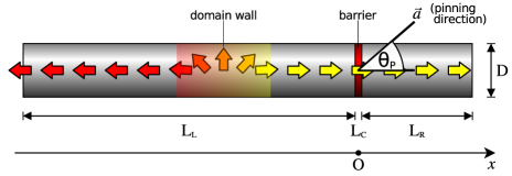
Figure 1: (Color online) Sketch of the system. The arrows on the cylinder axis represent the magnetization. The transverse DW on the left is pushed through the barrier on the right. The barrier is modeled as a region where an additional uniaxial anisotropy pins the magnetization along the direction determined by $\theta_{\mathrm{P}}$.

The potential barrier is modeled as a thin region of the wire of length $L_{\mathrm{C}}$ where a uniaxial anisotropy pins the magnetization along a given direction $\vec{a}$ with a given strength $K_{1}$. In this first part of the paper, we fix the value of the anisotropy constant $K_{1}$ and study how the motion of the DW depends on $\theta_{\mathrm{P}}$, the angle between the unit vector $\vec{a}$ and the nanowire axis.

The nanowire is subdivided into three regions: one longer region on the left with length $L_{\mathrm{L}}$ and one shorter region on the right with length $L_{\mathrm{R}}$, separated by the barrier, a thin layer of width $L_{\mathrm{C}}$. In the simulation we “place” a DW on the left of the barrier and try to push it to the right using increasing applied fields (Sec. III) or current densities (Sec. IV).

The dynamics of the magnetization, $\vec{M}$, is computed using the Landau-Lifshitz equation, extended with two additional terms in order to model spin transfer torque effects ZhangLiModel2004 :

$$\partial_{t}\vec{M} = -\gamma\,\vec{M}\times\vec{H}+\frac{\alpha}{M_{\mathrm{s}}}\,\vec{M}\times\partial_{t}\vec{M}$$ (1)

$${}+v\,\partial_{x}\vec{M}-\frac{\xi v}{M_{\mathrm{s}}}\,\vec{M}\times\partial_{x}\vec{M}$$

In this equation, $M_{\mathrm{s}}=\|\vec{M}\|$ is the saturation magnetization, $\vec{H}$ is the effective magnetic field, $\gamma$ is the gyromagnetic ratio, $\alpha$ is the damping parameter. The current density, $j_{\mathrm{app}}$, is applied along the $x$ direction and enters the model through the parameter $v=\frac{Pj_{\mathrm{app}}\mu_{B}}{eM_{\mathrm{s}}(1+\xi^{2})}$, where $P$ is the degree of polarization of the spin current, $\mu_{B}$ is the Bohr magneton, $e$ the absolute value of the electron charge, $\xi$ the non-adiabatic parameter. Note that in this paper we reason in terms of fully polarized current densities, $j=Pj_{\mathrm{app}}$, rather than in terms of the actual applied current densities, $j_{\mathrm{app}}$.

The effective field is calculated as $\vec{H}=\vec{H}_{\mathrm{exch}}+\vec{H}_{\mathrm{demag}}+\vec{H}_{\mathrm{app}}+\vec{H}_{\mathrm{pin}}$, where $\vec{H}_{\mathrm{exch}}=\frac{2A}{\mu_{0}M_{\mathrm{s}}}\,\nabla^{2}\vec{m}$ is the exchange field, $\vec{H}_{\mathrm{demag}}$ is the magnetostatic field, $\vec{H}_{\mathrm{app}}$ is the applied field and $\vec{H}_{\mathrm{pin}}=(2K_{1}\vec{m}\cdot\vec{a}/\mu_{0}M_{\mathrm{s}})\,\vec{a}$ is the magnetic anisotropy corresponding to the pinning potential $U_{\mathrm{pin}}=-K_{1}\,(\vec{m}\cdot\vec{a})^{2}$. $K_{1}$ is the only parameter which varies in space: it is zero outside the barrier region, and is set to $K_{1}=0.5\times 10^{6}\,\mathrm{J}/\mathrm{m}^{3}$ inside it. The other parameters are homogeneous throughout the whole nanowire and are set to $M_{\mathrm{s}}=0.86\times 10^{6}\,\mathrm{A/m}$, $A=1.3\times 10^{-11}\,\mathrm{A/m}$, $\gamma=2.21\times 10^{5}\,\mathrm{m}/(\mathrm{As})$, $\alpha=0.01$ and $\xi=0.01$, which are typical values for Permalloy. Concerning the geometry of the cylindrical nanowire we take $L_{\mathrm{L}}=148.5\,\mathrm{nm}$, $L_{\mathrm{R}}=48.5\,\mathrm{nm}$, $L_{\mathrm{C}}=3\,\mathrm{nm}$, so that the total length is $L=L_{\mathrm{L}}+L_{\mathrm{C}}+L_{\mathrm{R}}=200\,\mathrm{nm}$. The diameter is chosen as $D=10\,\mathrm{nm}$. Contributions from the Oersted field and the Joule heating are negligible for nanowires of small radiusFranchin2008prb and are thus not included in the model.

We note that, when $\theta_{\mathrm{P}}>0^{\circ}$, the pinning field $\vec{H}_{\mathrm{pin}}$ tries to pull the magnetization out of the axis of the nanowire. The magnetostatic field, however, opposes this and — for the value of $K_{1}$ considered in this paper — manages to keep the magnetization along the axis of the nanowire, even inside the potential barrier.

Eq. (1) is discretized over a finite element mesh and the simulations are carried out using a version of the micromagnetic simulation package Nmag Fischbacher2007a ; nmag2006 , extended to model spatially varying magnetic anisotropies.

III Field-driven DW motion

We carry out a number of simulations to determine the critical field, $H_{\mathrm{crit}}$, which must be applied (in the direction of the nanowire axis) in order to push the DW through the potential barrier. In particular, we fix the pinning strength to $K_{1}=0.5\times 10^{6}\,\mathrm{J}/\mathrm{m}^{3}$ and perform one simulation for each value of the pinning angle $\theta_{\mathrm{P}}$, which is changed from zero (pinning along the nanowire axis) to $90^{\circ}$ (pinning orthogonal to the nanowire axis) in steps of $5\,^{\circ}$.

Each simulation is carried out in two parts. In the first part, a preliminary relaxation computation is carried out and the system settles into a metastable state where a DW is located on the left of the barrier. In the second part, the applied field is increased gradually until the DW passes through the barrier. For the preliminary relaxation we set the initial magnetization in the following way,

$$\vec{M}(x,y,z) = M_{\mathrm{s}}\,(\sin\theta(x),\,\cos\theta(x),\,0),$$ (2)

where $\theta(x)=\frac{\pi}{2}\min\left(1.0,\,\max\left(-1.0,\,\tiny(x-x_{0})/w\right)\right)$ and $x_{0}=-30\,\mathrm{nm}$, $w=20\,\mathrm{nm}$ (the reference system is chosen as in Fig. 1). For this choice of parameters, the magnetization relaxes into a tail-to-tail DW, located on the left of the nanowire, similarly to what is schematically shown in Fig. 1. The components of the magnetization along the axis of the nanowire before and after the relaxation computation are shown in Fig. 3. The relaxation is carried out using an artificially high value for the damping, $\alpha=0.5$, to speed up the computation, and is done in the presence of a small magnetic field, $H_{0}=10^{3}\,\mathrm{A}/\mathrm{m}$, which is applied along the negative $x$ direction and is used to push the DW towards the barrier. We want indeed to ensure that the DW settles into an equilibrium position against the barrier (e.g the center of the barrier) before starting to “depin” it. The convergence criterion used to stop the simulation is the following:

$$\max\left\{\frac{1}{M_{\mathrm{s}}}\left\|\frac{\mathrm{d}\vec{M}_{i}}{\mathrm{d}t}\right\|\right\}_{i}<\varepsilon$$ (3)

where the index $i$ runs over all the sites of the finite element mesh and $\varepsilon=1\,\mathrm{deg}/\mathrm{ns}$.

The procedure described above brings the system to a state which is different for different values of the pinning angle, $\theta_{\mathrm{P}}$. In particular, when $\theta_{\mathrm{P}}$ is zero the DW approaches the barrier from the left without penetrating it (Fig. 2(a).),

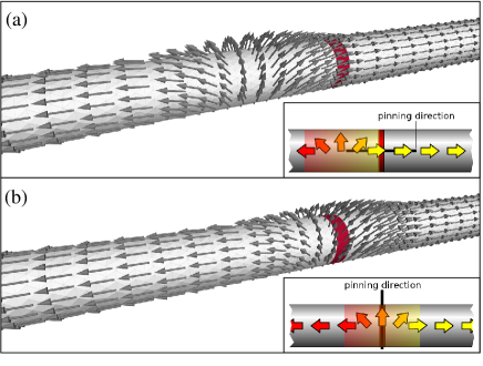
Figure 2: (Color online) The relaxed magnetization configurations for $\theta_{\mathrm{P}}=0^{\circ}$ (a) and $\theta_{\mathrm{P}}=90^{\circ}$ (b). The sketches on the corners of the two figures show that the DW moves into the barrier to allow the magnetization to align along the pinning direction in the barrier.

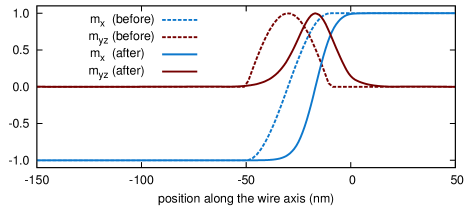
Figure 3: (Color online) The components of the normalized magnetization, $\vec{m}=\vec{M}/M_{\mathrm{s}}$, along the axis of the nanowire before (dashed lines) and after (solid lines) the preliminary relaxation computation. The blue curves (light in greyscale) show the $x$ (axial) component of $\vec{m}$, while the dark red curves (dark in greyscale) show the component of $\vec{m}$ orthogonal to the axis.

as this would require the magnetization in the region to move out of the pinning direction. On the other hand, when $\theta_{\mathrm{P}}$ is $90^{\circ}$ the DW “falls” into the center of the barrier allowing the magnetization to align along the pinning direction, with a consequent reduction in energy (see Fig. 2(b)). Depending on $\theta_{\mathrm{P}}$ we then have two different scenarios, where the barrier either repels the DW (as for $\theta_{\mathrm{P}}=0^{\circ}$) or attracts it (as for $\theta_{\mathrm{P}}=90^{\circ}$).

The magnetization configuration obtained from the preliminary relaxation computation is used as the initial state for the second part of the simulation, in which the damping is set to the realistic value, $\alpha=0.01$, and the applied field is gradually increased until the DW passes completely through the potential barrier. In particular, we increase the field in steps of $\Delta H=10^{2}\,\mathrm{A}/\mathrm{m}$ and for each value of the applied field we relax the system, i.e. perform a time integration of Eq. (1) until the convergence criterion (3) is met. To determine when the DW passes through the barrier and stop the simulation, we analyze the values of the spatially averaged normalized magnetization $\langle\vec{m}\rangle$, where $\vec{m}=\vec{M}/M_{\mathrm{s}}$. The $x$ component of this vector, $\langle m_{x}\rangle$, provides a good indication of the position of the DW, while the $y$ and $z$ components provide information about its state of rotation. In particular, if we assume the DW to be mirror-symmetric along the $x$ axis, we get $\langle m_{x}\rangle\approx(L_{\mathrm{R}}-L_{\mathrm{L}}-2x_{\mathrm{DW}})/L$, where $x_{\mathrm{DW}}$ is the position of the DW, while $L$ is the total length of the nanowire, $L=L_{\mathrm{L}}+L_{\mathrm{C}}+L_{\mathrm{R}}$. In the simulations we assume the DW to pass through the potential barrier when $\langle m_{x}\rangle<-0.75$, which corresponds, following the formula above, to a position of $x_{\mathrm{DW}}=25\,\mathrm{nm}$.

The results of the simulations are collected in Fig. 4.

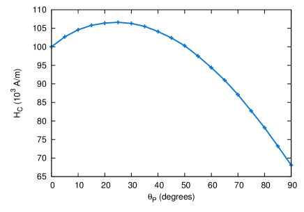
Figure 4: (Color online) $H_{\mathrm{crit}}$, the field required in order to push the DW throughout the potential barrier, is plotted as a function of the pinning angle, $\theta_{\mathrm{P}}$.

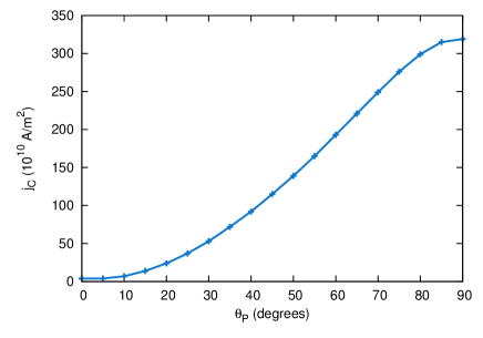
Figure 5: (Color online) $j_{\mathrm{crit}}$, the current required in order to push the DW through the potential barrier, is plotted as a function of the pinning angle, $\theta_{\mathrm{P}}$.

The field necessary to move the DW through the barrier varies between $(68.05\pm 0.05)$ and $(106.55\pm 0.05)\,\mathrm{kA}/\mathrm{m}$.

IV Current-driven DW motion

In order to determine the current necessary to push the DW through the barrier we follow a procedure analogous to the one described in the previous section, with two main differences. First, to push the DW we use a current rather than a field. Second, we abandon the convergence criterion in Eq. (3). This convergence criterion works well in the field-driven case because the torque is guaranteed to decrease in time due to the damping term. In the current-driven case, however, the spin transfer torque can oppose the damping and bring the system to a steady state where the magnetization dynamics is sustained in time. In particular, it may happen that the DW reaches a state where it does not advance anymore along the wire but keeps rotating around its axis Franchin2008prb . In this situation, the torque never falls below the given threshold, $\varepsilon$, and Eq. (3) is never satisfied. We then use a convergence criterion which stops the simulation when the DW translational velocity (along $x$) falls below a certain threshold. For convenience, we formulate it in terms of $\langle m_{x}\rangle$, as follows:

$$\left|\frac{\langle m_{x}(t+\Delta t)\rangle-\langle m_{x}(t)\rangle}{\Delta t}\right|<\varepsilon,$$ (4)

with $\varepsilon=10^{-5}\,\mathrm{ns}^{-1}$. The convergence criterion is checked every $\Delta t=100\,\mathrm{ps}$ and the simulation is stopped when it is satisfied for five consecutive times. We note that Eq. (4) may be expressed in terms of the DW velocity using the relation $\langle m_{x}\rangle=(L_{\mathrm{R}}-L_{\mathrm{L}}-2x_{\mathrm{DW}})/L$,

$$v_{\mathrm{DW}}=\left|\frac{x_{\mathrm{DW}}(t+\Delta t)-x_{\mathrm{DW}}(\Delta t)}{\Delta t}\right|<\frac{L}{2}\,\varepsilon,$$ (5)

which reduces, in our specific case, to $v_{\mathrm{DW}}<10^{-3}\,\mathrm{nm}/\mathrm{ns}$. We also pin the magnetisation at the left and right ends of the simulated wire to reduce finite-size effects (such as the nucleation of DW, which may occur at current densities above $\sim 10^{12}\,\mathrm{A/m}^{2}$).

As in the field-driven case, we carry out one simulation for each chosen value of $\theta_{\mathrm{P}}$ and each simulation is subdivided into a preliminary part, where the DW is prepared in its initial state on the left of the barrier, and a main part, where the current density is increased until the DW passes through the barrier. In the preliminary simulation we use a current density $j_{0}=10^{10}\,\mathrm{A}/\mathrm{m}^{2}$ to push the DW from the left to the right against the potential barrier. The current is directed along the negative $x$ direction. We use a high damping, $\alpha=0.5$, similarly to the field-driven case. In the main part of the simulation, we restore the damping to the more realistic value $\alpha=0.01$ and increase the current density in steps of $\Delta j=10^{10}\,\mathrm{A}/\mathrm{m}^{2}$. The results of the simulations are shown in Fig. 5.

We see that the current density required to push the DW through the potential barrier, $j_{\mathrm{crit}}$, increases rapidly as the pinning direction moves out of the axis of the cylinder: for $\theta_{\mathrm{P}}=0^{\circ}$ we get $j_{\mathrm{crit}}=(0.0239\pm 0.0001)\times 10^{12}\,\mathrm{A}/\mathrm{m}^{2}$ (this value was determined with a separate simulation to get improved accuracy), while for $\theta_{\mathrm{P}}=90^{\circ}$ we get $j_{\mathrm{crit}}=(3.185\pm 0.005)\times 10^{12}\,\mathrm{A}/\mathrm{m}^{2}$. We conclude that the critical current $j_{\mathrm{crit}}$ varies roughly by a factor $130$ depending on the direction along which the barrier pins the magnetization. This is a quite remarkable feature considering what happens in the field-driven case, where $H_{\mathrm{crit}}$ does actually decrease for pinning angles approaching $90^{\circ}$.

To understand why the value of $\theta_{\mathrm{P}}$ has such a strong influence on the critical current $j_{\mathrm{crit}}$ we have to analyze the dynamics of the magnetization.

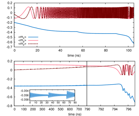
Figure 6: (Color online) Comparison of the current driven dynamics of the spatially averaged magnetization, $\langle\vec{m}\rangle$, for $\theta_{\mathrm{P}}=0^{\circ}$ (top) and $\theta_{\mathrm{P}}=20^{\circ}$ (bottom). The inset in the bottom plot shows the oscillatory motion of the DW induced by the pinning in the barrier. The discontinuities in $\langle m_{x}\rangle$ correspond to changes in the applied current density (see Fig. 7) following the procedure described in the text. Two different scales are used for the time axis of the bottom plot in order to give clear information on the dynamics during the two different phases of the switching process. Note that the dynamics of the preliminary relaxations is omitted in these figures.

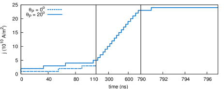
Figure 7: (Color online) The applied current density for the two simulations of Fig. 6 and Fig. 8. The vertical lines in the plot mark a change in the scale of the time axis.

Fig. 6 shows the time evolution of the components of the spatially averaged magnetization, $\langle\vec{m}\rangle$, during the simulations for $\theta_{\mathrm{P}}=0^{\circ}$ (top) and $\theta_{\mathrm{P}}=20^{\circ}$ (bottom). When $\theta_{\mathrm{P}}=0^{\circ}$, the DW rotates around the nanowire axis, as shown by the $y$ and $z$ components of $\langle\vec{m}\rangle$. At the same time, the $x$ component shows that the DW gradually compresses against the barrier as the current density, $j$, is increased from the value $10^{10}\,\mathrm{A/m^{2}}$, to $2\times 10^{10}\,\mathrm{A/m^{2}}$ and $3\times 10^{10}\,\mathrm{A/m^{2}}$ at times $0\,\mathrm{ns}$, $54.9\,\mathrm{ns}$ and $89.4\,\mathrm{ns}$, respectively (dashed line in Fig. 7). The effect of the spin transfer torque is constantly accumulating in time and is stored in form of barrier penetration and DW compression.

In the case $\theta_{\mathrm{P}}=20^{\circ}$, the potential barrier pins the magnetization out of the direction of the nanowire axis, thus breaking the rotational symmetry of the system (i.e. the energy of the system is not invariant for rotations of the magnetization). As a consequence, the DW cannot freely rotate around the axis of the nanowire, but rather precesses narrowly around its equilibrium configuration. The inset at the bottom of Fig. 6 confirms that $\langle m_{x}\rangle$ oscillates weakly and does not vary significantly during the application of increasing current densities (solid line in Fig. 7). Only at time $791.0\,\mathrm{ns}$, when the current density reaches the critical value, $j_{\mathrm{crit}}=24\times 10^{10}\,\mathrm{A/m^{2}}$, the DW starts to penetrate significantly into the barrier. In then takes about $2\,\mathrm{ns}$ for the DW to pass completely through it.

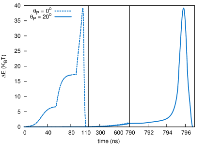
Figure 8: (Color online) Evolution of the energy for the two cases $\theta_{\mathrm{P}}=0^{\circ}$ (dashed line) and $\theta_{\mathrm{P}}=20^{\circ}$ (solid line) considered in Fig. 6 and 7. Units of $k_{\mathrm{B}}T=4.14\times 10^{-21}\,\mathrm{J}$ ($T=300\,K$) are used for the energy. The time axis uses different scales as in Fig. 7.

Fig. 8 shows the micromagnetic energy, $\Delta E$, in the two cases $\theta_{\mathrm{P}}=0^{\circ}$ (dashed line) and $\theta_{\mathrm{P}}=20^{\circ}$ (solid line). $\Delta E(t)$ is computed as $E(t)-E(0)$, where $E(t)$ is the energy of the system at time $t$. The height of the energy barrier, $\Delta E_{\mathrm{max}}$, is almost the same in the two cases. In particular, for $\theta_{\mathrm{P}}=0^{\circ}$, $\Delta E_{\mathrm{max}}=39.24\,k_{\mathrm{B}}T$ while for $\theta_{\mathrm{P}}=20^{\circ}$, $\Delta E_{\mathrm{max}}=39.16\,k_{\mathrm{B}}T$. It is interesting to notice that in the case of a rotationally symmetric barrier, the energy increases gradually as a response to the increase of current density. On the contrary, in the case of an asymmetric barrier, the energy changes very weakly with $j$. In particular, the energy changes less than $1.2\,k_{\mathrm{B}}T$ when $j$ is increased from $10^{10}\,\mathrm{A/m^{2}}$ to $23\times 10^{10}\,\mathrm{A/m^{2}}$. At time $t=791\,\mathrm{ns}$, however, the current is increased to the value $j_{\mathrm{crit}}=24\times 10^{10}\,\mathrm{A/m^{2}}$ and it takes only $5\,\mathrm{ns}$ for the DW to pass through the remaining part of the barrier.

V Discussion

To understand why the rotationally symmetric barrier can be penetrated much more easily than the asymmetric one, we start from Eq. (1). We express the equation in the form where the time derivative of $\vec{m}$ appears only on the left hand side (this requires a substitution of the equation in itself) and both of its sides have been divided by $\gamma M_{\mathrm{s}}$:

$$\frac{1}{\gamma^{\prime}}\partial_{t}\vec{m} = -\vec{m}\times\vec{H}-\alpha\,\vec{m}\times(\vec{m}\times\vec{H})$$ (6)

$${}+(1+\alpha\xi)\,\frac{v}{\gamma}\,\partial_{x}\vec{m}$$

$${}-(\xi-\alpha)\,\frac{v}{\gamma}\,\vec{m}\times\partial_{x}\vec{m},$$

where $\gamma^{\prime}=\gamma/(1+\alpha^{2})$ and $\vec{m}=\vec{M}/M_{\mathrm{s}}$ is a unit vector. The right hand side of this equation receives the contributions of four terms. They are, respectively, the precession term, the damping term, the adiabatic Spin Transfer Torque (STT) and the non-adiabatic STT. The strongest of these terms is typically the precession term, which receives contributions of the order of $10^{6}\,\mathrm{A/m}$ (from the applied field, the demagnetizing field, the magneto-crystalline anisotropy) or higher (from the exchange field). The damping term has lower magnitude, due to the prefactor $\alpha$. For Permalloy, $\alpha\approx 0.01$ and the damping term is then 100 times weaker than the precession term. Despite this, the damping term has a very important role for the physics of the system and has substantial impact on its dynamics. The damping is very effective because it keeps changing the magnetization towards the direction that yields the highest reduction in energy. Its effect, hence, accumulates in time and brings the system to a local energy minimum.

On the other hand, the first STT term (the second STT term is smaller of a factor $\xi-\alpha$ and will be neglected in this analysis) does not have this property: while it can have magnitude similar to the damping term (for Permalloy and $j=10^{12}\,\mathrm{A/m^{2}}$, the adiabatic term can bring contributions of the order of $10^{4}\,\mathrm{A/m}$ in Eq. (6)), it does not always point in the direction which is best suited to pump energy into the system. Often, this term acts in the direction opposite to the much stronger precession term, with the result that the STT pumps energy in and out in an alternate fashion, i.e. there is no “accumulation” of the effect.

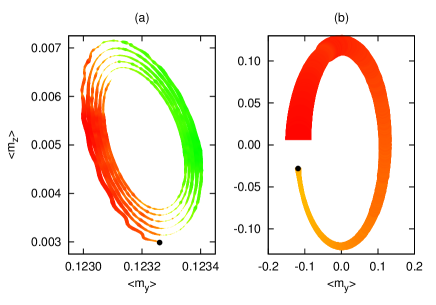
Figure 9: (Color online) Current driven trajectories of the average magnetization, $\langle\vec{m}\rangle$, projected on the $yz$-plane (orthogonal to the nanowire axis). The dynamics is in response to the application of a current density $j=2\times 10^{10}\,\mathrm{A/m^{2}}$ in the case of asymmetric barrier, $\theta_{\mathrm{P}}=20^{\circ}$ (a) and symmetric barrier, $\theta_{\mathrm{P}}=0^{\circ}$ (b). The line thickness is proportional to the magnitude of the energy which is being pumped in (red in color, dark in greyscale) or out (green in color, light in greyscale) at the considered point. The two black dots indicate where the trajectories begin. Note that side (a) shows a few precessions of $\langle m_{x}\rangle$, while side (b) shows only one precession. This is just to avoid the overlapping of the line.

Fig. 9(a) provides an example of this phenomenon. The plot shows the initial part of the trajectory of the spatially averaged normalized magnetization $\langle\vec{m}\rangle=\langle\vec{M}/M_{\mathrm{s}}\rangle$ in the plane $yz$ for the case $\theta_{\mathrm{P}}=20^{\circ}$ of Fig. 6. The points of the trajectory where the energy of the system is increasing, $\partial_{t}E>0$, are coloured in red; the points where it is decreasing, $\partial_{t}E<0$, are coloured in green. The line thickness is proportional to $|\partial_{t}E|$: a thick red line corresponds to maximum energy increase, while a thick green line to maximum energy decrease. The plot shows that once the current is applied, the energy starts increasing while the magnetization moves in the negative $y$ direction. At this point, however, the pinning is strong enough to oppose the current-driven dynamics and pulls the magnetization back, giving rise to a motion spiralling towards a new equilibrium configuration. During the precession, the STT pumps energy in and out, in an alternate fashion. Overall, the current produces changes in $\vec{m}$ of the order of $4\times 10^{-4}$ radians.

A completely different situation is shown in Fig. 9(b), which shows again the dynamics of $\langle\vec{m}\rangle$, but for a DW moving through the rotationally symmetric barrier (case $\theta_{\mathrm{P}}=0^{\circ}$ in Fig. 6). The plot shows that the energy is always pumped in (and never pumped out). Moreover, the rate with which this happens (line thickness) increases in time. This is due to the compression of the DW, which causes a stronger STT effect (higher values of $\partial_{x}\vec{m}$ in Eq. (6)).

The analysis we have carried out demonstrates that it is of fundamental importance to find systems and situations which allow the STT to coherently pump energy into the system. The effectiveness of the STT in the case of rotationally symmetric and asymmetric barriers depends on whether or not the STT points along the optimal direction for energy pumping (i.e. opposite to the damping).

VI Energy barrier

It may be useful at this point to give a more quantitative indication on the height of the barriers which can be penetrated thanks to the mechanism described in this paper. In particular, we would like to find out, given a rotationally symmetric barrier with a given height $\Delta E$, what the required critical current density is in order for the DW to pass through it.

We perform simulations similar to the ones described previously, but here we fix $\theta_{\mathrm{P}}=0^{\circ}$ and change the value for the pinning anisotropy $K_{1}$ from $0.1\times 10^{6}\,\mathrm{J/m^{3}}$ to $1.1\times 10^{6}\,\mathrm{J/m^{3}}$ in steps of $0.1\times 10^{6}\,\mathrm{J/m^{3}}$. For every simulation we also calculate the energy height $\Delta E$ as the difference $\Delta E=E_{\mathrm{max}}-E(0)$, where $E(0)$ is the energy of the system at the beginning of the simulation, while $E_{\mathrm{max}}$ is the maximum value reached throughout the simulation. The values of the critical current, $j_{\mathrm{crit}}$, are plotted in Fig. 10 as function of the barrier height, $\Delta E$.

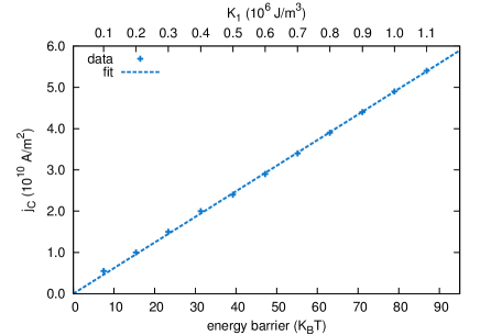
Figure 10: (Color online) Study of the critical current, $j_{\mathrm{crit}}$ required to push the DW through a rotationally symmetric barrier, as a function of the barrier height ($\Delta E$). The top $x$ axis shows the values of the anisotropy constant $K_{1}$ corresponding to the values of $\Delta E$ shown on the bottom axis.

The corresponding values for $K_{1}$ are also shown at the top of the plot. We note that there is a linear relationship between all the three quantities involved: $j_{\mathrm{crit}}$, $\Delta E$ and $K_{1}$. In particular, $\Delta E$ and $K_{1}$ (bottom and top $x$ axis) are linearly proportional and follow the relation $\Delta E(K_{1})=V\,K_{1}$ where $V$ is a parameter with dimensions of a volume and $V=(326.4\pm 0.4)\,\mathrm{nm^{3}}$ (from a least squares fit). This means that — as one may expect — a doubled value for $K_{1}$ corresponds to twice-as-high energy barrier, $\Delta E$.

The linear relation between $j_{\mathrm{crit}}$ and $\Delta E$ is somewhat more difficult to understand intuitively. Fig. 10 shows, however, that the data can be well fitted (see dashed curve) against the function,

$$j_{\mathrm{crit}}(\Delta E)=\tilde{B}\,\Delta E.$$ (7)

In particular, we get $\tilde{B}=(1.498\pm 0.006)\times 10^{29}\,\mathrm{A/(m^{2}J)}$. Or — in terms of thermal energy — it is necessary to apply a fully polarized current density $j=Pj_{\mathrm{app}}$ of $2.48\times 10^{10}\,\mathrm{A/m^{2}}$ in order to push the DW through a potential barrier with height $40\,k_{\mathrm{B}}T$. Assuming a spin polarization $P=0.4$, we find $j_{\mathrm{app}}=6.20\times 10^{10}\,\mathrm{A/m^{2}}$.

We now multiply both sides of equation (7) by the cross sectional area of the nanowire, $\pi R^{2}$:

$$I_{\mathrm{crit}}(\Delta E)=B\,\Delta E,$$ (8)

which relates the critical current $I_{\mathrm{crit}}=\pi R^{2}\,j_{\mathrm{crit}}$ to $\Delta E$. We have $B=\pi R^{2}\,\tilde{B}=(1.177\pm 0.005)\times 10^{13}\,\mathrm{A/J}$.

VII Analytical considerations

In this section we derive a simple analytical model with the aim of understanding the linear proportionality between the current density, $j_{\mathrm{crit}}$, required to push a DW through a potential barrier, and the barrier height, $\Delta E$ (as seen in Fig. 10). We start from the analytical model developed in Ref. Franchin2008prb, (the analytical derivation below is heavily based on this previous work). In particular, we consider the situation where the pinning potential is infinitely high and the DW does not penetrate into the barrier, but rather compresses against it, thus accumulating a certain amount of exchange/compression energy. It is reasonable to expect that if the applied current can accumulate an amount of “compression energy”, $\Delta E$, in the case of an infinite barrier, then it may also be able to push the DW through a finite energy barrier of the same height. We stress that in this context we are just trying to get to a qualitative understanding of the phenomenon, rather than a quantitative analytical model.

First, we write down the energy of the DW, using the one dimensional model, the coordinate system and nomenclature of Ref. Franchin2008prb, ,

$$U=A\int_{0}^{L}\left[(\partial_{x}\theta)^{2}+\sin^{2}\theta\,(\partial_{x}\phi)^{2}\right]\mathrm{d}x.$$

$U$ has the units of energy per cross-sectional area. $A$ is the exchange coupling constant, $L$ the DW width, $\theta$ and $\phi$ are spherical coordinates for the magnetization. In this expression, we consider only the exchange energy and neglect the contribution of the magnetostatic field. The term $\partial_{x}\phi$ is usually smallerFranchin2008prb than $\partial_{x}\theta$, and we neglect it:

$$U=\frac{A}{L}\int_{0}^{1}(\partial_{u}\theta)^{2}\,\mathrm{d}u=-\frac{A}{L}\int_{0}^{\pi}\partial_{u}\theta\,\mathrm{d}\theta,$$

where we also changed the variable of integration twice, from $x$ to $u=x/L$ and from $u$ to $\theta$. In the high current regimeFranchin2008prb , $\partial_{u}\theta=-\frac{3V}{\alpha}\,\sin\frac{\theta}{2}$, and,

$$U=\frac{3AV}{L\alpha}\int_{0}^{\pi}\sin\frac{\theta}{2}\,\mathrm{d}\theta=\frac{6AV}{L\alpha}.$$

Since, $V=\frac{L}{\gamma C}\,v$, we have:

$$U=\frac{6AV}{L\alpha}=\frac{3\mu_{0}M_{\mathrm{s}}}{\gamma\alpha}\,v=\frac{3\mu_{0}\mu_{B}}{e}\,\frac{j}{\gamma\alpha}$$ (9)

For the low current regime the DW deformation is negligible and we get the energy of a relaxed transverse wall of length $L$, $U_{0}=A\pi^{2}/L$. In summary, the present analysis is valid only in the high current regime, i.e. for currents

$$j=Pj_{\mathrm{app}}\gg j_{0}=\frac{2e\gamma}{\mu_{0}\mu_{B}}\,\frac{\alpha A}{L}.$$

In this regime, the DW compresses accumulating an exchange energy $U$ per unit of cross sectional area,

$$U=\frac{6}{\pi^{2}}U_{0}\,\frac{j}{j_{0}},\quad\mathrm{for}\,j\gg j_{0}.$$

The energy pumped in by the current is $\Delta U=U-U_{0}$,

$$\Delta U=U_{0}\left(\frac{6}{\pi^{2}}\,\frac{j}{j_{0}}-1\right),\quad\mathrm{for}\,j\gg j_{0}.$$ (10)

In our system we have $j_{0}=0.026\times 10^{12}\,\mathrm{A}/\mathrm{m}^{2}$ (we have assumed a DW length $L=30\,\mathrm{nm}$). We expect Eq. (10) to hold only when the current exceeds this value. When $j\sim j_{0}$, on the other hand, we may still have important STT effects, but getting to an analytical expression would require to solve exactly the system of equations (14) in Ref. Franchin2008prb, . We can now compare the value obtained for $B$ (see Eq. (8)) from the fit, $B=(1.177\pm 0.005)\times 10^{13}\,\mathrm{A/J}$, with $B=1.013\times 10^{13}\,\mathrm{A/J}$, as obtained from the equation below (derived from Eq. (9)),

$$B=\frac{e\gamma\alpha}{3\mu_{0}\mu_{B}}.$$

Note that $B$ does not depend on the considered geometry, meaning that the total depinning current, $I_{\mathrm{crit}}$, does not depend on the size of the nanowire. In larger nanowires then lower current densities can be used to overcome barriers of the same height in energy. For example, the current density, $j_{\mathrm{app}}=6.20\times 10^{10}\,\mathrm{A/m^{2}}$, required to push a transverse domain wall through a barrier of $40\,k_{\mathrm{B}}T$ in a nanowire with diameter $10\,\mathrm{nm}$, should be reduced by a factor $9$ in nanowires with diameter $30\,\mathrm{nm}$. The optimization of the system geometry necessary to achieve lower current densities and lower switching times are left to future investigations.

In summary, Eq. (10) shows that the amount of exchange energy the DW accumulates by compressing against the infinite potential barrier is proportional to the applied current density. Fig. 10 is then easily understood, assuming the linear behaviour is maintained in the case of finite barrier.

VIII Summary

We have studied a transverse DW in a cylindrical nanowire and its motion through a barrier, modeled as a pinning potential on the magnetization. We determined the critical fields and current densities required to push the DW through the barrier for various directions of the pinning potential. We found that the critical applied field decreases as the pinning direction gets orthogonal to the nanowire axis. On the contrary, the critical current density increases by more than a factor 130 when the pinning direction gets orthogonal to the nanowire axis, meaning that the DW can penetrate the barrier much more easily when the pinning potential is aligned along the axis of the wire, rather than being orthogonal to it.

This study gives further insights into the extraordinary properties of transverse DWs in cylindrical nanowires and motivates experimental investigations on these systems.

- (1) S. S. P. Parkin, M. Hayashi, and L. Thomas, Science 320, 190 (2008)
- (2) G. Tatara and H. Kohno, Phys. Rev. Lett. 92, 086601 (2004)
- (3) M. Kläui, P.-O. Jubert, R. Allenspach, A. Bischof, J. A. C. Bland, G. Faini, U. Rüdiger, C. A. F. Vaz, L. Vila, and C. Vouille, Phys. Rev. Lett. 95, 026601 (2005)
- (4) M. Yan, A. Kákay, S. Gliga, and R. Hertel, Phys. Rev. Lett. 104, 057201 (2010)
- (5) R. Wieser, E. Y. Vedmedenko, P. Weinberger, and R. Wiesendanger, Phys. Rev. B 82, 144430 (2010)
- (6) M. Franchin, G. Bordignon, T. Fischbacher, G. Meier, J. P. Zimmermann, P. de Groot, and H. Fangohr, J. Appl. Phys. 103, 07A504 (2008)
- (7) M. Franchin, T. Fischbacher, G. Bordignon, P. de Groot, and H. Fangohr, Phys. Rev. B 78, 054447 (2008)
- (8) T. Ono and Y. Nakatani, Applied Physics Express 1, 061301 (2008), http://apex.jsap.jp/link?APEX/1/061301/
- (9) J. He and S. Zhang, Applied Physics Letters 90, 142508 (2007), http://link.aip.org/link/?APL/90/142508/1
- (10) K. Matsushita, J. Sato, and H. Imamura, Journal of Applied Physics 105, 07D525 (2009), http://link.aip.org/link/?JAP/105/07D525/1
- (11) A. Bisig, L. Heyne, O. Boulle, and M. Klaui, Applied Physics Letters 95, 162504 (2009), http://link.aip.org/link/?APL/95/162504/1
- (12) G. Finocchio, N. Maugeri, L. Torres, and B. Azzerboni, Magnetics, IEEE Transactions on 46, 1523 (2010), ISSN 0018-9464
- (13) M. Doi, H. Endo, K. Shirafuji, S. Kawasaki, M. Sahashi, H. N. Fuke, H. Iwasaki, and H. Imamura, Journal of Physics D: Applied Physics 44, 092001 (2011), http://stacks.iop.org/0022-3727/44/i=9/a=092001
- (14) R. Wieser, U. Nowak, and K. D. Usadel, Phys. Rev. B 69, 064401 (Feb 2004)
- (15) A. Cao, X. Zhang, J. Wei, Y. Li, C. Xu, J. Liang, D. Wu, and B. Wei, The Journal of Physical Chemistry B 105, 11937 (2001), http://pubs.acs.org/doi/pdf/10.1021/jp0127521, http://pubs.acs.org/doi/abs/10.1021/jp0127521
- (16) R. Lv, A. Cao, F. Kang, W. Wang, J. Wei, J. Gu, K. Wang, and D. Wu, The Journal of Physical Chemistry C 111, 11475 (2007), http://pubs.acs.org/doi/pdf/10.1021/jp0730803, http://pubs.acs.org/doi/abs/10.1021/jp0730803
- (17) K. Pitzschel, J. Bachmann, S. Martens, J. M. Montero-Moreno, J. Kimling, G. Meier, J. Escrig, K. Nielsch, and D. Görlitz, Journal of Applied Physics 109, 033907 (2011), http://link.aip.org/link/?JAP/109/033907/1
- (18) S. Zhang and Z. Li, Phys. Rev. Lett. 93, 127204 (2004)
- (19) T. Fischbacher, M. Franchin, G. Bordignon, and H. Fangohr, IEEE Transactions on Magnetics 43, 2896 (2007)
- (20) Nmag — a micromagnetic simulation environment (2007), http://nmag.soton.ac.uk/
- (21) By definition, is pointing opposite to the functional derivative of the micromagnetic energy, , and hence towards the direction which minimizes . From Eq. (6\@@italiccorr), the damping term is , which is minus the component which would change the magnitude of the magnetization. In other words, the damping term points towards the direction which yields the largest reduction in energy, subject to the constraint .