Phase behaviour of binary mixtures of diamagnetic colloidal platelets in an external magnetic field

Abstract

Using fundamental measure density functional theory we investigate paranematic-nematic and nematic-nematic phase coexistence in binary mixtures of circular platelets with vanishing thicknesses. An external magnetic field induces uniaxial alignment and acts on the platelets with a strength that is taken to scale with the platelet area. At particle diameter ratio $\lambda=1.5$ the system displays paranematic-nematic coexistence. For $\lambda=2$, demixing into two nematic states with different compositions also occurs, between an upper critical point and a paranematic-nematic-nematic triple point. Increasing the field strength leads to shrinking of the coexistence regions. At high enough field strength a closed loop of immiscibility is induced and phase coexistence vanishes at a double critical point above which the system is homogeneously nematic. For $\lambda=2.5$, besides paranematic-nematic coexistence, there is nematic-nematic coexistence which persists and hence does not end in a critical point. The partial orientational order parameters along the binodals vary strongly with composition and connect smoothly for each species when closed loops of immiscibility are present in the corresponding phase diagram.

I Introduction

Dispersions of colloidal plateletlike particles, such as gibbsite vanderbeek04 ; vanderbeek05 , montmorillonite pizzey.c:2004.a ; connolly.j:2007.a or iron-rich beidellite michot.lj2006.a ; paineau.e:2009.a , are susceptible to the influence of magnetic fields, since the particles possess nonvanishing diamagnetic anisotropy. When a magnetic field is applied to an initially isotropic (I) platelet dispersion, the field induces orientational order in the system, thus breaking the rotational symmetry; an orientationally ordered paranematic (P) phase results. The paranematic phase has interesting optical properties, similar to those of the nematic (N) phase. When observed through crossed polarisers, samples of gibbsite suspensions have been shown to exhibit field-induced birefringence vanderbeek.d:2006.a . Birefringence gradients have also been theoretically modelled for a simple model system reich.h:2010.a . The effects of a magnetic field on montmorillonite platelets were studied in Ref. connolly.j:2007.a and on hematite platelets in Ref. ozaki.m:1990.a . Unlike the gibbsite platelets, hematite platelets are ferromagnetic and an I-N transition was not observed; rather the authors found a clustering effect whereby chains of particles were formed due to the platelet-platelet interactions. Such clustering has also been observed in simulations satoh.a:2009.a . Experimental investigations of gibbsite platelets, whereby the suspensions were exposed to magnetic fields vanderbeek.d:2006.a ; vanderbeek.d:2008.a , showed that a paranematic phase occurs in these systems.

The phase behaviour of rods in external aligning fields is well-studied, see e.g. khokhlov.ar:1982.a ; palffymuhoray.p:1982.a ; fraden.s:1993.a ; varga.s:1998.a ; tang.jx:1993.a ; graf.h:1999.a for studies of one-component systems. In Ref. khokhlov.ar:1982.a the effect of external fields on the phase behaviour of rigid rods, freely jointed rods and semiflexible rods was analysed with Onsager theory onsager.l:1949.a : the P-N transition was found to terminate at a critical point in all three cases at a high enough field strength. In Ref. palffymuhoray.p:1982.a the theories of Landau and de Gennes degennes and of Maier and Saupe maier.w:1959.a were used to analyse the effects of an applied field in the nematic phase. The magnetic field-induced birefringence in solutions of tobacco mosaic virus (TMV) particles was studied in Ref. fraden.s:1993.a both experimentally and theoretically (using extensions of Onsager theory). In Ref. varga.s:1998.a the phase behaviour of monodispese rods with varying aspect ratio was studied using the Parsons-Lee scaling parsons.jd:1979.a ; lee.sd:1987.a of the Onsager functional. It was found that the bifurcation density decreases with increasing field strength. The nematic order of model goethite nanorods in a magnetic field was investigated in Ref. wensink_goethite , also using Parsons-Lee theory. The goethite rods were modelled as charged spherocylinders with a permanent magnetic moment along the long axis of the rods. This encourages the rods to align parallel to the field at low field strengths. However, goethite rods possess a negative diamagnetic susceptibility which leads to alignment perpendicular to the field at higher field strengths. These competing effects were found to yield rich phase diagrams including biaxial arrangements of the particles. The phase separation in suspensions of semiflexible fd-virus particles was studied in Ref. tang.jx:1993.a , where a P-N phase transition was found. Effects of an external field on the isotropic, nematic and smectic-A phases of spherocylinders were compared with simulations and theory in Ref. graf.h:1999.a , with results from both approaches being in good agreement.

Even when neglecting positionally ordered phases (such as columnar and crystal phases), the bulk phase behaviour of binary mixtures of non-spherical colloidal particles can be very rich, often including isotropic-isotropic (I-I), isotropic-nematic (I-N) and nematic-nematic (N-N) phase coexistence, depending on the value of the size asymmetry parameter of the two species. The asymmetry parameter may quantify the difference in thickness or lengths of the two species. An example are binary mixtures of thick and thin hard rods in an external field varga.s.:2000.a ; matsuda.h:2004.a ; dobra.s:2006.a . A general feature of the phase behaviour of binary mixtures is a widening of the biphasic region on increasing the asymmetry parameter. In a certain range of the size asymmetry there is typically an I-N-N and/or an I-I-N triple point. Coexistence between two nematic states may or may not end in a critical point depending on the system under study and the value of the asymmetry parameter. A well-studied system is the Zwanzig model for binary hard platelets, where the particles are restricted to occupy three mutually perpendicular directions. This was shown to exhibit rich bulk phase diagrams harnau02 ; bier04 ; harnau08 . We recently explored the phase behaviour of binary mixtures of hard platelets with zero thickness and continuous orientations phillips.j:2010.a using fundamental measure theory (FMT).

Platelets can be characterized by a diamagnetic susceptibility tensor that is diagonal in the platelet frame of reference, with components $\chi_{\parallel}$ in the platelet plane and $\chi_{\perp}$ normal to it. The diamagnetic anisotropy $\Delta\chi\equiv\chi_{\parallel}-\chi_{\perp}\neq 0$, in general, and it may be positive or negative depending on the properties of the platelet material. For Gibbsite platelets $\Delta\chi<0$, therefore the platelets tend to align with their normals perpendicular to the direction of the applied field. In order for the platelets to align uniaxially in the presence of the field, the samples were placed on a central stage and rotated in a horizontally applied field. In Ref. reich.h:2010.a , FMT was used to study the effects of an external field on the phase behaviour of monodisperse platelets. It was found that above a critical field strength the P-N coexistence ceases to exist and the system is homogeneously nematic. In Ref. vandenpol.dme:2008.a , van den Pol et. al. have experimentally investigated the general phase behaviour of the boardlike goethite colloidal particles ($\alpha$-FeOOH) in the presence of an external magnetic field. The particles were found to align parallel to a small magnetic field and perpendicular to a large magnetic field; this had already been known since the observations of Lemaire et. al. lemaire.bj:2002.a . This effect is due to the particles having a permanent magnetic moment along their long axis but the magnetic easy axis being the short axis. An exciting prospect is that suspensions of beidellite platelets, which have a disk-like morphology, have recently been shown to undergo an I-N transition michot.lj2006.a and the nematic phase aligns strongly in the presence of an externally applied magnetic or electric field paineau.e:2009.a . These platelets possess a positive diamagnetic susceptibility and, as such, a simpler experimental setup would be required to investigate the P-N transition; the platelets are expected to align with their normals parallel to the magnetic field.

Since Rosenfeld’s pioneering work rosenfeld89 ; rosenfeld94convex ; rosenfeld95convex there has been much interest in the development of FMT for non-spherical particles, see e.g. hansen-goos . In the current investigation we use the FMT of Ref. phillips.j:2010.a , which is the mixtures generalization of the theory proposed in Ref. esztermann06 , to study binary mixtures of diamagnetic platelets in a magnetic field. We consider three different size ratios representative of the different topologies of the bulk phase diagram and the full range of external field strengths. We investigate how the phase behaviour for each of these three size ratios changes on increasing the external field strength, which we take to scale with the platelet area and to induce uniaxial alignment.

This paper is organised as follows. In Sec. II we outline the density functional theory for the model system. The phase diagrams and results for order parameters are presented in Sec. III and we conclude in Sec. IV.

II Theory

II.1 Pair Interactions, Model Parameters and External Orienting Field

We consider a binary mixture of hard circular platelets with vanishing thickness and continuous positional and orientational degrees of freedom. Particles of species 1 and 2 possess radii $R_{1}$ and $R_{2}$, respectively, and we take $R_{2}>R_{1}$. The pair potential $u_{ij}$ between two particles of species $i$ and $j$, where $i,j=1,2$, models hard core exclusion and is hence given by

$${u_{ij}(\bf{r}-\bf{r}^{\prime},\bm{\omega},\bm{\omega}^{\prime})=\begin{cases}\infty&\text{if particles overlap}\\ 0&\text{otherwise, }\end{cases}}$$ (1)

where r and $\textbf{r}^{\prime}$ are the positions of the particle centres and $\bm{\omega}$ and $\bm{\omega}^{\prime}$ are unit vectors indicating the particle orientations (normal to the particle surface). As a control parameter that characterises the radial bidispersity we use the size ratio

$$\lambda=\frac{R_{2}}{R_{1}}>1.$$ (2)

The effect of a magnetic field on the diamagnetic platelets is described by an external potential for each species,

$$V_{\textrm{ext}}^{(i)}(\theta)=\beta^{-1}W_{i}\sin^{2}\theta,\hskip 14.22636pti=1,2,$$ (3)

where $\beta=1/(k_{B}T)$, with $k_{B}$ being the Boltzmann constant and $T$ absolute temperature; $\theta$ is the angle between the platelet orientation $\bm{\omega}$ and the direction of the external field. The strength of the external potential of species $i$ is related to the material and field properties via

$$W_{i}=-\frac{\beta}{4}B^{2}\Delta\chi_{i}$$ (4)

where $B$ is the magnetic flux density (measured in $\textrm{T})$ and $\Delta\chi_{i}=\chi_{\parallel}^{(i)}-\chi_{\perp}^{(i)}$ is the diamagnetic susceptibility anisotropy (with units of JT^-2) of species $i$, with $\chi_{\parallel}^{(i)}$ and $\chi_{\perp}^{(i)}$ being the susceptibilities perpendicular and parallel to the field, respectively . In general both $W_{1}$ and $W_{2}$ constitute further control parameters. We restrict ourselves in the following to special cases and assume that $W_{i}$ scales with the platelet area, i.e. $W_{i}\sim R_{i}^{2}$. This implies the relationship $W_{2}=\lambda^{2}W_{1}$, and we hence take $W_{1}$ to be our second control parameter, besides the size ratio $\lambda$ itself. Scaling with the platelet area is motivated by the assumption that the platelets interact with an external field in a manner proportional to their mass (neglecting any effects of thickness). We could well envisage that scaling the strength of the potential e.g. with the radius would be another, different yet sensible, choice. We neglect platelet-platelet interactions due to induced dipoles because of their small magnitude, see e.g. the discussion in Ref. reich.h:2010.a .

The thermodynamic state is characterised by two dimensionless densities $c_{1}=\rho_{1}R_{1}^{3}$ and $c_{2}=\rho_{2}R_{1}^{3}$, where $\rho_{1}$ and $\rho_{2}$ are the number densities of the two species, $\rho_{i}=N_{i}/V$, where $N_{i}$ is the number of particles of species $i=1,2$ and $V$ is the system volume. The composition (mole fraction) of the (larger) species 2 is $x=\rho_{2}/(\rho_{1}+\rho_{2})$ and the total dimensionless concentration is $c=(\rho_{1}+\rho_{2})R_{1}^{3}=c_{1}+c_{2}$.

II.2 Density Functional Theory

Density functional theory (DFT) is formulated on the level of the one-body density distributions $\rho_{i}(\bf{r},\bm{\omega})$ of each species $i$. The variational principle evans.r:1979.a asserts that minimising the grand potential functional $\Omega$ yields the true equilibrium density profile,

$$\frac{\delta\Omega([\rho_{1},\rho_{2}],\mu_{1},\mu_{2},V,T)}{\delta\rho_{i}(\textbf{r},\bm{\omega})}=0,\hskip 14.22636pti=1,2$$ (5)

where $\mu_{i}$ is the chemical potential of species $i$. The grand potential functional is given by

$$\Omega([\rho_{1}, \rho_{2}],\mu_{1},\mu_{2},V,T)=F_{\textrm{id}}([\rho_{1},\rho_{2}],V,T)$$

$$+F_{\textrm{exc}}([\rho_{1},\rho_{2}],V,T)+\sum_{i=1}^{2}\int d\textbf{r}\int d\bm{\omega}\rho_{i}(V_{\textrm{ext}}^{(i)}(\textbf{r},\bm{\omega})-\mu_{i}),$$ (6)

where the spatial integral (over r) is over the system volume $V$ and the angular integral (over $\bm{\omega}$) is over the unit sphere. The inter-particle interactions are described by the excess (over ideal gas) contribution to the Helmholtz free energy, $F_{\textrm{exc}}([\rho_{1},\rho_{2}],V,T)$. We skip the explicit definition of the FMT approximation here; this can be found in Ref. phillips.j:2010.a . The free energy functional for a binary ideal gas of uniaxial rotators is given by

$$\beta F_{\textrm{id}}([\rho_{1},\rho_{2}],V,T)=\sum_{i=1}^{2} \int{d\textbf{r}}\int d\bm{\omega}\rho_{i}(\textbf{r},\bm{\omega})$$

$$\times[\ln(\rho_{i}(\textbf{r},\bm{\omega})\Lambda_{i}^{3})-1],$$ (7)

where $\Lambda_{i}$ is the (irrelevant) thermal wavelength of species $i$.

For bulk fluid states (i.e. with the density distribution not depending on r) the orientational distribution functions (ODFs), $\Psi_{i}(\theta)$, $i=1,2$, are related to the one-body density distributions by $\rho_{i}(\textbf{r},\bm{\omega})=\rho_{i}\Psi_{i}(\theta)$. There is no dependence of the ODF on the azimuthal angle $\phi$ since the platelets are uniaxial rotators, and we assume that only uniaxial states are formed. A powerful feature of DFT is that $V_{\textrm{ext}}^{(i)}(\textbf{r},\bm{\omega})$ (3) appears explicitly in the grand potential and therefore enters straightforwardly into the minimisation procedure (5); see the appendix for the explicit form of the corresponding Euler-Lagrange equations that we solve numerically.

The requirements for phase coexistence between two phases A and B are the mechanical and chemical equilibria between the two phases and the equality of temperature in the two coexisting phases (which is trivial in hard-body systems). Hence we have the non-trivial conditions: the equality of pressure $p^{A}=p^{B}$ and the equality of chemical potentials $\mu_{i}^{A}=\mu_{i}^{B}$, where $i=1,2$ again labels the species, and $A,B$ labels the phase. We calculate the total Helmholtz free energy $F=F_{\textrm{id}}+F_{\textrm{exc}}$ numerically by inserting $\Psi_{i}(\theta)$ into the free energy functional. Likewise, the pressure can be obtained numerically as $p=-F/V+\sum_{i=1}^{2}\rho_{i}\partial(F/V)/\partial\rho_{i}$ and the chemical potentials as $\mu_{i}=\partial(F/V)/\partial\rho_{i}$. We define a reduced pressure $p^{*}=\beta pR_{1}^{3}$ and reduced chemical potentials $\mu_{i}^{*}=\beta\mu_{i}$. The equations for phase coexistence are three equations for four unknowns (two statepoints each characterised by two densities) hence regions of two-phase coexistence depend parametrically on one free parameter (which can be chosen arbitrarily, e.g. as the value of composition $x$ in one of the phases) and are solved numerically with a Newton-Raphson procedure press.wh:2007.a . The resulting set of solutions yields the binodal. P-N-N triple points are located where the P-N and N-N coexistence curves cross. In the fieldless case there is, of course, not a paranematic phase, but an isotropic phase.

We characterize orientationally ordered phases (P and N) of the binary mixture by two partial order parameters, $S_{1}$ and $S_{2}$, defined by

$$S_{i}=4\pi\int_{0}^{\pi/2}d\theta\sin(\theta)\Psi_{i}(\theta)P_{2}(\cos\theta),$$ (8)

where $P_{2}(\cos\theta)=(3\cos^{2}\theta-1)/2$ is the second Legendre polynomial in $\cos\theta$.

III Results

We first review the behaviour of the pure system under the influence of an aligning field reich.h:2010.a . The inset of Fig. 1(a) shows the phase diagram for a system composed of particles of species 1 only. Upon increasing the field strength $W_{1}$, the coexisting concentrations $c_{1}$ initially shift to lower values. The biphasic density gap decreases slightly as the strength of the external potential is increased. At approximately $W_{1}=0.02$, the paranematic coexistence concentration starts to increase, while the nematic coexistence concentration continues to decrease. The two branches of the binodal meet at a critical point at $c_{1}^{\textrm{crit}}=0.42$. For $W_{1}>W_{1}^{\textrm{crit}}=0.045$, there is no longer a phase transition and complete destabilisation of the P-N transition results in a homogeneous nematic phase. For the case of equal sizes of the two components, the pure system of species 2 possesses the same phase diagram, see the binodal for the case $\lambda=1$ in main plot of Fig. 1(a). However, due to the definition of $c_{2}$ (recall that $c_{2}=\rho_{2}R_{1}^{3}$, using the radius of species 1 in order to obtain a dimensionless quantity) and the scaling of $W_{2}$ with the square of the size ratio ($W_{2}=\lambda^{2}W_{1}$), the phase diagram of the pure system of species 2 displays strong variation with size ratio $\lambda$, as shown in Fig. 1(a). A shift to both smaller values of $c_{2}$ and of $W_{1}$ occurs upon increasing the value of $\lambda$. However, this effect is entirely due to the choice of coordinates, which for both pure systems are related via $c_{2}=c_{1}/\lambda^{3}$ and $W_{2}=W_{1}/\lambda^{2}$. Numerical values for the location of the critical point are summarised in Tab. 1.

$\lambda$	$\lambda^{2}$	$\lambda^{3}$	$c_{2}^{\textrm{crit}}$	$W_{1}^{\textrm{crit}}$
1	1	1	0.42	0.045
1.5	2.25	3.375	0.124	0.019
2	4	8	0.053	0.011
2.5	6.25	15.625	0.027	0.0072

Table 1: Scaling of the location of the critical point with size ratio: Critical concentration $c_{2}^{\textrm{crit}}=\lambda^{-3}c^{\textrm{crit}}$ and critical field strength $W_{1}^{\textrm{crit}}=\lambda^{-2}W^{\textrm{crit}}$ for a range of size ratios $\lambda$, where $c^{\textrm{crit}}$ and $W^{\textrm{crit}}$ are the critical concentration and field strength in the pure system (without species index).

The variation of the order parameter $S$ for monodisperse platelets with field strength is displayed in Fig. 1(b). In the field-free case, $W_{1}=0$, the nematic phase at coexistence possesses an unusually small order parameter, see e.g. the discussion in Ref. reich07 . For all size ratios, as $W_{1}$ is increased, the coexistence value of $S$ in the paranematic phase increases monotonically, and the value of $S$ along the nematic branch of the binodal decreases with increasing field strength. This is consistent with the fact that the coexistence density decreases as the field strength increases, overcompensating for the ordering effect caused by the applied field. At the critical point the nematic order parameter takes on the value $S_{2}=0.27$. For increasing values of $\lambda=1,1.5,2$ and $2.5$, the critical point shifts to smaller values of field strengths.

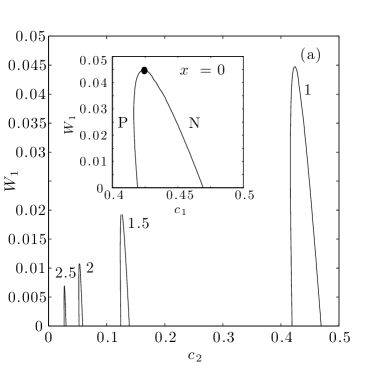
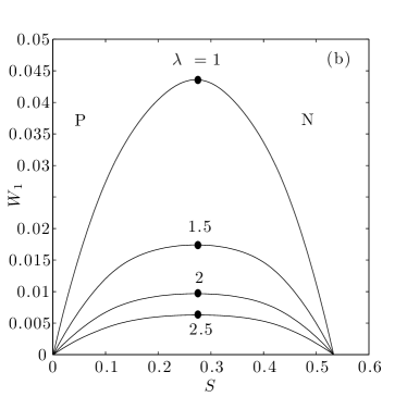
Figure 1: Paranematic-nematic phase diagram of the one-component system(s). (a) Behaviour of the pure system of species 2 (i.e. $x=1$). The variation of the paranematic (P) and nematic (N) coexistence concentrations, $c_{2}$ (horizontal axis) with the strength of the aligning field $W_{1}$ (vertical axis) is shown for $\lambda=1,1.5,2$ and $2.5$ (from right to left, as indicated). The inset shows the phase diagram for the pure system of species 1 (i.e. $x=0$). This is equivalent to the case $\lambda=1$ in the main plot when identifying the horizontal axes. The critical point is depicted as a filled circle. (b) Variation of the orientational order parameter $S=S_{2}$ along the paranematic and nematic branches of the binodal (horizontal axis) of the pure system of species 2, with increasing field strength $W_{1}$ (vertical axis) for the same size ratios as in (a). Critical points are depicted as filled circles.

We next consider the binary mixture in the external field and hence explore the full range of compositions, $0\leq x\leq 1$. In Fig. 2 the phase diagram for $\lambda=1.5$ is shown. We consider a range of external field strengths up to $W_{1}=0.15$ (which corresponds to $W_{2}=\lambda^{2}W_{1}=0.3375$). For the fieldless case, $W_{1}=0$, there is I-N phase coexistence over the entire range of compositions $x$. We display this phase diagram (and subsequent ones) both in the $(c_{1},c_{2})$ representation [Fig. 2(a)] as well as in the $(x,p^{*})$ representation [Fig. 2(b)]. Tie-lines are omitted for clarity; in the $(c_{1},c_{2})$ representation these connect the lower branch of the binodal to the upper branch in such a way that the isotropic (or paranematic) phase is rich in (the smaller) species 1 and the nematic phase is rich in (the larger) species 2. In the $(x,p^{*})$ representation [Fig. 2(b)] the tie lines are (trivially) horizontal due to the condition of equal pressures in the coexisting phases. For $W_{1}=0.01$, the binodal still connects to the axes (which correspond to the pure systems). Recall that the P-N transition still occurs in the pure systems at this field strength, cf. Fig. 1(a). However, the isotropic phase has now become a weakly-ordered paranematic phase. Hence there is P-N phase coexistence over the entire range of compositions. The isotropic phase has been replaced by a paranematic phase, because the order parameter along the lower branch of the binodal is non-zero, see Fig. 2(c) and (d), where the partial nematic order parameters are shown for species 1 and 2, respectively. On increasing $W_{1}$ to $0.03$, the upper and lower branches of the binodal still persist to the pure system of smaller platelets, consistent with the findings of Ref.reich.h:2010.a . However, the binodal does not touch the $c_{2}$-axis, indicating that there is no longer a phase transition in the pure system of species 2 (we found the critical field strength for the monodisperse system at $\lambda=1.5$ to be $0.019$, which is less than $0.03$, Fig. (1a)). Hence the two branches of the binodal connect at a (lower, in pressure) critical point. Therefore the state of the system changes continuously from paranematic to nematic for compositions greater than about 0.7 by increasing the pressure. For compositions less than this value, increasing the pressure from below the lower branch of the binodal to the upper branch of the binodal, the system, as before, passes through a biphasic region. For $W_{1}=0.05$ the departure of the binodal from $c_{1}=0$ (and $x=0$) occurs as is consistent with the critical field strength being $W_{1}^{\textrm{crit}}=0.045$ in the pure system. The result is a phase diagram in which the two branches of the binodal have joined to form a closed loop of immiscibility. There is a larger range of compositions towards the $x=1$ side of the phase diagram (approximately $x>0.45$) than towards the $x=0$ side of the phase diagram (approximately $x<0.02$), where an increase in pressure leads to a continuous change in state from a paranematic state to a nematic state. The order parameter of species 1, measured along the binodal varies with composition [Fig. (2c)] such that for $W_{1}=0,0.01$ and $0.03$ the paranematic and nematic branches of the binodal do not connect on the low-composition side of the order parameter graph since these values of $W_{1}$ are less than $W_{1}^{\textrm{crit}}=0.045$. For $0.05\leq W_{1}\leq 0.15$ the two branches of the binodal connect on the low-composition side of the graph. For $W_{1}=0$ and $0.01$ the two branches of the binodal do not connect on the high-composition side of the graph since these values of $W_{1}$ are smaller than $W_{2}^{\textrm{crit}}=\lambda^{2}W_{1}^{\textrm{crit}}=0.019$. For $W_{1}\geq 0.05$ the partial order parameters measured along the binodal form closed loops. These islands become smaller with increasing field strength and eventually coalesce to a point when the double critical point is reached. The partial order parameters of species 2 [Fig. (2d)] follow a similar pattern except that the order at a given statepoint is higher than that for species 1, as one could expect, given that species 2 is of the larger size.

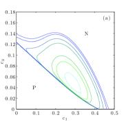
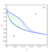
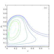
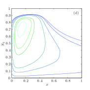
Figure 2: Phase behaviour of binary platelet mixtures with size ratio $\lambda=1.5$ and external potential strength $W_{1}=0,0.01,0.03,0.05,0.07,0.1,0.12$ and $0.15$ (with $W_{2}=\lambda^{2}W_{1}$) from outside to inside. Shown are phase diagrams in (a) the $(c_{1},c_{2})$ representation and (b) in the $(x,p^{*})$ representation. The partial order parameters $S_{i}$ along the binodal are shown in (c) for species 1 and in (d) for species 2.

In Fig. 3 we show results for $\lambda=2$. Increasing the size ratio to this value leads to an increase of the size of the I-N biphasic region phillips.j:2010.a . The fieldless case possesses a reentrant phenomenon whereby the system undergoes the following change of state when increasing the pressure at fixed mole fraction at around $x=0.7$ starting in the isotropic region: I$\rightarrow$I-N$\rightarrow$N$\rightarrow$I-N$\rightarrow$N. In addition, there is N-N coexistence between a nematic phase rich in species 1 (N₁) and a nematic phase rich in species 2 (N₂) ending in an upper critical point and an I-N-N triple point. Applying a small field strength of $W_{1}=0.02$, the binodal no longer reaches the pure system of species 2, as $W_{1}=0.02>W_{1}^{\textrm{crit}}=0.011$, which is the critical field strength for the monodisperse system at $\lambda=2$. An effect of this is that the reentrant part of the phase diagram alters: the range of compositions for which the system undergoes P$\rightarrow$P-N$\rightarrow$N$\rightarrow$P-N$\rightarrow$N at just over $x=0.5$ is much smaller than in the fieldless case. The binodal ends in a tail-like feature at just under $x=0.6$. Aside from these differences, the rest of the phase boundaries follow closely those of the fieldless case, though remaining slightly inside those of the latter. There is N-N coexistence ending in an upper critical point. The triple point is retained as a P-N-N line in the $(x,p^{*})$ representation and a triangle in the $(c_{1},c_{2})$ representation although we do not show these features in the plots for clarity. Upon increasing the field, triple phase coexistence vanishes, i.e. the triple point collapses onto two-phase coexistence. We have not calculated the precise value of the external field where this happens. We expect this value to be different from the values where the binodal detaches from either of the density axes (i.e. differ from the critical field strengths in the pure systems). Applying a field strength $W_{1}=0.6$, which is much greater than the critical field strength for the monodisperse case, $W_{1}^{\textrm{crit}}=0.045$, leads to a closed loop of immiscibility. The nematic phase rich in small platelets (N₂) and the paranematic phase have merged.

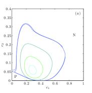
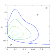
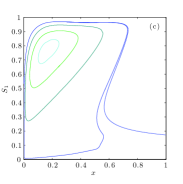
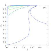
Figure 3: Same as Fig. 2 except for size ratio $\lambda=2$ and for external field strengths $W_{1}=0,0.02,0.6,1$ and $1.2$.

In Fig. 4 we present results for $\lambda=2.5$. The fieldless case displays I-N coexistence, an I-N-N triple point and coexistence between two nematic states, which does not end in a critical point. Applying just a small field $W_{1}=0.01$ has a considerable effect on the phase behaviour: the pure system of species 2 looses the P-N transition as $W_{1}=0.01>W_{1}^{\textrm{crit}}=0.0069$. However, the transition persists in the pure system of species 1. Hence, there is still P-N coexistence and indeed a tail between about $x=0.5$ and $x=0.6$ where reentrant behaviour occurs. For $W_{1}=1$, there is no P-N transition for either of the pure limits. There is, however, a large immiscibitity gap between two distinct nematic phases, $N_{1}$ and $N_{2}$. Increasing the field strength raises the phase coexistence to higher pressures and narrows the phase coexistence region. However, large steps in field strength are required to have a significant effect on the system. $W_{1}=7$ (which corresponds to $W_{2}=49$) is approximately 45 times stronger than the field reqired to homogenise the system at $\lambda=1.5$ and yet even with such a high field strength, there persists a wide coexistence region. The order parameter curves approach very high values (close to 1) for large values of $W_{1}$. This forms a limit to the densities at which we may probe at $\lambda=2.5$: for very high order parameters it is numerically difficult to determine the ODFs, even with very fine $\theta$-grids.

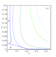
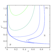
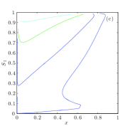
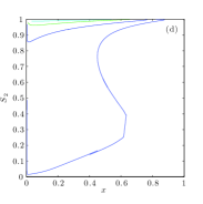
Figure 4: Same as Fig. 2 except for $\lambda=2.5$ and for external field strengths $W_{1}=0,0.01,1,2.5,5$ and $7$. In (c) and (d) we only present partial order parameters for $W_{1}=0.01,1,2.5$ and $5$ for clarity. The small kinks at low values of $S_{i}$ in (c) and (d) are due to numerical artifacts.

IV Conclusions and Outlook

We have investigated the effects of an external aligning (magnetic) field on the phase behaviour of binary mixtures of circular hard core platelets with zero thickness. Using the FMT of Refs. esztermann06 ; phillips.j:2010.a , we have traced paranematic and nematic phase boundaries and have examined the partial nematic order parameters at coexistence. Three different representative values for the radial bidispersity ($\lambda=1.5,2,2.5$) have been studied. The topologies for each of these values are different from each other in the fieldless case. For the smallest size ratio considered, $\lambda=1.5$, the fieldless case shows only I-N phase coexistence over the entire range of compositions. For $\lambda=2$, besides I-N coexistence there is also N-N coexistence ending in an upper critical point and an I-N-N triple point occurs. For $\lambda=2.5$ the N-N phase coexistence does no longer end in a critical point (at least up to the densities we considered). Applying the external field induces paranematic order in the low-density regions of the phase diagrams (which are isotropic in the absence of a field). Increasing the field strength leads in all cases to a narrowing of the biphasic P-N region. The P-N transition further destabilises upon increasing the external field strength. The system becomes more strongly ordered, such that for $\lambda=1.5$ and 2 phase coexistence disappears (at a double critical point) and the system is in a single-phase nematic state for all statepoints. The field strength required to complete the homogenisation increases for increasing size ratio. In contrast, for $\lambda=2.5$, the coexisting nematic states become so well-ordered that the system does not become homogeneously nematic up to the field strengths we have applied.

Results from computer simulation studies for this (or a similar) model mixture are highly desirable, as are experimental studies. Colloidal platelets are often significantly polydisperse in both radius and thickness, see for example Ref. vanderkooij.f.m:2000.a , so effects due to polydispersity will play a role in experimental systems, which are not accounted for in the present theory. Recently, the P-N interface in suspensions of boardlike goethite particles has been investigated experimentally vandenpol.e:prep . Anticipating that similar studies could be made in systems of colloidal platelets, a further exciting avenue would be to investigate the properties of the P-N interface using FMT, which has already been shown to compare well with experimental and simulation results for the I-N interface vanderbeek.d:2006.b . It would be interesting to consider in theoretical work the effects that are induced by finite thickness of the platelets. In the present study we restricted ourselves to mixtures with moderate size asymmetry, as we expect the theory to describe these accurately. Investigating highly asymmetric mixtures, possibly based on the depletion picture, is an interesting issue for future work.

Appendix A Self-Consistency Equations for the Orientational Distribution Functions

We give a summary of the equations that are necessary to find the ODFs at a given composition, $x$ and concetration, $c$. The excess free energy from FMT is the sum of the right hand sides of Eqs. (13) and (27) of Ref. phillips.j:2010.a . Inserting this, together with the ideal free energy (7) and the external potential (3), into the grand potential functional (6), and employing the minimisation principle (5) leads to two coupled Euler-Lagrange equations for the ODFs:

$$\Psi_{1}(\theta) =\frac{1}{Z_{1}}\exp\bigg{[}-8\pi c\int_{0}^{\pi/2}d\theta^{\prime}\sin\theta^{\prime}K(\theta,\theta^{\prime})[(1-x)\Psi_{1}(\theta^{\prime})+\frac{1}{2}x(\lambda^{2}+\lambda)\Psi_{2}(\theta^{\prime})]$$

$$-32\pi c^{2}\int_{0}^{\pi/2}d\theta^{\prime}\sin\theta^{\prime}\int_{0}^{\pi/2}d\theta^{\prime\prime}\sin\theta^{\prime\prime}L(\theta,\theta^{\prime},\theta^{\prime\prime})$$

$$[(1-x)^{2}\Psi_{1}(\theta^{\prime})\Psi_{1}(\theta^{\prime\prime})+2x(1-x)\lambda^{2}\Psi_{1}(\theta^{\prime})\Psi_{2}(\theta^{\prime\prime})+x^{2}\lambda^{4}\Psi_{2}(\theta^{\prime})\Psi_{2}(\theta^{\prime\prime})]+W_{1}\sin^{2}\theta\bigg{]},$$ (9)

$$\Psi_{2}(\theta) =\frac{1}{Z_{2}}\exp\bigg{[}-8\pi c\int_{0}^{\pi/2}d\theta^{\prime}\sin\theta^{\prime}K(\theta,\theta^{\prime})[x\lambda^{3}\Psi_{2}(\theta^{\prime})+\frac{1}{2}(1-x)(\lambda^{2}+\lambda)\Psi_{1}(\theta^{\prime})$$

$$-32\pi c^{2}\int_{0}^{\pi/2}d\theta^{\prime}\sin\theta^{\prime}\int_{0}^{\pi/2}d\theta^{\prime\prime}\sin\theta^{\prime\prime}L(\theta,\theta^{\prime},\theta^{\prime\prime})$$

$$[x^{2}\lambda^{6}\Psi_{2}(\theta^{\prime})\Psi_{2}(\theta^{\prime\prime})+2x(1-x)\lambda^{4}\Psi_{1}(\theta^{\prime})\Psi_{2}(\theta^{\prime\prime})+(1-x)^{2}\lambda^{2}\Psi_{1}(\theta^{\prime})\Psi_{1}(\theta^{\prime\prime})]+W_{2}\sin^{2}\theta\bigg{]},$$ (10)

where the constants $Z_{1}$ and $Z_{2}$ are such that the normalisation $\int d\bm{\omega}\Psi_{i}(\bm{\omega})=1$, for $i=1,2$. The numerical procedure is the same as that described in Ref. phillips.j:2010.a , which is an extension of the procedure introduced in Ref. herzfeld84 . The integral kernel $K(\theta,\theta^{\prime})$ is

$$K(\theta,\theta^{\prime})= \int_{0}^{2\pi}d\phi\sin\gamma=\int_{0}^{2\pi}d\phi\sqrt{1-(\bm{\omega}\cdot\bm{\omega}^{\prime})^{2}}$$

$$=\int_{0}^{2\pi}d\phi\sqrt{1-(\cos\theta\cos\theta^{\prime}+\sin\theta\sin\theta^{\prime}\cos\phi)^{2}},$$ (11)

where $\phi$ is the difference between the azimuthal angles of the two platelets and the kernel $L(\theta,\theta^{\prime},\theta^{\prime\prime})$ is

$$L(\theta,\theta^{\prime},\theta^{\prime\prime})= \int_{0}^{2\pi}\int_{0}^{2\pi}d\phi^{\prime}d\phi^{\prime\prime}|\bm{\omega}\cdot(\bm{\omega}^{\prime}\times\bm{\omega}^{\prime\prime})|$$

$$=\int_{0}^{2\pi}\int_{0}^{2\pi}d\phi^{\prime}d\phi^{\prime\prime}|\sin\theta(\sin\phi^{\prime}\sin\theta^{\prime}\cos\theta^{\prime\prime}$$

$$\hskip 14.22636pt+\cos\theta^{\prime}\sin\phi^{\prime\prime}\sin\theta^{\prime\prime})+\cos\theta(\cos\phi^{\prime}\sin\theta^{\prime}\sin\phi^{\prime\prime}\sin\theta^{\prime\prime}$$

$$\hskip 14.22636pt-\sin\phi^{\prime}\sin\theta^{\prime}\cos\phi^{\prime\prime}\sin\theta^{\prime\prime})|.$$ (12)

The solutions of Eqs. (A) and (A), $\Psi_{1}(\theta)$ and $\Psi_{2}(\theta)$, are then inserted into the equations $p^{\textit{A}}=p^{\textit{B}}$ and $\mu_{i}^{\textit{A}}=\mu_{i}^{\textit{B}}$, $i=1,2$ in order to find the coexisting states. Triple points are located where the P-N binodals and the N-N binodals intersect.

- (1) D. van der Beek, T. Schilling, and H. N. W. Lekkerkerker, J. Chem. Phys. 121, 5423 (2004).
- (2) D. van der Beek, A. V. Petukhov, S. M. Oversteegen, G. J. Vroege, and H. N. W. Lekkerkerker, Eur. Phys. J. E 16, 253 (2005).
- (3) C. Pizzey, S. Klein, E. Leach, J. S. van Duijneveldt, and R. M. Richardson, J. Phys.: Condens. Matter 16, 2479 (2004).
- (4) J. Connolly, J. S. van Duijneveldt, S. Klein, C. Pizzey, and R. M. Richardson, J. Phys.: Condens. Matter 19, 156103 (2007).
- (5) L. J. Michot, I. Bihannic, S. Maddi, S. S. Funari, C. Baravian, P. Levitz, and P. Davidson, Proc. Natl. Acad. Sci. U.S.A. 44, 16101 (2006).
- (6) E. Paineau, K. Antonova, C. Baravian, I. Bihannic, P. Davidson, I. Dozov, M. Impéror-Clerc, P. Levitz, A. Madsen, F. Meneau, and L. J. Michot, J. Phys. Chem. B 113, 15858 (2009).
- (7) D. van der Beek, A. V. Petukhov, P. Davidson, J. Ferré, J. P. Jamet, H. H. Wensink, G. J. Vroege, W. Bras, and H. N. W. Lekkerkerker, Phys. Rev. E 73, 041402 (2006).
- (8) H. Reich and M. Schmidt, J. Chem. Phys. 132, 144509 (2010).
- (9) M. Ozaki, N. Ookoshi, and E. Matijević, J. Coll. Interf. Sci. 137, 546 (1990).
- (10) A. Satoh and Y. Sakuda, Mol. Phys. 107, 1621 (2009).
- (11) D. van der Beek, P. Davidson, H. H. Wensink, G. J. Vroege, and H. N. W. Lekkerkerker, Phys. Rev. E 77, 031708 (2008).
- (12) A. R. Khokhlov and A. N. Semenov, Macromolecules 15, 1272 (1982).
- (13) P. Palffymuhoray and D. A. Dunmur, Phys. Lett. 91, 121 (1982).
- (14) S. Fraden, G. Maret, and D. L. D. Caspar, Phys. Rev. E 48, 2816 (1993).
- (15) S. Varga, G. Jackson, and I. Szalai, Mol. Phys. 93, 377 (1998).
- (16) J. X. Tang and S. Fraden, Phys. Rev. Lett. 71, 3509 (1993).
- (17) H. Graf and H. Löwen, J. Phys.: Condens. Matter 11, 1435 (1999).
- (18) L. Onsager, Ann. N. Y. Acad. Sci. 51, 627 (1949).
- (19) P. G. de Gennes and J. Prost, The physics of liquid crystals, 2nd ed. (Clarendon Press, Oxford, 1995).
- (20) W. Maier and A. Saupe, Z. Naturforsch 14, .
- (21) J. D. Parsons, Phys. Rev. A 19, 1225 (1979).
- (22) S. D. Lee, J. Chem. Phys. 87, 4972 (1987).
- (23) H. H. Wensink and G. J. Vroege, Phys. Rev. E 72, 031708 (2005).
- (24) S. Varga and I. Szalai, Phys. Chem. Chem. Phys. 2, 1955 (2000).
- (25) S. Dobra, I. Szalai, and S. Varga, J. Chem. Phys. 125, 074907 (2006).
- (26) H. Matsuda, T. Koda, A. Nishioka, and S. Ikeda, J. Phys. Soc. Jpn. 73, 2753 (2004).
- (27) L. Harnau and S. Dietrich, Phys. Rev. E 66, 051702 (2002).
- (28) M. Bier, L. Harnau, and S. Dietrich, Phys. Rev. E 69, 021506 (2004).
- (29) L. Harnau, Mol. Phys. 106, 1975 (2008) and references therein.
- (30) J. Phillips and M. Schmidt, Phys. Rev. E 81, 041401 (2010).
- (31) E. van den Pol, D. M. E. Thies-Weesie, A. V. Petukhov, P. Panine, and G. J. Vroege, J. Phys.: Condens. Matter 20, 404219 (2008).
- (32) B. J. Lemaire, P. Davidson, J. Ferré, J. P. Jamet, P. Panine, I. Dozov, and J. P. Jolivet, Phys. Rev. Lett. 88, 125507 (2002).
- (33) Y. Rosenfeld, Phys. Rev. Lett. 63, 980 (1989)
- (34) Y. Rosenfeld, Phys. Rev. E 50, R3318 (1994).
- (35) Y. Rosenfeld, Mol. Phys. 86, 637 (1995).
- (36) H. Hansen-Goos and K. Mecke, Phys. Rev. Lett. 102, 018302 (2008); J. Phys.: Condens. Matter 22, 364107 (2010).
- (37) A. Esztermann, H. Reich, and M. Schmidt, Phys. Rev. E. 73, 011409 (2006).
- (38) R. Evans, Adv. Phys. 28, 143 (1979).
- (39) W. H. Press, S. A. Teukolsky, W. T. Vetterling, and B. P. Flannery, Numerical Recipes, 3rd ed. (Cambridge University Press, Cambridge, 2007).
- (40) H. Reich, M. Dijkstra, R. van Roij, and M. Schmidt, J. Phys. Chem. B 111, 7825 (2007).
- (41) F. M. van der Kooij, K. Kassapidou, and H. N. W. Lekkerkerker, Nature 406, 868 (2000).
- (42) E. van den Pol, A. Lupascu, and G. J. Vroege, unpublished (2010).
- (43) D. van der Beek, H. Reich, P. van der Schoot, M. Dijkstra, T. Schilling, R. Vink, M. Schmidt, R. van Roij, and H. N. W. Lekkerkerker, Phys. Rev. Lett. 97, 087801 (2006).
- (44) J. Herzfeld, A. Berger, and J. Wingate, Macromolecules 17, 1718 (1984).