A Lifting Relation from Macroscopic Variables to Mesoscopic Variables in Lattice Boltzmann Method: Derivation, Numerical Assessments and Coupling Computations Validation

, , ,

Abstract

In this paper, analytic relations between the macroscopic variables and the mesoscopic variables are derived for lattice Boltzmann methods (LBM). The analytic relations are achieved by two different methods for the exchange from velocity fields of finite-type methods to the single particle distribution functions of LBM. The numerical errors of reconstructing the single particle distribution functions and the non-equilibrium distribution function by macroscopic fields are investigated. Results show that their accuracy is better than the existing ones. The proposed reconstruction operator has been used to implement the coupling computations of LBM and macro-numerical methods of FVM. The lid-driven cavity flow is chosen to carry out the coupling computations based on the numerical strategies of domain decomposition methods (DDM). The numerical results show that the proposed lifting relations are accurate and robust.

Key words: LBM, Navier-Stokes equations, non-equilibrium distribution functions, multi-scale perturbation expansion, coupling computation, FVM

1 Introduction

In the past decades, LBM has been widely used to simulate fluid flow problems [1, 2], including complex turbulent fluid flows [3, 4] and multiscale modeling[5, 6]. This method is based on the Boltzmann kinetic equation which is used to describe a number of interacting populations of particles. As described in [7], “The LBE could potentially play a twofold function-as a telescope for the atomistic scale and a microscope for the macroscopic scale”. In [8] dense fluids flow past and through a carbon nano tube (CNT) was studied by a hybrid model coupling LBM and MDS. The authors pointed out that replacing the finite volume solver by a LBM aims to take advantage of the mesoscopic modeling inherent in LB simulations. Thus LBM is a mesoscopic method in nature is a widely-accepted understanding in the literature. The macroscopic parameters such as fluid density, velocity and pressure can be obtained via some averages of the mesoscopic variable which conform the basic conservation laws of mass and momentum [2]. In practical applications of LBM to simulate a macroscopic problem, a crucial problem is confronted, that is, a reasonable initial meso-field must be specified to start the evolution process. The first initializing method was proposed in [9] in 1993. Recently, several methods have been proposed to improve the accuracy of numerical results and reduce the initial layers (oscillation layers) [10, 11]. Such oscillations have a numerical origin and are due to the artificial compressibility of LBM. Here, “ initial layer ” refers to such a computational stage within which the macroscopic parameters are oscillating. When the initial data is not well-prepared, there is an initial layer during which the solution adapts itself to match the profile dictated by the environment. For the LBM, the existence of the initial layers is a common phenomenon [10]. In this paper, we will derive the lifting relations between the macroscopic variables and the mesoscopic variables in LBM by two ways. According to the authors’ knowledge, the proposed lifting relations in this paper are different from those in the existing literature [9, 10, 11, 12, 13, 14, 15]. The proposed relations will offer us some new views about the reconstruction of nonequilibrium distribution functions in LBM.

Challenging multiscale phenomena or processes are widely existed in material science, chemical engineering process, energy and power engineering, and other engineering fields. Generally speaking, for a multiscale problem, we often must use different methods to numerically model the processes at different geometric sub-regions and exchange solution information at interface [16, 17, 18, 19]. Such coupling computations are widely adopted in the present-day multiscale simulation. As indicated above LBM is a kind of mesoscopic methods, which is a candidate to implement the meso-macro or micro-meso coupling computations in engineering applications [7]. So, the proposed method not only can be used to obtain a better initial field for LBM, but also can be adopted in the multi-scale computation. For example in [7] the possibility of coupling LBM with molecular dynamics simulation (MDS) was investigated and found that with proper time and geometric scales the two numerical methods can be coupled. And in [8] such coupling simulation was conducted. In the existing literatures the coupling of finite difference method (FDM, which is a macrosopic method) with LBM was adopted in [19, 20, 21], but the proposed coupling method is similar to a multigrid method and a simple regularization formula is used in their computations. The regularization formula in [19] only considers the first-order approximation of the single particle distribution function and the coupling formula in [20] is only used to deal with the one-dimensional reaction-diffusion system. In [8] the coupling between LBM and MDS was implemented by exchange of velocity and velocity gradient at the interface region. In this paper, the proposed meso-macro (or micro-meso) coupling is expected to be used for domain decomposition methods, in which LBM and macro-type numerical method (or micro-type numerical method and LBM) are adopted in different sub-domain and information is exchanged at the interface. We believe that our proposed relation is more useful method for engineering multiscale computations. In addition, the proposed coupling method can also be used to carry out the multigrid computations and equation-free multiscale (EFM) computations [22]. It is well-known that LBM is very powerfull for the parallel computing on a low cost [23, 24]. So, the proposed relation can be used in the parallel simulations for multiscale simulations of complex fluid flows based on the refinement strategies.

To the authors’ understanding the glossary “lifting relation” means that macroscopic variables in a lower degree-of-freedom (DoF) system are upscaled to meso/microscopic variables in a higher DoF system. Generally, it is difficult to establish the one-to-one map from a lower DoF system to a higher DoF system, although the lower DoF system can be seemed to be an approximate or approaching form of a higher DoF system in some referred scales. This situation happens when numerical results of different scales are coupled at the same location. For example when MDS and continuum method are coupled, reference [25] indicated that it is straightforward to obtain the continuum quantities (such as velocity, pressure) from the particle description by averaging over the local region and over time, but the reverse problem, generating meso/microscopic particle configuration from known macroscopic quantities is non-trivial and must necessarily be non-unique. The glossary “lifting relation” in the title of this paper is proposed based on the concept of the DoF of the governing equations.

In this paper, we will give two methods to establish the relations between variables of the Navier-Stokes equations and variables of LBM. Numerical tests demonstrate that the proposed methods of computing non-equilibrium distribution functions are effective and accurate.

The rest of the paper is organized as follow. In section 2, the details of multi-scale derivation of non-equilibrium distribution functions is given. In section 3, the non-equilibrium distribution functions are obtained by Boltzmann-BGK equations. In section 4, the performances of the proposed relations to reconstruct non-equilibrium distribution functions are demonstrated by numerical tests. Finally, some conclusions are given.

2 Lattice Boltzmann hydrodynamics and multiscale approach

In this section, we will review LBM and the corresponding macroscopic equation. Based on this review, we will derive a relation for lifting macroscopic variables to microscopic variables by multiscale approach.

2.1 Lattice Boltzmann hydrodynamics

We now introduce the lattice Boltzmann-BGK model as a solver for the weakly-compressible Navier-Stokes equations. LBM is built up from the lattice gas cellular automata models [2]. The numerical scheme of LBM is established based on a finite discrete-velocity model of the Boltzmann-BGK equation and can be expressed as follows

$$f_{i}({\rm{x}}+\delta t{\rm{c}}_{i},t+\delta t)-f({\rm x},t)=\Omega_{i},$$ (1)

where $f_{i}$ represents the single-particle distribution function along the direction ${\rm c}_{i}$ ( $i=0,\ldots,n$), ${\rm c}_{i}$ is the element of the discrete velocity set $\mathcal{V}=\{{\rm c}_{0},\ldots,{\rm c}_{n}\}$. $\Omega_{i}$ denotes the collision operator which is non-dimensional. The macroscopic variables, the density $\rho$ and the velocity ${\rm u}$, are defined locally by the distribution functions as follows

$$\rho({\rm x},t)=\sum_{i=0}^{n}f_{i}({\rm x},t)=\sum_{i=0}^{n}f_{i}^{\rm eq}({\rm x},t),$$ (2)

$${\rm u}({\rm x},t)=\frac{1}{\rho}\sum_{{\rm c}_{i}\in\mathcal{V}}{\rm c}_{i}f_{i}({\rm x},t)=\frac{1}{\rho}\sum_{{\rm c}_{i}\in\mathcal{V}}{\rm c}_{i}f_{i}^{\rm(eq)}({\rm x},t).$$ (3)

For the standard LBM, the collision operator is defined by the so-called BGK collision

$$\Omega_{i}^{\rm BGK}=-\frac{1}{\tau_{\rm lbm}}[f_{i}({\rm x},t)-f_{i}^{\rm(eq)}({\rm x},t)].$$ (4)

For the convenience of comparison, from here, we use the similar notations in [26]. The local equilibrium distribution $f_{i}^{\rm(eq)}$ is defined by

$$f_{i}^{\rm(eq)}({\rm x},t)=f_{i}^{L(eq)}({\rm x},t)+f_{i}^{\rm Q(eq)}({\rm x},t),$$ (5)

where $f_{i}^{\rm L(eq)}({\rm x},t)$ and $f_{i}^{\rm Q(eq)}({\rm x},t)$ denote the linear part and the quadratic part of the equilibrium distribution, respectively. The linear part is given by

$$f_{i}^{\rm L(eq)}({\rm x},t)=\omega_{i}\rho(1+\frac{1}{c_{s}^{2}}{\rm c}_{i}\cdot{\rm u}({\rm x},t)),$$ (6)

and the quadratic part is expressed by

$$f_{i}^{\rm Q(eq)}({\rm x},t)=\omega_{i}\frac{1}{2c_{s}^{4}}\rho({\rm u}({\rm x},t){\rm u}({\rm x},t)):\Sigma_{i},$$ (7)

where $c_{s}$ is the lattice sound speed of the model, $\omega_{i}$ denotes the weight and $\Sigma_{i}$ is a second-order tensor defined by

$$\Sigma_{i\alpha\beta}=c_{i\alpha}c_{i\beta}-c_{s}^{2}\delta_{\alpha\beta}.$$ (8)

The tensor product definition between two first order tensors $\mathbf{a}$ and $\mathbf{b}$ is given as follows

$$(\mathbf{a}\mathbf{b})_{\alpha\beta}=\mathbf{a}_{\alpha}\mathbf{b}_{\beta},$$ (9)

and the corresponding second-order tensor $:$-product between $\mathbf{A}$ and $\mathbf{B}$ is given by

$$\mathbf{A}:\mathbf{B}=\sum_{\alpha,\beta=1}^{d}\mathbf{A}_{\alpha\beta}\mathbf{B}_{\alpha\beta},$$ (10)

where $d$ denotes the spatial dimension.

In this paper, we mainly focus on the standard LBM. By the Chapman-Enskog expansion, under the small $Ma$ number restriction ($Ma\leq 0.2)$, we can recover the Navier-Stokes equations as follows

$$\partial_{t}{\rho}+\partial_{\alpha}(\rho u_{\alpha})+\mathbf{O}(\delta t^{2})=0,$$ (11)

$$\partial_{t}(\rho u_{\alpha})+\partial_{\beta}(\rho u_{\alpha}u_{\beta})=-\partial_{\alpha}p+\nu\partial_{\beta}(\rho(\partial_{\alpha}u_{\beta}+\partial_{\beta}u_{\alpha}))+\mathbf{O}(\delta t^{2})+\mathbf{O}(\delta tu^{3}),$$ (12)

where $p$ is defined by

$$p=c_{s}^{2}\rho.$$

It is clear that the recovered Navier-Stokes equations are weakly compressible [2, 27, 28]. So, the density is coupled with the pressure field in LBM. In Eq. (12), the second term of R.H.S can be rewritten as

$$\nu\partial_{\beta}(\rho(\partial_{\alpha}u_{\beta}+\partial_{\beta}u_{\alpha}))=\nu\rho(\partial_{\beta}\partial_{\beta}u_{\alpha})+\nu(\partial_{\beta}\rho)(\partial_{\alpha}u_{\beta}+\partial_{\beta}u_{\alpha})+\nu\rho\partial_{\alpha}\partial_{\beta}u_{\beta}.$$ (13)

And the corresponding third-order term $\mathbf{O}(\delta tu^{3})$ is given by

$$\mathbf{O}(\delta tu^{3})=-\sigma\partial_{\beta}\partial_{\gamma}(\rho u_{\alpha}u_{\beta}u_{\gamma}).$$ (14)

The fluid viscosity $\nu$ is defined by

$$\nu=c_{s}^{2}(\tau_{\rm lbm}-\frac{1}{2})\delta t,$$ (15)

and $\sigma$ is given by

$$\sigma=\frac{\nu}{c_{s}^{2}}.$$ (16)

In Eq. (13), the third term of R.H.S will vanish for a divergence-free field. But the second term will not vanish, if the density $\rho$ is nonhomogeneous in the spatial domain. The Navier-Stokes equations are recovered by LBM under the low Mach condition. Physically, LBM is a weakly compressible model for solving Navier-Stokes equations.

At this point, we describe two situations where the lifting relation is useful. The first situation is using the lifting relation to get a good initial field of the density distribution function from specified velocity and pressure fields. As indicated above the recovered Navier-Stokes equations are weakly compressible, hence pressure field is coupled with the density field by the equation of state ($p=c_{s}^{2}\rho$). In engineering computations, the weakly-compressible flow is often used as an approximation of the incompressible flow. For the lifting function, the consideration should be made from the weakly compressible side. The non-homogeneous character of the initial density is very significant for an initial routine of LBM in the proposed lift relation. This significance can be observed from the follow-up derivations. For the initial processes, if the initial pressure field is given, the lifting relation can be used to obtain the initial distribution functions consistent with the recovered Navier-Stokes equations. In another development when we couple LBM with other macroscopic solver of Navier-Stokes equations, we need to pass the macroscopic variables (pressure and velocity fields) to an approximate single particle distribution functions or the non-equilibrium distribution functions. At this time, a macroscopic equation relating to the given velocity and pressure to the particle distribution function of LBM become very useful. The major goal of the present paper is to derive such a lift relation, or a reconstruction operator as depicted in [9].

For the convenience of deriving such an equation, some changes are made for the form of Eq. (12). We first rewrite Eq. (12) as

$$\begin{array}[]{c}\partial_{t}(\rho u_{\alpha})+\partial_{\beta}(\rho u_{\alpha}u_{\beta})=\rho(\partial_{t}u_{\alpha}+u_{\beta}\partial_{\beta}u_{\alpha})+u_{\alpha}(\partial_{t}\rho+\partial_{\beta}(\rho u_{\beta})).\end{array}$$ (17)

If the initial velocity field is divergence-free, we have

$$\partial_{t}(\rho u_{\alpha})+\partial_{\beta}(\rho u_{\alpha}u_{\beta})=\rho(\partial_{t}u_{\alpha}+\partial_{\beta}(u_{\alpha}u_{\beta}))+u_{\alpha}(\partial_{t}\rho+\partial_{\beta}(\rho u_{\beta})).$$ (18)

The neglecting of the term $\rho u_{\alpha}\partial_{\beta}u_{\beta}$ is a widely accepted approximation. According to Eq. (11), we have

$$\partial_{t}(\rho u_{\alpha})+\partial_{\beta}(\rho u_{\alpha}u_{\beta})=\rho(\partial_{t}u_{\alpha}+\partial_{\beta}(u_{\alpha}u_{\beta})).$$ (19)

Now, combining Eq. (12), Eq. (13) and Eq. (17), we gain

$$\begin{array}[]{c}\partial_{t}u_{\alpha}+u_{\beta}\partial_{\beta}u_{\alpha}=-\frac{\partial_{\alpha}p}{\rho}+\nu(\partial_{\beta}\partial_{\beta}u_{\alpha}+\partial_{\alpha}\partial_{\beta}u_{\beta})+\nu\frac{\partial_{\beta}\rho}{\rho}(\partial_{\alpha}u_{\beta}+\partial_{\beta}u_{\alpha}).\end{array}$$ (20)

2.2 Derivation of Non-equilibrium Distribution Function by Multi-scale Approach

The coupled macro-micro/mesoscale simulation is a rapidly developing area of research that deals with processes covering several order of geometries. For such numerical approach, one needs to construct an initial condition $u(x,0)$ for the meso/microscopic simulator, which is corresponding to the initial macroscopic variable $U(x,0)$. Here, $u(x,0)$ represents the meso/microscopic state variables and $U(x,0)$ stands for macroscopic state variables. As indicated above this procedure is called $lifting$ [22] or $reconstruction$ [29] step. The lifting (reconstruction) operator $\mu$ is defined by

$$u(x,0)=\mu(U(x,0)).$$ (21)

The lifting procedure leads to a one-to-many mapping. After the initialization of the meso/microscopic variables by the reconstruction operator $\mu$, they will be evolved by the meso/microscopic simulator. In this paper, LBM is adopted as the mesoscopic simulator. As indicated in [18, 20] the macroscopic state variables are easy to be achieved. To transfer the micro/meso-scale parameters into macro parameters we need some $restriction$ [22] or $compression$ [29] operators. Conceptually, this operator $\mathcal{M}$ is defined by

$$U(x,t)=\mathcal{M}(u(x,t)).$$ (22)

For LBM, the operator $\mathcal{M}$ is implemented by Eq. (2) and Eq. (3). Our attention will put on the development of the reconstruction operator $\mu$ by the multi-scale analysis. As discussed above the reconstruction operator in multiscale computation is corresponding to the lifting relation in an initial problem. In the following we will derive the operator from the initial problem aspect.

To obtain an appropriate initial field, we turn to a simple multiscale perturbation expansion. We separate the time scale into two different time scales, $t_{1}=\epsilon t$ (diffusive time-scale) and $t_{2}=\epsilon^{2}t$ (convective time-scale). The time derivative $\partial_{t}$ is expanded using a small parameter $\epsilon$, which normally is proportional to the small Knudsen number ($Kn<0.1$) [27],

$$\partial_{t}=\epsilon\partial_{t_{1}}+\epsilon^{2}\partial_{t_{2}}+\mathbf{O}(\epsilon^{3}).$$ (23)

Similarly, introducing space scale $x_{1}=\epsilon x$, the corresponding spatial derivative is not expanded beyond the first-order term [27]

$$\partial_{\alpha}=\epsilon\partial_{1\alpha}+\mathbf{O}(\epsilon^{2}).$$ (24)

The single-particle distribution function is expanded as follows [27]

$$f_{i}({\rm x},t)=f_{i}^{(0)}({\rm x},t)+\epsilon f_{i}^{(1)}({\rm x},t)+\epsilon^{2}f_{i}^{(2)}({\rm x},t)+\ldots.$$ (25)

By the Taylor expansion, from Eq. (1), we get

$$\delta t(\partial_{t}+{c}_{i\alpha}\partial_{\alpha})f_{i}({\rm x},t)+\delta t^{2}(\partial_{t}+{c}_{i\alpha}\partial_{\alpha})^{2}f_{i}({\rm x},t)+\mathbf{O}(\delta t^{3})=\Omega_{i}.$$ (26)

Combining Eq.(23)-Eq.(25) with Eq.(26), we obtain

$$f_{i}^{(0)}({\rm x},t)=f_{i}^{\rm(eq)}({\rm x},t)$$ (27)

and

$$\begin{array}[]{c}\epsilon f_{i}^{\rm(1)}({\rm x},t)+\epsilon^{2}f_{i}^{(2)}({\rm x},t)=-\tau_{\rm lbm}[(\epsilon\partial_{t_{1}}+\epsilon^{2}\partial_{t_{2}}+\epsilon{c}_{i\alpha}\partial_{1\alpha})\delta t+\\ (\frac{1}{2}\epsilon^{2}\partial_{t_{1}}^{2}{c}_{i\alpha}\partial_{1\alpha}+\epsilon^{2}\partial_{t_{1}}{c}_{i\alpha}\partial_{1\alpha}+\frac{1}{2}\epsilon^{2}{c}_{i\alpha}{c}_{i\beta}\partial_{1\alpha}\partial_{1\beta})\delta t^{2}]\\ (f_{i}^{(0)}({\rm x},t)+\epsilon f_{i}^{(1)}({\rm x},t))+\mathbf{O}(\delta t^{3}).\end{array}$$ (28)

For first order of $\epsilon$, we get

$$f_{i}^{\rm(1)}({\rm x},t)=-\tau_{\rm lbm}\delta t(\partial_{t_{1}}+{c}_{i\alpha}\partial_{1\alpha}({\rm x},t))f_{i}^{\rm(eq)}+\mathbf{O}(\delta t^{3}).$$ (29)

According to Eq. (2)-Eq. (3), we have following equations in the first-order scale of $\epsilon$ [30]

$$\partial_{t_{1}}\rho+\partial_{1\alpha}(\rho u_{\alpha})+\mathbf{O}(\delta t^{2})=0,$$ (30)

$$\partial_{t_{1}}(\rho u_{\alpha})+\partial_{1\beta}(\rho u_{\alpha}u_{\beta}+c_{s}^{2}\rho\delta_{\alpha\beta})+\mathbf{O}(\delta t^{2})=0,$$ (31)

Then, Eq. (31) can be rewritten as

$$\rho\partial_{t_{1}}(u_{\alpha})+\rho u_{\beta}\partial_{1\beta}(\rho u_{\alpha}+c_{s}^{2}\rho\delta_{\alpha\beta})+\mathbf{O}(\delta t^{2})=0.$$ (32)

By matching small scales, from Eq. (28), we can get up to the second order equations of the small parameter $\epsilon$:

$$f_{i}^{(2)}=-\tau_{\rm lbm}\delta t\partial_{t_{2}}f_{i}^{(0)}-\delta t^{2}(\tau_{\rm lbm}-\frac{1}{2})(\partial_{t_{1}}+c_{i\beta}\partial_{1\beta})^{2}f_{i}^{(0)}+\mathbf{O}(\delta t^{3}).$$ (33)

Then, we can get [30]

$$\partial_{t_{2}}\rho+\mathbf{O}(\delta t^{2})=0,$$ (34)

$$\partial_{t_{2}}(\rho u_{\alpha})=\nu\partial_{1\beta}(\rho(\partial_{1\alpha}u_{\beta}+\partial_{1\beta}u_{\alpha}))+\mathbf{O}(\delta t^{2}+\delta tu^{3})$$ (35)

Furthermore, from Eq. (29), we have

$$f_{i}^{(1)}({\rm x},t)=-\tau_{\rm lbm}\delta t(\partial_{t_{1}}+{c}_{i\alpha}\partial_{1\alpha})(f_{i}^{\rm L(eq)}({\rm x},t)+f_{i}^{\rm Q(eq)}({\rm x},t))+\mathbf{O}(\delta t^{3}).$$ (36)

In the derivation of Eq. (36), we introduce the following formulas according to the chain rule of derivatives [31]

$$\partial_{t_{1}}{f_{i}^{\rm(eq)}({\rm x},t)}=\partial_{\rho}{f_{i}^{\rm(eq)}({\rm x},t)}\partial_{t_{1}}{\rho}+\partial_{u_{\beta}}{f_{i}^{(eq)}({\rm x},t)}\partial_{t_{1}}{u_{\beta}},$$ (37)

$$\partial_{1\alpha}{f_{i}^{\rm(eq)}({\rm x},t)}=\partial_{\rho}{f_{i}^{\rm(eq)}({\rm x},t)}\partial_{1\alpha}{\rho}+\partial_{u_{\beta}}{f_{i}^{\rm(eq)}({\rm x},t)}\partial_{1\alpha}{u_{\beta}}.$$ (38)

Now, the equilibrium function can be differentiated by the macroscopic variables as follows [31]

$$\partial_{\rho}{f_{i}^{\rm(eq)}({\rm x},t)}=\frac{1}{\rho}f_{i}^{\rm(eq)}({\rm x},t),$$ (39)

$$\partial_{u_{\beta}}{f_{i}^{\rm(eq)}({\rm x},t)}=\partial_{u_{\beta}}{f_{i}^{\rm L(eq)}({\rm x},t)}+\partial_{u_{\beta}}{f_{i}^{\rm Q(eq)}({\rm x},t)}.$$ (40)

According to Eq. (6) and Eq. (7), we have

$$\partial_{u_{\beta}}{f_{i}^{\rm L(eq)}}=\omega_{i}\rho\frac{1}{c_{s}^{2}}c_{i\beta},$$ (41)

$$\begin{array}[]{c}\partial_{u_{\beta}}{f_{i}^{\rm Q(eq)}}=\omega_{i}\rho\frac{1}{2c_{s}^{4}}(2c_{i\alpha}c_{i\beta}u_{\alpha}-2c_{s}^{2}u_{\beta})=\omega_{i}\rho(\frac{1}{c_{s}^{4}}c_{i\alpha}c_{i\beta}u_{\alpha}-\frac{1}{c_{s}^{2}}u_{\beta}).\end{array}$$ (42)

So, we have

$$\partial_{u_{\beta}}{f_{i}^{\rm(eq)}}=\omega_{i}\rho[\frac{1}{c_{s}^{2}}(c_{i\beta}-u_{\beta})+\frac{1}{c_{s}^{4}}c_{i\alpha}c_{i\beta}u_{\alpha}].$$ (43)

Come here we can have following corollaries.

Corollary 1

From Eq. (36), for the first-order approximation of $\epsilon$, there exists a lifting relation from the macroscopic variables to the microscopic variable $f_{i}^{(1)}$

$$\begin{array}[]{c}f_{i}^{(1)}=-\tau_{\rm lbm}\delta t\{(c_{i\alpha}-u_{\alpha})\partial_{1\alpha}\rho\partial_{\rho}f_{i}^{eq}+(c_{i\alpha}-u_{\alpha})\partial_{1\alpha}u_{\beta}\partial_{u_{\beta}}f_{i}^{\rm(eq)}-\\ \rho\partial_{\rho}f_{i}^{\rm(eq)}\partial_{\alpha}u_{\alpha}-\frac{1}{\rho}\partial_{1\alpha}p\partial_{u_{\alpha}}f_{i}^{\rm(eq)}\}\\ =-\tau_{\rm lbm}\delta t\{(c_{i\alpha}-u_{\alpha})\frac{1}{\rho}\partial_{1\alpha}\rho f_{i}^{\rm(eq)}+(c_{i\alpha}-u_{\alpha})\\ \partial_{1\alpha}u_{\beta}\omega_{i}\rho[\frac{1}{c_{s}^{2}}(c_{i\beta}-u_{\beta})+\frac{1}{c_{s}^{4}}c_{i\beta}c_{i\gamma}u_{\gamma}]-\\ f_{i}^{\rm(eq)}\partial_{1\alpha}u_{\alpha}-\frac{1}{\rho}\partial_{1\beta}p\ \omega_{i}\rho[\frac{1}{c_{s}^{2}}(c_{i\beta}-u_{\beta})+\frac{1}{c_{s}^{4}}c_{i\beta}c_{i\gamma}u_{\gamma}]\}.\end{array}$$ (44)

Corollary 2

From Eq. (33), for the second-order scale of $\epsilon$, we have the following approximation

$$f_{i}^{(2)}\approx-\tau_{\rm lbm}\delta t\partial_{t_{2}}f_{i}^{\rm(eq)},$$ (45)

where the second-order derivative of $f_{i}^{(0)}$ is ignored.

Hence, we can easily establish an approximation for $f_{i}^{(2)}$ by the method analogous to the approximation of $f_{i}^{(1)}$ as follows

$$\partial_{t_{2}}{f_{i}^{\rm(eq)}({\rm x},t)}=\partial_{\rho}{f_{i}^{\rm(eq)}({\rm x},t)}\partial_{t_{2}}{\rho}+\partial_{u_{\beta}}{f_{i}^{(eq)}({\rm x},t)}\partial_{t_{2}}{u_{\beta}}.$$ (46)

By Eq. (34), we have

$$\partial_{t_{2}}{f_{i}^{\rm(eq)}({\rm x},t)}=\partial_{u_{\beta}}{f_{i}^{\rm(eq)}({\rm x},t)}\partial_{t_{2}}{u_{\beta}}=\frac{1}{\rho}\partial_{u_{\beta}}{f_{i}^{\rm(eq)}({\rm x},t)}\partial_{t_{2}}{(\rho u_{\beta})}.$$ (47)

From Eq. (35) and Eq. (43), it is easy to obtain

$$\partial_{t_{2}}{f_{i}^{\rm(eq)}}=\nu\omega_{i}[\frac{1}{c_{s}^{2}}(c_{i\beta}-u_{\beta})+\frac{1}{c_{s}^{4}}c_{i\beta}c_{i\gamma}u_{\gamma}]\partial_{1\alpha}(\rho(\partial_{1\beta}u_{\alpha}+\partial_{1\alpha}u_{\beta})).$$ (48)

So, we have

$$\epsilon^{2}f_{i}^{(2)}\approx-\tau\delta t\nu\omega_{i}[\frac{1}{c_{s}^{2}}(c_{i\beta}-u_{\beta})+\frac{1}{c_{s}^{4}}c_{i\beta}c_{i\gamma}u_{\gamma}]\partial_{\alpha}(\rho(\partial_{\beta}u_{\alpha}+\partial_{\alpha}u_{\beta})).$$ (49)

By a simple derivation, we have

$$\partial_{\alpha}(\rho(\partial_{\beta}u_{\alpha}+\partial_{\alpha}u_{\beta}))=\partial_{\alpha}\rho(\partial_{\beta}u_{\alpha}+\partial_{\alpha}u_{\beta})+\rho(\partial_{\beta}\partial_{\alpha}u_{\alpha}+\partial_{\alpha}^{2}u_{\beta}).$$ (50)

From Eqs. (49)$\sim$(50), we have

$$\begin{array}[]{c}\epsilon^{2}f_{i}^{(2)}\approx-\tau_{\rm lbm}\delta t\nu\omega_{i}[\frac{1}{c_{s}^{2}}(c_{i\beta}-u_{\beta})+\frac{1}{c_{s}^{4}}c_{i\beta}c_{i\gamma}u_{\gamma}](\partial_{\alpha}\rho(\partial_{\beta}u_{\alpha}+\partial_{\alpha}u_{\beta})+\\ \rho(\partial_{\beta}\partial_{\alpha}u_{\alpha}+\partial_{\alpha}^{2}u_{\beta}))\end{array}$$ (51)

Therefore, we get the following approximation of the non-equilibrium distribution function from Eq. (25)

$$f_{i}^{\rm(neq)}\approx\epsilon f_{i}^{(1)}+\epsilon^{2}f_{i}^{(2)},$$ (52)

that is,

$$\begin{array}[]{c}f_{i}^{\rm(neq)}({\rm x},t)\approx-\tau_{\rm lbm}\delta t\{u_{T,i\alpha}\frac{1}{\rho}\partial_{\alpha}\rho f_{i}^{\rm(eq)}+u_{T,i\alpha}\partial_{\alpha}u_{\beta}\omega_{i}\rho[\frac{1}{c_{s}^{2}}u_{T,i\beta}+\frac{1}{c_{s}^{4}}c_{i\beta}c_{i\gamma}u_{\gamma}]\\ -f_{i}^{\rm(eq)}\partial_{\alpha}u_{\alpha}-\frac{1}{\rho}\partial_{\beta}p\ \omega_{i}\rho[\frac{1}{c_{s}^{2}}u_{T,i\beta}+\frac{1}{c_{s}^{4}}c_{i\beta}c_{i\gamma}u_{\gamma}]\\ +\omega_{i}\rho[\frac{1}{c_{s}^{2}}u_{T,i\beta}+\frac{1}{c_{s}^{4}}c_{i\beta}c_{i\gamma}u_{\gamma}](\nu\frac{1}{\rho}\partial_{\alpha}\rho(\partial_{\beta}u_{\alpha}+\partial_{\alpha}u_{\beta})+\nu(\partial_{\beta}\partial_{\alpha}u_{\alpha}+\partial_{\alpha}^{2}u_{\beta}))\},\end{array}$$ (53)

where $u_{T,i\alpha}=c_{i\alpha}-u_{\alpha}$ (${\rm u}_{T}={\rm c}_{i}-{\rm u}$, peculiar velocity). Since the velocity field is divergence-free, we have

$$\begin{array}[]{c}f_{i}^{\rm(neq\_dfv)}\approx-\tau_{\rm lbm}\delta t\{u_{T,i\alpha}\frac{1}{\rho}\partial_{\alpha}\rho f_{i}^{\rm(eq)}+u_{T,i\alpha}\partial_{\alpha}u_{\beta}\omega_{i}\rho[\frac{1}{c_{s}^{2}}u_{T,i\beta}+\frac{1}{c_{s}^{4}}c_{i\beta}c_{i\gamma}u_{\gamma}]-\\ -\frac{1}{\rho}\partial_{1\beta}p\ \omega_{i}\rho[\frac{1}{c_{s}^{2}}u_{T,i\beta}+\frac{1}{c_{s}^{4}}c_{i\beta}c_{i\gamma}u_{\gamma}]\\ +\omega_{i}\rho[\frac{1}{c_{s}^{2}}u_{T,i\beta}+\frac{1}{c_{s}^{4}}c_{i\beta}c_{i\gamma}u_{\gamma}](\nu\frac{1}{\rho}\partial_{\alpha}\rho(\partial_{\beta}u_{\alpha}+\partial_{\alpha}u_{\beta})+\nu\partial_{\alpha}^{2}u_{\beta})\}.\end{array}$$ (54)

Here, we also introduce an approximation of $\partial_{u_{\beta}}f_{i}^{\rm(eq)}$ by ignoring the higher-order terms of $u^{2}$ as adopted in [31]

$$\partial_{u_{\beta}}f_{i}^{\rm(eq)}=\omega_{i}\rho[\frac{1}{c_{s}^{2}}u_{T,i\beta}+\frac{1}{c_{s}^{4}}c_{i\beta}c_{i\gamma}u_{\gamma}]\approx\frac{u_{T,i\beta}}{c_{s}^{2}}f_{i}^{\rm(eq)}.$$ (55)

Now, we have

$$\begin{array}[]{c}f_{i}^{\rm(neq\_dfv)}\approx-\tau_{\rm lbm}\delta t\frac{1}{c_{s}^{2}}f_{i}^{\rm(eq)}u_{T,i\beta}(u_{T,i\alpha}\partial_{\alpha}u_{\beta}+\nu\frac{1}{\rho}\partial_{\alpha}\rho(\partial_{\beta}u_{\alpha}+\partial_{\alpha}u_{\beta})+\nu\partial_{\alpha}^{2}u_{\beta}).\end{array}$$ (56)

Rewriting the above formula, we obtain

$$\begin{array}[]{c}f_{i}^{\rm(neq\_dfv)}\approx-\tau_{\rm lbm}\delta tf_{i}^{\rm(eq)}\frac{1}{c_{s}^{2}}u_{T,i\beta}(u_{T,i\alpha}\partial_{\alpha}u_{\beta}+\nu\partial_{\alpha}^{2}u_{\beta}+\nu\frac{1}{\rho}\partial_{\alpha}\rho S_{\alpha\beta}),\end{array}$$ (57)

where $S_{\alpha\beta}=\partial_{\beta}u_{\alpha}+\partial_{\alpha}u_{\beta}$.

In all, we can get an approximation of the single-particle distribution function for divergence-free velocity fields as follows

$$\begin{array}[]{c}f_{i}\approx f_{i}^{\rm(eq)}\{1-\frac{1}{c_{s}^{2}}\tau_{\rm lbm}\delta tu_{T,i\beta}(u_{T,i\alpha}\partial_{\alpha}u_{\beta}+\nu\partial_{\alpha}^{2}u_{\beta}+\nu\frac{1}{\rho}\partial_{\alpha}\rho S_{\alpha\beta})\},\end{array}$$ (58)

By a similar deviation, we can get an approximation of the single-particle distribution function for weak-compressible velocity fields as follows:

$$\begin{array}[]{c}f_{i}\approx f_{i}^{\rm(eq)}\{1-\frac{1}{c_{s}^{2}}\tau_{\rm lbm}\delta t[u_{T,i\beta}(u_{T,i\alpha}\partial_{\alpha}u_{\beta}+\nu(\partial_{\alpha}^{2}u_{\beta}+\partial_{\beta}\partial_{\alpha}u_{\alpha})\\ +\nu\frac{1}{\rho}\partial_{\alpha}\rho S_{\alpha\beta})-c_{s}^{2}\partial_{\alpha}u_{\alpha}]\},\end{array}$$ (59)

Now we compare our results with that published in literatures.

1. T. Imamura et al[31] obtained the following formula

$${f}_{i}\approx{f}^{\rm(eq)}_{i}+\epsilon{f}^{\rm(1)}_{i}={f}^{\rm(eq)}_{i}[1-\tau_{\rm lbm}\delta t(\frac{3u_{T,i\alpha}u_{T,i\beta}}{c^{2}}-\delta_{\alpha\beta})\partial_{\beta}u_{\alpha}]$$ (60)

They only used ${f}^{\rm(1)}_{i}$ to approximate the single-partial distribution functions. It is well-known that in order to recover the correct Navier-Stokes equations, ${f}^{\rm(2)}_{i}$ is needed. From this point of view, the approaching form (59) of the distribution functions are more accurate than (60). If the divergence-free velocity field is considered, Eq. (58) is also superior to Eq. (60) because Eq. (58) contains the information of ${f}^{(2)}_{i}$ which is related with molecule viscosity and density gradient. As for the lifting relation it is certainly essential to involve molecule viscosity and density gradient [19, 20].

2. Skodors [9] gave the following formula (ignoring the term of $O(Ma^{2})$)

$$f_{i}^{\rm(neq),S}=-\tau_{\rm lbm}\delta_{t}\omega_{i}\left[\frac{1}{c_{s}^{2}}{\rm c}_{i}{\rm c}_{i}:\nabla(\rho{\rm u})-\nabla\cdot(\rho{\rm u})\right].$$ (61)

Guo and Zhao [32] further simplified Eq.(61) and obtained the following relation

$$f_{i}^{\rm(neq),G}=-\tau_{\rm lbm}\delta_{t}\omega_{i}\frac{\rho_{0}}{c_{s}^{2}}{\rm c}_{i}{\rm c}_{i}:\nabla{\rm u}.$$ (62)

It is very clear that Eqs.(58) and (59) are totally different from Eqs.(61) and (62), respectively. The co-existence of Eqs. (58)$\sim$(59) and Eqs.(61)$\sim$(62) as the lift correlation for the same situation may be regarded as the witness that the transformation from one-to-many must necessarily be not unique [25]. Some comparisons will be performed in Sec. 4 between Eqs. (58)$\sim$(59) and Eqs.(61)$\sim$62) for schemes of D2Q9 and D2Q17. It turns out that the accuracy of Eqs. (58)$\sim$(59) derived in this paper is better than that of Eqs.(61)$\sim$(62). The derivation procedures of Eqs. (58)$\sim$(59) kept the information of the $f^{\rm(2)}_{2}$ and other more details which are important to reduce the reconstruction relative errors.

3 Derivation of Non-equilibrium distributions via Boltzmann-BGK equations

The Boltzmann equation [33] describes the statistical distribution of particles in a fluid. It is one of the most important equations of non-equilibrium statistical mechanics, which deals with systems far from thermodynamic equilibrium [34]. The Boltzmann equation is described by

$$\frac{\partial f({\rm x},{\rm v},t)}{\partial t}+{\rm v}\cdot\nabla_{x}f({\rm x},{\rm v},t)+\frac{1}{m}F(x)\nabla_{v}f({\rm x},{\rm v},t)=\Omega(f({\rm x},{\rm v},t)).$$ (63)

The Boltzmann equation (63) is an equation for the time $t$ evolution of the distribution (properly a density) function $f({\rm x},{\rm v},t)$ in one-particle phase space, where ${\rm x}=(x_{1},x_{2},\cdots,x_{d})\in R^{\rm d}$ and ${\rm v}=(v_{1},v_{2},\cdots,v_{d})\in R^{\rm d}$ (${\rm d}$ denotes the spatial dimension) are position and velocity, respectively. The equilibrium distribution function $f^{\rm eq}({\rm x},{\rm v},t)$ can be determined by

$$f^{(\rm eq)}({\rm x},{\rm v},t)=n({\rm x},t)\left(\frac{m}{2\pi\kappa T({\rm x},t)}\right)^{d/2}{\rm exp}\left[-\frac{m}{2\kappa T({\rm x},t)}({\rm v}-{\rm u}({\rm x},t))^{2}\right]$$ (64)

Here, the quantities $T({\rm x},t)$, $n({\rm x},t)$ and ${\rm u}({\rm x},t)$ represent the local temperature, the local particle-number distribution density and the local velocity [2, 34], repectively. ${\rm u_{T}}={\rm v}-{\rm u}({\rm x},t)$ is the so called thermal velocity. $m$ denotes the single-particle mass which is set to be unity for convenience. In order to simplify the complex collisional term, the following conserved relaxation time approximation is used to describe the collision term through only one characteristic frequency[34]

$$\frac{\partial f({\rm x},{\rm v},t)}{\partial t}+{\rm v}\cdot\nabla f({\rm x},{\rm v},t)=-\frac{1}{\tau}(f({\rm x},{\rm v},t)-f^{(\rm eq)}({\rm x},{\rm v},t)),$$ (65)

where the external force term is not considered and $\nabla$ denotes $\nabla_{x}$. $\tau$ represents the relaxation time.

In order to solve Eq.(65), the velocity space is discretized [2] and we gain

$$\frac{\partial f_{i}({\rm x},t)}{\partial t}+{{\rm c}_{i}}\cdot\nabla f_{i}({\rm x},t)=-\frac{1}{\tau}(f_{i}({\rm x},t)-f_{i}^{(\rm eq)}({\rm x},t)),$$ (66)

where $w_{i}$ denotes the integral weight factor, $f_{i}({\rm x},t)=w_{i}f({\rm x},{\rm c}_{i},t)$ and $f_{i}^{(\rm eq)}({\rm x},t)=w_{i}f^{(\rm eq)}({\rm x},{\rm c}_{i},t)$. Furthermore, along the characteristic line, the time-discretization form of Eq.(66) can be expressed as [2, 36]

$$f_{i}({\rm x}+{\rm c}_{i}\delta t,t+\delta t)=f_{i}({\rm x},t)-\frac{1}{\tau_{\rm lbm}}(f_{i}({\rm x},t)-f_{i}^{(\rm eq)}({\rm x},t)),i=0,1,...,N.$$ (67)

where $f_{i}$ is the probability distribution function (PDF) along the ith direction, $f_{i}^{(\rm eq)}$ is its corresponding equilibrium PDF, $\delta t$ is the time step, ${\rm c}_{i}$ is the particle velocity in the ith direction, and $N$ is the number of the discrete particle velocities. Note: $\tau_{\rm lbm}=\tau/\delta t$ which is a dimensionless relaxation time. The local macro quantities are defined by Eqs. (2) and (3).

At the low fluid flow velocity (or low Mach number), an approximate form of the equilibrium distribution function $f_{i}^{(\rm eq)}$ is described by the discrete equilibrium distribution, Eqs. (5)$\sim$(7).

Now, we consider the conserved relaxation time approximation of the Boltzmann equation (65). The right hand side of Eq. (65) represents the difference between the distribution function and a local Maxwell distribution. This difference is termed non-equilibrium distribution defined by

$$f^{(\rm neq)}({\rm x},{\rm v},t)=f({\rm x},{\rm v},t)-f^{(\rm eq)}({\rm x},{\rm v},t).$$ (68)

Then, Eq. (65) can be rewritten as follows

$$\left(\frac{\partial}{\partial t}+{\rm v}\cdot\nabla\right)f^{(\rm neq)}({\rm x},{\rm v},t)+\left(\frac{\partial}{\partial t}+{\rm v}\cdot\nabla\right)f^{(\rm eq)}({\rm x},{\rm v},t)=-\frac{1}{\tau}f^{(\rm neq)}({\rm x},{\rm v},t).$$ (69)

In the hydrodynamic region [33], the first term on the left-hand side of Eq. (69) can be neglected compared with the right-hand side [34]. Then, we obtain

$$\left(\frac{\partial}{\partial t}+{\rm v}\cdot\nabla\right)f^{(\rm eq)}({\rm x},{\rm v},t)=-\frac{1}{\tau}f^{(\rm neq)}({\rm x},{\rm v},t).$$ (70)

In terms of the Maxwell equilibrium distribution and assuming a uniform temperature of the system, we can obtain

$$\begin{array}[]{c}\frac{f^{(\rm eq)}({\rm x},{\rm v},t)}{n({\rm x},t)}\left(\frac{\partial}{\partial t}+{\rm v}\cdot\nabla\right)n({\rm x},t)-f^{(\rm eq)}({\rm x},{\rm v},t)\left(\frac{\partial}{\partial t}+{\rm v}\cdot\nabla\right)\frac{{\rm u_{T}^{2}}}{2\kappa T}\\ =-\frac{1}{\tau}f^{(\rm neq)}({\rm x},{\rm v},t),\end{array}$$ (71)

where $T=T({\rm x},t)={\rm constant}$. In Eq. (71), the left-hand term can be rewritten as follows

$$\begin{array}[]{c}\frac{f^{(\rm eq)}({\rm x},{\rm v},t)}{n({\rm x},t)}\left(\frac{\partial}{\partial t}+{\rm v}\cdot\nabla\right)n({\rm x},t)=\frac{f^{(\rm eq)}({\rm x},{\rm v},t)}{n({\rm x},t)}\left(\frac{\partial}{\partial t}+{\rm u({\rm x},{\rm t})}\cdot\nabla\right)n({\rm x},t)\\ +\frac{f^{(\rm eq)}({\rm x},{\rm v},t)}{n({\rm x},t)}{\rm u_{\rm T}}\cdot\nabla n({\rm x},t)\end{array}$$ (72)

In order to satisfy the mass conservation condition of the fluid flow system, the first term of the right-hand side in Eq. (72) should be equal to zero. Hence, we have the following equation

$$\begin{array}[]{c}f^{(\rm eq)}({\rm x},{\rm v},t)\left(\frac{\partial}{\partial t}+{\rm v}\cdot\nabla\right)\frac{{\rm u_{T}^{2}}}{2c_{s}^{2}}-\frac{f^{(\rm eq)}({\rm x},{\rm v},t)}{n({\rm x},t)}({\rm u_{\rm T}}\cdot\nabla n({\rm x},t)-n({\rm x},t)\nabla\cdot{\rm u}({\rm x},t))=\\ \frac{1}{\tau}f^{(\rm neq)}({\rm x},{\rm v},t),\end{array}$$ (73)

where $c_{s}=\sqrt{\kappa T}$. The term ${\rm u_{T}^{2}}$ is the thermal fluctuation energy, thus the non-equilibrium is determined by the material derivative of this thermal fluctuation energy. The quantity $\left(\frac{\partial}{\partial t}+{\rm v}\cdot\nabla\right){\rm u_{T}^{2}}$ can be determined by the dynamical equation corresponding to the micro dynamical system. Here, we rewrite $\frac{1}{2}\left(\frac{\partial}{\partial t}+{\rm v}\cdot\nabla\right){\rm u_{T}^{2}}$ as follows

$$\frac{1}{2}\left(\frac{\partial}{\partial t}+{\rm v}\cdot\nabla\right){\rm u_{T}^{2}}=-{\rm u_{T}}\cdot\left(\frac{\partial}{\partial t}+{\rm u({\rm x},{\it t})}\cdot\nabla\right){\rm u}({\rm x},t)-{\rm u_{T}}\cdot({\rm u_{T}}\cdot\nabla){\rm u}({\rm x},t).$$ (74)

Generally, the governing equation of the macroscopic physical quantity is represented by

$$\frac{D}{Dt}{\rm u}({\rm x},t)=\left(\frac{\partial}{\partial t}+{\rm u({\rm x},{\it t})}\cdot\nabla\right){\rm u}({\rm x},t)=F({\rm x},{\rm u(x,{\it t})},t).$$ (75)

Normally, the macroscopic physical quantity ${\rm u}({\rm x},t)$ in the governing equation is known. So, $F({\rm x},{\rm u(x,{\it t})},t)$ can be determined easily. For fluid flow problems, taking ${\rm u}({\rm x},t)$ as fluid velocity, then $F({\rm x},{\rm u(x,{\it t})},t)$ can be estimated by fluid acceleration. The term ${\rm u_{T}}\cdot({\rm u_{T}}\cdot\nabla){\rm u}$ in Eq. (74) can be determined by ${\rm u(x,{\it t})}$ and the spatial derivatives of ${\rm u(x,{\it t})}$.

The lattice Boltzmann model is a special discrete form of the BGK lattice Bolzmann equation with respect to temporal and spatial variables. For LBM the equilibrium distribution, Eq. (5), is a polynomial-truncated approximation of the Maxwell distribution up to $O(|{\rm u}|^{3})$, so Eq. (73) can be applied to LBM directly as follows

$$\begin{array}[]{c}f_{i}^{(\rm eq)}({\rm x},t)\left(\frac{\partial}{\partial t}+{\rm c}_{i}\cdot\nabla\right)\frac{{\rm u}_{i,{\rm T}}^{2}}{2c_{s}^{2}}-\frac{f^{(\rm eq)}_{i}({\rm x},{\rm v},t)}{n({\rm x},t)}({\rm u}_{i,{\rm T}}\cdot\nabla n({\rm x},t)-n({\rm x},t)\nabla\cdot{\rm u}({\rm x},t))=\\ \frac{1}{\tau}f_{i}^{(\rm neq)}({\rm x},t),\end{array}$$ (76)

where ${{\rm u}_{i,{\rm T}}={\rm c}_{i}-{\rm u}({\rm x},{\it t})}$. Now, the non-equilibrium distribution function can be denoted by

$$\begin{array}[]{r}f_{i}^{(\rm neq)}({\rm x},t)=-\frac{\tau f_{i}^{(\rm eq)}({\rm x},t)}{c_{s}^{2}}\left[{\rm u}_{i,{\rm T}}\cdot\left(F({\rm x},{\rm u(x,{\it t})},t)+({\rm u}_{i,{\rm T}}\cdot\nabla){\rm u}+\frac{c_{s}^{2}}{n({\rm x},t)}\nabla n({\rm x},t)\right)-c_{s}^{2}\nabla\cdot{\rm u}({\rm x},t)\right].\end{array}$$ (77)

The derivation of Eq.(77) is completed based on the rigorous inherent physical consistency in the hydrodynamic region and and the derivation is independent on the spatial dimension. Meanwhile, the Maxwell equilibrium distribution is regarded as the tool to implement the analysis.

It is worth pointing out that for DnQb LBM, $F({\rm x},{\rm u(x,{\it t})},t)$ can easily be determined from the recovered Naiver-Stokes equations, so the obtained non-equilibrium distribution function formulas (77) and (59) are identical. Thus, by using different derivation method we come to the same conclusion.

In addition, according to Eqs. (58),(59) and (77), it can be seen that the non-equilibrium distribution functions have the following form

$$f_{i}^{(\rm neq)}=f_{i}^{(\rm eq)}\lambda_{i}(\rho,{\rm u}),$$ (78)

where $\lambda_{i}(\rho,{\rm u})$ is a perturbative parameter with respect to $\rho$ and ${\rm u}$. The parameter $\lambda_{i}(\rho,{\rm u})$ in Eq. (78) needs to satisfy the following constraints

$$\sum_{i}f_{i}^{(\rm eq)}\lambda_{i}(\rho,{\rm u})=0,\ \sum_{{\rm c}_{i}\in\mathcal{V}}{\rm c}_{i}f_{i}^{(\rm eq)}\lambda_{i}(\rho,{\rm u})=0$$ (79)

4 Numerical Tests

In this section, the non-equilibrium distribution function will be validated by numerical tests. The numerical tests focus on validating the precision of the reconstruction operator and the correctness of the coupling computations. It’s worth noting that the word “multiscale simulation” used in this paper is referred to the coupling between numerical methods of microscale (molecular dynamics simulation), mesoscale (LBM) and macroscale(say, FVM) adopted in neighboring computational regions. And for such coupling the major concern is the transformation of solutions from macro(or meso)scales to meso(or micro)scales at the interface. The focus of the following presentation is to validate the correctness of the proposed operators. Because of space limitation the effect of the grid fineness on the numerical solution will not be conducted. Reference [35] can be referred. The effect of the mesh size on the accuracy of the reconstruction operator will be presented in Sec. 4.2.

4.1 Examination of the precision of the reconstruction operator

In order to validate Formula (77), the D2Q9 [36] and D2Q17 [37] LBM are adopted to simulate 2D fluid flows. At low Mach number ($Ma=\rm u(x,{\it t})/c_{s}\ll 1$), the R.H.S of Eq.(75) is equal to the R.H.S of Eq. (20)

$$F_{\alpha}({\rm x},{\rm u(x,{\it t})},t)=-\frac{\partial_{\alpha}p}{\rho}+\nu(\partial_{\beta}\partial_{\beta}u_{\alpha}+\partial_{\alpha}\partial_{\beta}u_{\beta})+\nu\frac{\partial_{\beta}\rho}{\rho}(\partial_{\alpha}u_{\beta}+\partial_{\beta}u_{\alpha})$$ (80)

where

$$\nu=c_{s}^{2}(\tau_{\rm lbm}-\frac{1}{2})\delta t.$$ (81)

The details of the macroscopic dynamic equation corresponding to D2Q17 LBM are omitted (see [37]). Now, the non-equilibrium distribution in Eq.(77) can be determined directly by the right-hand side of Eq.(20). For any given initial velocity and density fields, each term in the right-hand side of Eq.(20) can be calculated. In order to validate the precision of the proposed method, the following two basic quantities are defined

$$\widehat{f}_{i}({\rm x},t)=f_{i}^{(\rm eq)}({\rm x},t)+\widehat{f}_{i}^{(\rm neq)}({\rm x},t),$$ (82)

$$f_{i}^{(\rm neq)}({\rm x},t)=f_{i}({\rm x},t)-f_{i}^{(\rm eq)}({\rm x},t)$$ (83)

where $\widehat{f}_{i}^{(\rm neq)}({\rm x},t)$ is called reconstructed non-equilibrium distribution function and is calculated by Eq.(77) and $\widehat{f}_{i}({\rm x},t)$ is the reconstructed single-particle distribution function. $f_{i}^{(\rm neq)}({\rm x},t)$ and $f_{i}({\rm x},t)$ denote the real non-equilibrium distribution function and the real single-particle distribution function, respectively. Here, we give two kinds of relative error definitions: single particle distribution function reconstruction error, single particle non-equilibrium distribution function reconstruction error

$${\rm E}(f_{i},\widehat{f}_{i})=\sqrt{\frac{1}{Num\times(n+1)}\sum_{x}\sum_{i}\frac{|\widehat{f}_{i}({\rm x},t)-f_{i}({\rm x},t)|^{2}}{f_{i}({\rm x},t)^{2}}},$$ (84)

$${\rm E}(f_{i}^{\rm(neq)},\widehat{f}_{i}^{\rm(neq)})=\sqrt{\frac{1}{Num\times(n+1)}\sum_{x}\sum_{i}\frac{|\widehat{f}_{i}^{\rm(neq)}({\rm x},t)-f_{i}^{\rm(neq)}({\rm x},t)|^{2}}{f_{i}^{\rm(neq)}({\rm x},t)^{2}}}$$ (85)

where $Num$ denotes the number of lattice nodes.

In order to demonstrate the proposed method, a freely-decaying 2D turbulence problem will be simulated by the proposed method. This turbulence problem often makes the local discrete single-particle distribution functions to be far from the local discrete equilibrium distribution functions, which yields a rich velocity structure. The freely-decaying 2D turbulence is implemented in a periodic box $\Omega=[0,2\pi]\times[0,2\pi]$. A 2D random velocity field will be specified as the initial condition. The initial fields are initialized by random phase in Fourier spectral space and the initial spectrum is given by [38]

$$E(k,0)=a_{s}u_{0}^{2}k_{p}^{-1}\left(\frac{k}{k_{p}}\right)^{(2s+1)}{\rm exp}\left[-\left(s+\frac{1}{2}\right)\left(\frac{k}{k_{p}}\right)^{2}\right]$$ (86)

where $s=0,1,2,\cdots,$ and the normalization constant $a_{s}$ is given by

$$a_{s}=(2s+1)^{s+1}/2^{s}s!.$$

All the results presented below correspond to $s=3$, $k_{p}=16$, $u_{0}=\{0.1,0.01\}$ and $\rho=2.7$. The lattice size is $512\times 512$. The integral length scale $L$ is equal to 0.12953. The Reynolds number ($Re_{L}=Lu_{0}/\nu$) is equal to $111.4$.

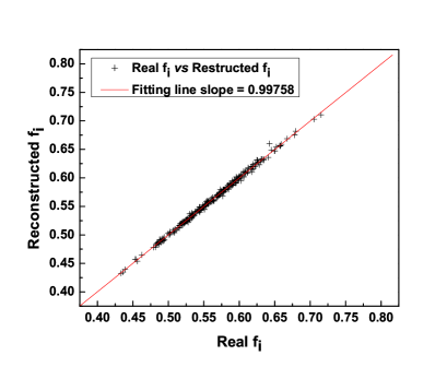
(a)Linear regression between $f_{i}({\rm x},t)$ and $\widehat{f}_{i}({\rm x},t)$ (b)Linear regression between $f_{i}^{(\rm neq)}({\rm x},t)$ and $\widehat{f}_{i}^{(\rm neq)}({\rm x},t)$

Figure 1: Linear regression (D2Q9, $u_{0}=0.1$, $t=1000\delta t$, $i=2$): (a)Fit the line $\widehat{f}_{i}({\rm x},t)=af_{i}({\rm x},t)+b$,where $a=0.99758$ and $b=0.00135$;(b)Fit the line $\widehat{f}_{i}^{(\rm neq)}({\rm x},t)=af_{i}^{(\rm neq)}({\rm x},t)+b$,where $a=0.83265$ and $b=-2.95012\times 10^{-6}$. Standard deviation:(a)$\sigma=0.00308$;(b)$\sigma=9.21597\times 10^{-4}$.

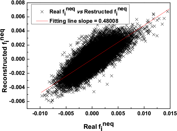
Figure 5: Linear regression (D2Q9, $u_{0}=0.1$, $t=1000\delta t$, $i=2$): Fit the line $\widehat{f}_{i}({\rm x},t)=af_{i}({\rm x},t)+b$,where $a=0.48088$ and $b=-0.248003\times 10^{-6}$.

In Figs (1)-(4), the reconstructed single-particle distribution functions and non-equilibrium distribution functions are compared with the real single-particle distribution functions and non-equilibrium distribution functions by linear regression analysis. When $u_{0}=0.1$ and $t=1000\delta t$, it is clear that the reconstructed single-particle distribution functions and the non-equilibrium distribution functions coincide with the real single-particle distribution functions and non-equilibrium distribution functions very well for D2Q9 and D2Q17 in Figs (1)-(2). The corresponding relative errors ${{\rm E}(f_{i},\widehat{f}_{i})}$ are about $0.242\%$ and $0.194\%$, respectively. The relative errors ${{\rm E}(f_{i}^{\rm(neq)},\widehat{f}_{i}^{\rm(neq)})}$ are about $16.735\%$ and $15.782\%$ for the single-particle non-equilibrium distribution functions of D2Q9 and D2Q17, respectively. If Eq.(60) by Imamura et al [31] is used to calculate the single-particle non-equilibrium distribution functions, the relative errors ${{\rm E}(f_{i}^{\rm(neq)},\widehat{f}_{i}^{\rm(neq)})}$ are up to about $21.65\%$ and $18.13\%$ for D2Q9 and D2Q17, respectively. We also adopted Eqs. (61) in [9] and (62)in [32] to do the same calculations. The relative errors ${{\rm E}(f_{i}^{\rm(neq)},\widehat{f}_{i}^{\rm(neq)})}$ of the single-particle non-equilibrium distribution functions can be up to about $80\%$ at many lattice nodes. In Fig. 5, the numerical relation between $f_{i}^{\rm(neq)}$ and $\widehat{f}_{i}^{\rm(neq)}$ for the method in [32]. The mean relative error ${\rm E}(f_{i}^{\rm(neq)},\widehat{f}_{i}^{\rm(neq)})$ is larger than $43.74\%$ for D2Q9. In the statistical procedure, we ignore the points with very small $f_{i}^{\rm(neq)}$ and $\widehat{f}_{i}^{\rm(neq)}$ ($f_{i}^{\rm(neq)},\widehat{f}_{i}^{\rm(neq)}<10^{-3}$) for the method in [32]. Here, we must point out that when $f_{i}^{\rm(neq)}$ and $\widehat{f}_{i}^{\rm(neq)}$ are very small, the relative errors ${\rm E}(f_{i}^{\rm(neq)},\widehat{f}_{i}^{\rm(neq)})$ of the methods in [9, 32] are very large. In such a circumstance, the relative error of the non-equilibrium distribution functions by Eq. (77) is also a bit larger, but it still less than that computed by Eq. (60) [31] and much less than that computed by Eqs. (61)$\sim$ (62) of [9] and [32], respectively. Similar results can be observed for the case of $u_{0}=0.01$ at $t=10000\delta t$ for D2Q9 and D2Q17. For the simplicity of presentation, they are not provided here.

In addition we also found that when the single-particle distribution functions and non-equilibrium distribution functions are reconstructed, the results from D2Q17 model show a better accuracy than that of D2Q9 model. Meanwhile, from the both models, more accurate results can be gained when the Mach number is reduced. Such results are very reasonable, and can be understood as follows. First, D2Q17 model is more accurate to approach Maxwell distribution function in discrete velocity spaces than D2Q9 model. Second, low Mach number will lead to a reduction of the truncated errors for approaching Maxwell distributions and a better recovering Navier-Stokes equation. It is proved [37] that D2Q17 model can eliminate the third-order term of statistical velocity in recovered Navier-Stokes equation.

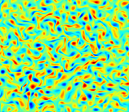
(a)Vorticity contour plot by the real $f_{i}({\rm x},t)$
(b)Vorticity contour plot by the reconstructed $\widehat{f}_{i}({\rm x},t)$

Figure 6: Vorticity contour plots (D2Q9, $u_{0}=0.1$, $t=1000\delta t$): (a)Vorticity contour plot by the real $f_{i}({\rm x},t)$ ; (b)Vorticity contour plot by the reconstructed $\widehat{f}_{i}({\rm x},t)$

Finally, attention is turned to the comparison of vorticity by the real ${f}_{i}({\rm x},t)$ and the reconstructed $\widehat{f}_{i}({\rm x},t)$ in Figs. 6$\sim$7, where the vorticity contour figures are given for $u_{0}=0.1$ and $u_{0}=0.01$, respectively.In order to show the quantitative sense of the vorticity reconstruction error, we choose 100 and 1000 time-series samples for $u_{0}=0.1$ and $u_{0}=0.001$, respectively. The $L^{2}$-relative departures of the reconstructed vorticity are $0.02\%\pm 0.0014\%$ (D2Q9, $u_{0}=0.1$), $0.005\%\pm 0.0003\%$ (D2Q17, $u_{0}=0.1$), $0.01\%\pm 0.0026\%$ (D2Q9, $u_{0}=0.01$) and $0.003\%\pm 0.0005\%$ (D2Q17, $u_{0}=0.01$). The agreement is very good.

In all, the proposed two operators can reconstruct the single-particle distribution functions and non-equilibrium distribution functions accurately and effectively. It can be shown that the two reconstruction operators are very flexible to apply to other discrete velocity models of lattice Boltzmann equation.

4.2 The rates of convergence

In order to validate the approach behaviors versus different grid sizes, we give the convergence properties of the D2Q9 and D2Q17 models by different mesh scales. The 2D Taylor-Green vortex problem is chosen as the intial fields

$$\left\{\begin{array}[]{ll}u=-&A{\rm cos}(k_{1}x){\rm sin}(k_{2}y)F(t)\\ v=&A\frac{k_{1}}{k_{2}}{\rm sin}(k_{1}x){\rm cos}(k_{2}y)F(t)\\ p=&p_{0}-\dfrac{A^{2}}{4}\left[{\rm cos}(2k_{1}x)+\dfrac{k_{1}^{2}}{k_{2}^{2}}{\rm cos}(2k_{2}y)\right]F^{2}(t)\end{array}\right.$$ (87)

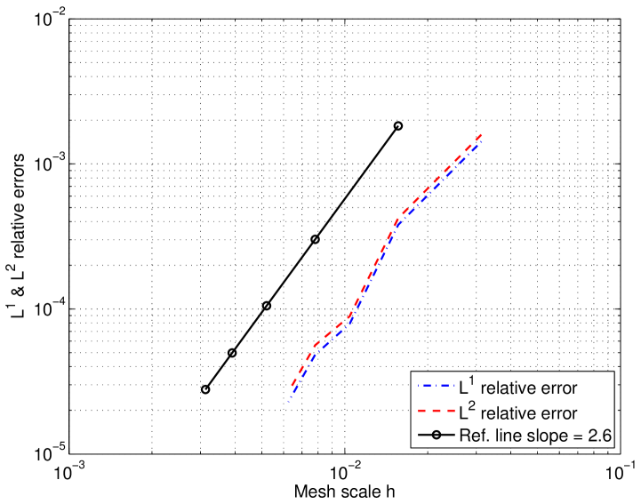
(a) the D2Q9 model
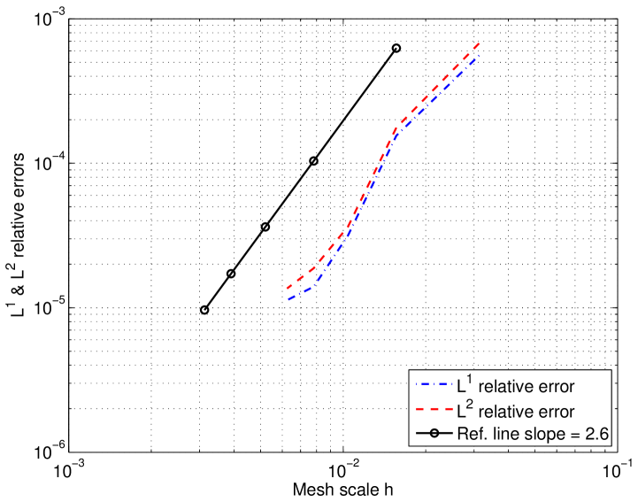
(b) the D2Q17 model

Figure 8: Convergence rates of the reconstruction operator for D2Q9 and D2Q17.

where $F(t)={\rm exp}\left[-\nu(k_{1}^{2}+k_{2}^{2})t\right]$, $A=0.1$, $k_{1}=k_{2}=4$ and $p_{0}=\rho_{0}c_{s}^{2}$. The computational domain $\Omega=[0,2\pi]^{2}$ and $Re=10000$. The periodic boundary conditions are applied in both directions. The initial distribution functions are initialized by the reconstruction operator. The reconstruction $L^{1}$ and $L^{2}$ relative errors of the distribution functions are calculated at the time steps $n=\{2000,4000,6000,8000,10000\}$ corresponding to the mesh resolutions $h=\{1/32,1/64,1/96,1/128,1/160\}$ respectively. In Fig. 8, the relative errors are given in the log-log coordinates. From the results, it is clear that for the D2Q9 model and the D2Q17 model, they nearly have the same convergence rates which are approximately equal to 2.6. However, the relative errors of the D2Q17 model are smaller than that of the D2Q9 model. That means the reconstruction precision can be improved when the number of the discrete velocity increases. This conclusion is consistent with the result in Sec. 4.1.

4.3 Coupling computations of FVM and LBM for lid-driven cavity flows

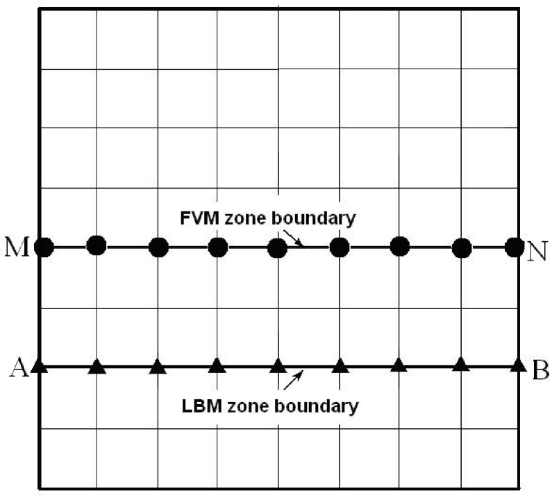
(a)Interface structure between two regions of FVM and LBM
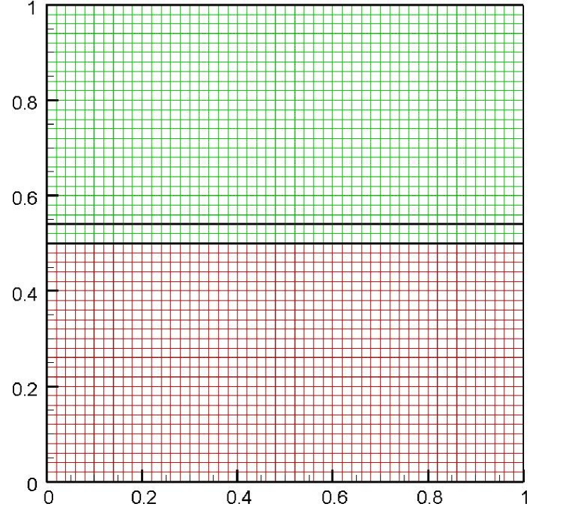
(b) Grid layout for a 2D lid-driven cavity ($200\times 200$)

Figure 9: Geometric structure and mesh partition: (a)Interface structure between two regions of FVM and LBM; (b)Grid layout for a 2D lid-driven cavity ($200\times 200$)

In order to illustrate the feasibility of the recommended reconstruction operator, the lid-driven cavity flow is simulated by the coupled LBM-FVM method. The computational domain is decomposed in two regions in which the LBM and FVM methods are used respectively (see Fig. 9-(a)). The coarseness and fineness of the grids can adjusted according to the zone spatial scale in each region. If the grid systems at the interface of overlap subregions are not identical, space interpolation at the interface is required when transferring the information at the interface. In this paper, the identical mesh structures are used for FVM and LBM for convenience to avoid the spatial interpolation (see Fig. 9-(b)). In order to implement the coupling computations, the overlap Schwartz alternative procedure is used to handle the computations.

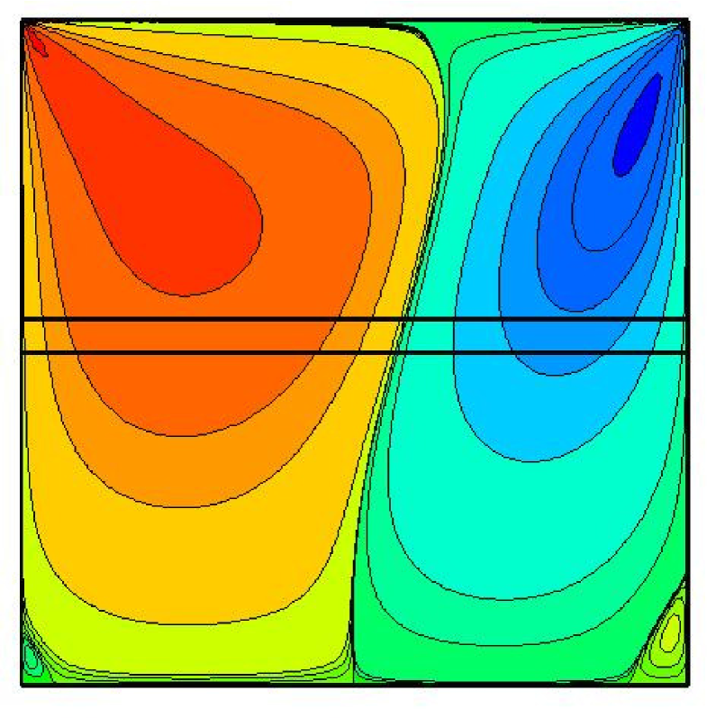
(a) $Re=100$     (b) $Re=400$     (c) $Re=1000$

Figure 14: Contour plots of vertical velocity for different Reynolds numbers

Numerical simulations were carried out for cavity flow of $Re=100,400$ and $1000$ on a grid $200\times 200$. The characteristic length of square cavity is $L=1$. The boundaries of the cavity are stationary walls, except the top-boundary with a uniform tangential velocity ($u_{t,Re=100}=3.33\times 10^{-3}$, $u_{t,Re=400}=1.33\times 10^{-3}$, $u_{t,Re=1000}=3.33\times 10^{-2}$). Fig. 10 shows plots of the stream function for the Reynolds number considered. These plots give a clear picture of the overall flow pattern and the effect of Reynolds number on the structure of the recirculating eddies in the cavity. The smoothness of the stream function distribution, especially around the overlap region confirms the correctness of the information transfer at the interface. To further quantify these results, the velocity profiles along the vertical and horizontal centerlines of the cavity are shown in Fig. 11. The results are in close agreement with the benchmark solution [39]. The smoothness and consistency of velocity distribution in the overlap region is presented in Fig. 12 where a local, enlarged view of the vector plot in the overlap region is shown. Clearly, the vectors in the overlap region are quiet consistent between the LBM results and the FVM results. Figs. 13 and 14 show the contours of horizontal and vertical velocity. It is seen that these physical quantities are all smooth across the interface. According to the authors’ numerical experience, the smoothness of vorticity contour is the most difficult to obtain for such coupled computation, because vorticity if the derivative of velocity. The contours of vorticity distribution are shown in Fig. 15. Over all, the smoothness on the overlap region are quite good, with a minor bumpiness of the left-hand vortex contours for the case of $Re=100$.

In all, by the proposed lifting relation, we can couple the mesoscopic LBM with FVM to implement the domain decomposition coupling-computations. This paves the way for implementing multiscale computations based on LBM and macro-numerical methods of finite-family.

It should be noted that we also tried the coupling computations based on the distribution function $f_{i}({\rm x},t)$ reconstructed by Eq. (61) of [9] and (62) of [32]. Unfortunately, all of our tries were unsuccessful and converged solutions could not be obtained.

Conclusion

In this paper, we derive the relation to lift the macroscopic variables to the microscopic variables for LBM. Two methods of derivation are conducted and they lead to the same result. Numerical tests demonstrate that the derived lifting relation possesses good precision. The proposed lifting relation offers a way to implement the multiscale-computations involving LBM more efficiently and robustly.

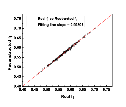
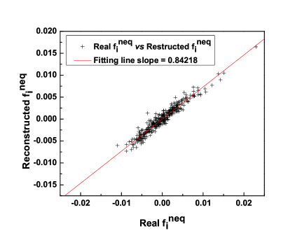
(a)Linear regression between $f_{i}({\rm x},t)$ and $\widehat{f}_{i}({\rm x},t)$ (b)Linear regression between $f_{i}^{(\rm neq)}({\rm x},t)$ and $\widehat{f}_{i}^{(\rm neq)}({\rm x},t)$

Figure 2: Linear regression (D2Q17, $u_{0}=0.1$ $t=1000\delta t$, $i=2$): (a)Fit the line $\widehat{f}_{i}({\rm x},t)=af_{i}({\rm x},t)+b$,where $a=0.99806$ and $b=0.00227$;(b)Fit the line $\widehat{f}_{i}^{(\rm neq)}({\rm x},t)=af_{i}^{(\rm neq)}({\rm x},t)+b$,where $a=0.84218$ and $b=-4.84408\times 10^{-6}$. Standard deviation:(a)$\sigma=0.00288$;(b)$\sigma=8.39673\times 10^{-4}$.

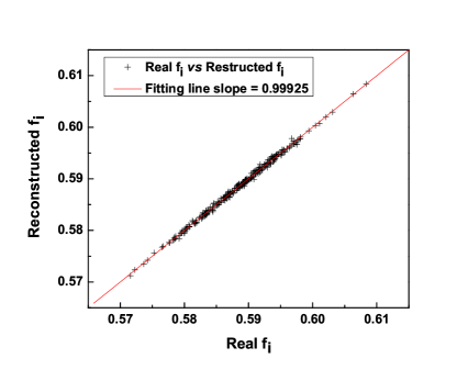
(a)(a)Linear regression between $f_{i}({\rm x},t)$ and $\widehat{f}_{i}({\rm x},t)$ (b)Linear regression between $f_{i}^{(\rm neq)}({\rm x},t)$

Figure 3: Linear regression (D2Q9, $u_{0}=0.01$, $t=10000\delta t$, $i=2$): (a)Fit the line $\widehat{f}_{i}({\rm x},t)=af_{i}({\rm x},t)+b$,where $a=0.99925$ and $b=4.41542\times 10^{-4}$;(b)Fit the line $\widehat{f}_{i}^{(\rm neq)}({\rm x},t)=af_{i}^{(\rm neq)}({\rm x},t)+b$,where $a=0.83655$ and $b=-1.51056\times 10^{-8}$. Standard deviation:(a)$\sigma=3.52548\times 10^{-4}$;(b)$\sigma=1.01264\times 10^{-4}$.

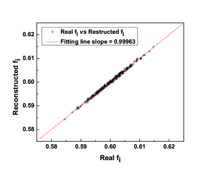
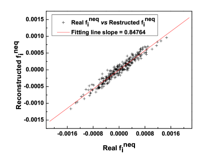
(a)Linear regression between $f_{i}({\rm x},t)$ and $\widehat{f}_{i}({\rm x},t)$ (b)Linear regression between $f_{i}^{(\rm neq)}({\rm x},t)$ and $\widehat{f}_{i}^{(\rm neq)}({\rm x},t)$

Figure 4: Linear regression (D2Q17, $u_{0}=0.01$, $t=10000\delta t$, $i=2$): (a)Fit the line $\widehat{f}_{i}({\rm x},t)=af_{i}({\rm x},t)+b$,where $a=0.99963$ and $b=2.17\times 10^{-4}$;(b)Fit the line $\widehat{f}_{i}^{(\rm neq)}({\rm x},t)=af_{i}^{(\rm neq)}({\rm x},t)+b$,where $a=0.84764$ and $b=-2.17758\times 10^{-8}$. Standard deviation:(a)$\sigma=3.37821\times 10^{-4}$;(b)$\sigma=9.47431\times 10^{-5}$.

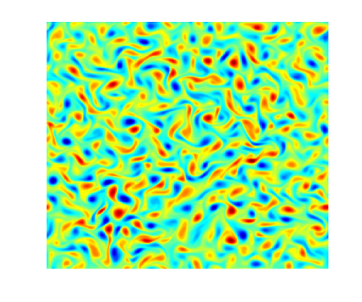
(a)Vorticity contour plot by the real $f_{i}({\rm x},t)$
(b)Vorticity contour plot by the reconstructed $\widehat{f}_{i}({\rm x},t)$

Figure 7: Vorticity contour plots (D2Q9, $u_{0}=0.01$, $t=10000\delta t$): (a)Vorticity contour plot by the real $f_{i}({\rm x},t)$ ; (b)Vorticity contour plot by the reconstructed $\widehat{f}_{i}({\rm x},t)$

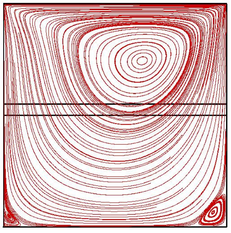
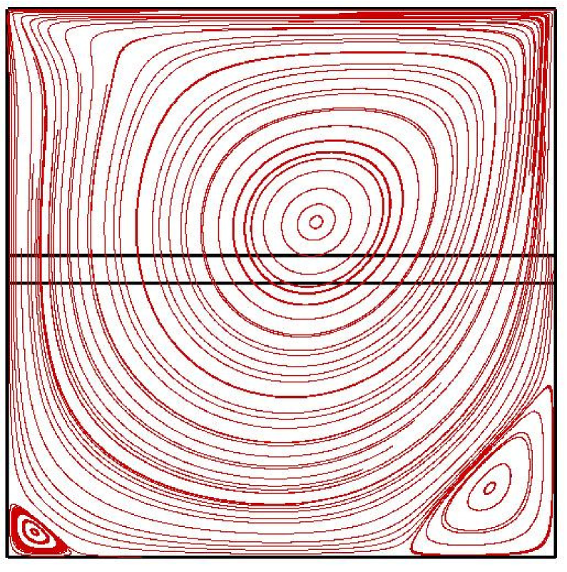
(a) $Re=100$     (b) $Re=400$     (c) $Re=1000$

Figure 10: Contour plots of streamline for different Reynolds numbers

(a) Horizontal velocity profiles

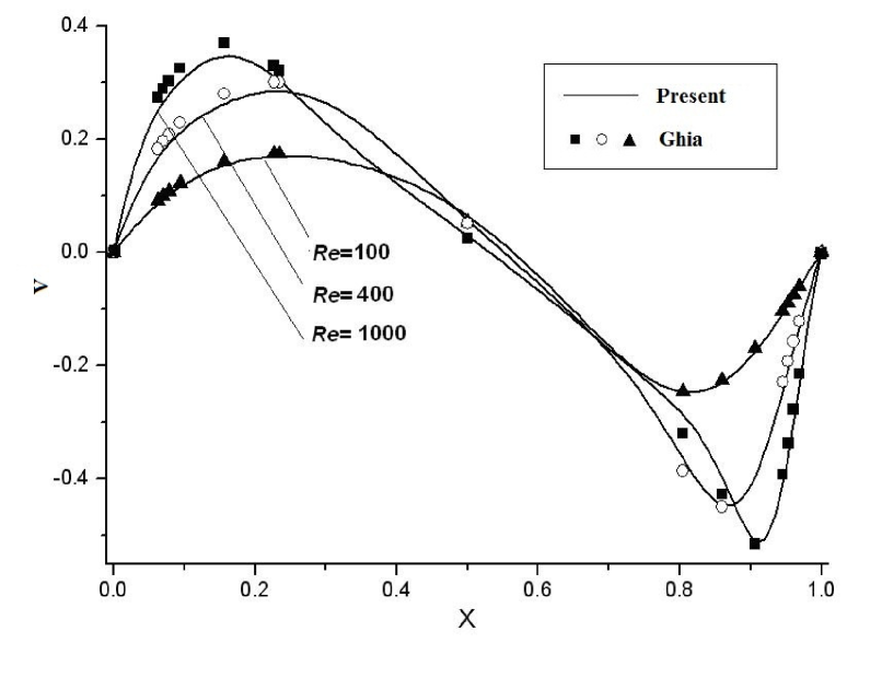
(b)Vertical velocity profiles

Figure 11: Comparisons between Ghia’s benchmark solutions and coupling solutions

(a) $Re=100$       (b) $Re=400$       (c) $Re=1000$

Figure 12: Enlarge vector plots in overlap regions

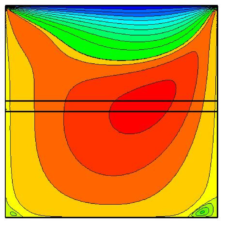
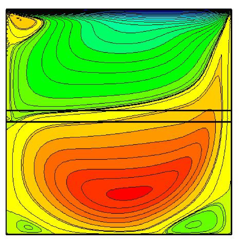
(a) $Re=100$     (b) $Re=400$     (c) $Re=1000$

Figure 13: Contour plots of horizontal velocity for different Reynolds numbers

(a) $Re=100$     (b) $Re=400$     (c) $Re=1000$

Figure 15: Contour plots of vorticity for different Reynolds numbers

References

- [1] R. Benzi, S. Succi and M. Vergassola, The lattice Boltzmann equation: theory and applications, Phys. Rep. 222 (1992) 145-197.
- [2] S. Succi, The Lattice Boltzmann Equation for Fluid Dynamics and Beyond. (Oxford Uniersity Press, Oxford, UK, 2001).
- [3] S. A. Orszag, H. Chen, S. Succi and J. Latt, Turbulence effects on kinetic equations J. Scie. Comput. 28(213) (2006) 459-466.
- [4] H. Chen, S. Kandasamy, S. A. Orszag, R. Shock, S. Succi and V.Yakhot, Extended Boltzmann kinetic equation for turbulent flows Science. 301 (2003) 633-636.
- [5] Q. J. Kang, D. X. Zhang and S. Y. Chen , Unified lattice boltzmann method for flow in multiscale porous media, Phys. Rev. E 66 (2002) 056307.
- [6] M. G. Fyta, S. Melchionna, E. Kaxiras and S. Succi, Multiscale coupling of molecular dynamics and hydrodynamics: application to DNA translocation through a nanopore, Multiscale Model. Sim. 5 (2006) 1156-1173.
- [7] S. Succi, O. Filippova, G. Smithand Kaxiras E., Applying the Lattice Boltzmann Equation to Multi-scale Fluid Problems, Computing in Science and Engineering, 3(6) (2001), 26-37.
- [8] A. Dupuis, E. M. Kotsalis and P. Koumoutsakos, Coupling Lattice Boltzmann and Molecular Dynamics Models for Dense Fluids, PHYSICAL REVIEW E, 75 (2007), 046704.
- [9] P. A. Skordos, Initial and boudary conditions for the lattice Boltzmann method, Phys. Rev. E 48(6) 1993, 4823-4841.
- [10] A. Caiazzo, Analysis of lattice Boltzmann initialization routines, J. Stat. Phys. 121 (2005), 37-48.
- [11] R. Mei, L.-S. Luo, P. Lallemand, and D. d’Humires, Consistent initial conditions for lattice Boltzmann simulations, Computers and Fluids 35 (8/9) (2006), 855-862.
- [12] A.A. Mohamad and S. Succi, A note on equilibrium boundary conditions in lattice Boltzmann fluid dynamic simulations, Eur. Phys. J. Special Topics 171 (2009) 213-221.
- [13] M. Junk and Z.X. Yang, Convergence of lattice Boltzmann methods for Navier-Stokes flows in periodic and bounded domains, Numerische Mathematik, 112(1) (2009) 65-87.
- [14] M. Junk and Z.X. Yang, Outflow boundary conditions for the lattice Boltzmann method, Progress in Computational Fluid Dynamics, 8(1/4) (2008) 38-48.
- [15] M. Junk and Z.X. Yang, Asymptotic analysis of lattice Boltzmann boundary conditions, J. Stat. Phys. 121 (2005) 3-35.
- [16] S. T. O’Connel, P. A. Thompson, Molecular dynamics-continuum hybrid computations: A tool for studying complex fluid flows, Physics Review E, 52 (6) (1995), R5792-R5795.
- [17] F F. Abraham Dynamically spanning the length scales from the quantum to the continuum, International Journal of Modern Physics C, 11 (6) (2000), 1135-1148.
- [18] J. Liu, S. Y. Chen, X. B. Nie and M. O. Robbins , A continuum atomistic simulation of heat transfer in micro- and nano-flow, J. computational Physics, 227 (2007), 279-291.
- [19] P. Albuquerque, D. Alemani, B. Chopard and P. Leone, Coupling a Lattice Boltzmann and a Finite Difference Scheme, Computational Science, ICCS- 04, Kracow, June 6-9, 2004. LCNS 3039, Bubak, M.; Albada, G.D.v.; Sloot, P.M.A.; Dongarra, J. (Eds.) Springer Verlag, Berlin.
- [20] P. Van Leemput, W. Vanroose and D. Roose, Numerical and analytical spatial coupling of a lattice Boltzmann model and a partial differential equation. In Model Reduction and Coarse-Graining Approaches for Multiscale Phenomena, (A.N. Gorban, N. Kazantzis, I.G. Kevrekidis, H.C. Ottinger, C. Theodoropoulos eds.), p. 423-441. Springer, 2006.
- [21] P. Van Leemput, W. Vanroose and D. Roose, Mesoscale analysis of the equation-free constrained runs initialization scheme, (SIAM) Multiscale Modeling and Simulation, 6 (4) (2007): 1234-1255.
- [22] I. G. Kevrekidis, C. W. Gear, J. M. Hyman, P. G. Kevrekidis, O. Runborg and C. Theodoropoulos, Equation-free, coase-grained multiscale computation: Enabling microscopic simulators to perform system-level analysis, Communications in Mathematical Science, 1(4) (2003) 715-762.
- [23] M. D. Mazzeo, P. V. Coveney, HemeLB: A high performance parallel lattice-Boltzmann code for large scale fluid flow in complex geometries, Computer Physics Communications, 178 (12) (2008): 894-914.
- [24] G. Amati, S. Succi, R. Piva, Massively Parallel Lattice-Boltzmann Simulation of Turbulent Channel Flow, International Journal of Modern Physics C, 8 (4) (1997): 869-877.
- [25] X. B. Nie, S. Y. Chen, W. N. E and M. O. Robbins, A continuum and molecular dynamics hybrid method for micro- and nano-fluid flow. J. Fluid Mech. 500 (2004), 55-64.
- [26] M. Junk, A. Klar, L. S. Luo Asymptotic analysis of the lattice Boltzmann equation, Journal of Computational Physics, 210 (2005) 676-704.
- [27] S. Chen, G. Doolen, Lattice Boltzmann method for fluid flows, Annu. Rev. Fluid Mech. 161 (1998) 329.
- [28] D. Ricot, V. Maillard, C. Bailly, Numerical simulation of unsteady cavity flow using Lattice Boltzmann Method, in: AIAA-Paper 2002-2532, 2002.
- [29] W. N. E and B. Engquist, The heterogeneous multiscale methods, Communications in Mathematical Science, 1(1) (2003) 87-133.
- [30] Z. L. Guo and C. G. Zheng, Theory and application of lattice Boltzmann Method. (Science Press, Beijing, 2008)
- [31] T. Imamura, K. Suzuki, T. Nakamura and M. Yoshida, Acceleration of steady-state lattice Boltzmann simulation on non-uniform mesh using local time step method, J. Comput. Phys. 202 (2005) 645-663.
- [32] Z. L. Guo and T. S. Zhao, Explicit finite-difference lattice Boltzmann method for curvilinear coordinates, Phys. Rev. E, 67 (2003) 066709.
- [33] S.Chapman and T. G. Cowling , The mathematical theory of nonuniform gases, 3rd. ed Cambridge University Press, Cambridge, 1970.
- [34] F. Schwabl, Statistical Mechanics, 2nd. ed, Springer-Verlag Berlin Heidelberg, (2006).
- [35] H.B. Luan, H. Xu, L. Chen, D. L. Sun, Y. L. He and W. Q. Tao, Evaluation of the coupling scheme of FVM and LBM for fluid flows around complex geometries, Int. J. Heat Mass Tran. 54 (2011), 1975-1985.
- [36] Y. H. Qian, D. d’Humieres, and P. Lallemand, Lattice BGK Models for Navier-Stokes Equation, Europhys. Lett., 17(6) (1992), 479-484.
- [37] Y.H. Qian and Y. Zhou, Complete Galilean-Invariant Lattice BGK Models for the Navier-Stokes Equation, Europhys. Lett., 42 (1998) 359-364.
- [38] J. R. Chasnov, On the decay of two-dimensional homogeneous turbulence, Phys. Fluids, 9(1) (1997) 171-180.
- [39] U. Ghia , K. N. Ghia, and C. T. Shin, High-Re Solutions for Incompressible Flow using the Navier-Stokes Equationuations and a Multigrid Method, J. Compt. Phys., 48 (1982) 387-411.