New Parameterized Algorithms for Edge Dominating Set

Abstract

An edge dominating set of a graph $G=(V,E)$ is a subset $M\subseteq E$ of edges in the graph such that each edge in $E-M$ is incident with at least one edge in $M$. In an instance of the parameterized edge dominating set problem we are given a graph $G=(V,E)$ and an integer $k$ and we are asked to decide whether $G$ has an edge dominating set of size at most $k$. In this paper we show that the parameterized edge dominating set problem can be solved in $O^{*}(2.3147^{k})$ time and polynomial space. We show that this problem can be reduced to a quadratic kernel with $O(k^{3})$ edges.

1 Introduction

The edge dominating set problem (EDS), to find an edge dominating set of minimum size in a graph, is one of the basic problems highlighted by Garey and Johnson in their work on NP-completeness [5]. It is known that the problem is NP-hard even when the graph is restricted to planar or bipartite graphs of maximal degree three [15]. The problem in general graphs and in sparse graphs has been extensively studied in approximation algorithms [15, 4, 1]. Note that a maximum matching is a 2-approximation for EDS. The 2-approximation algorithm for the weighted version of EDS is considerably more complicated [4].

Recently, EDS also draws much attention from the exact - and parameterized algorithms community. Randerath and Schiermeyer [9] designed an $O^{*}(1.4423^{m})$ algorithm for EDS which was improved to $O^{*}(1.4423^{n})$ by Raman et al. [10]. Here $n$ and $m$ are the number of vertices and edges in the graph. Fomin et al., [3] further improved this result to $O^{*}(1.4082^{n})$ by considering the treewidth of the graph. Rooij and Bodlaender [11] designed an $O^{*}(1.3226^{n})$ algorithm by using the ‘measure and conquer method.’

For parameterized edge dominating set (PEDS) with the parameter $k$ being the size of the edge dominating set, Fernau [2] gives an $O^{*}(2.6181^{k})$ algorithm. Fomin et al. [3] obtain an $O^{*}(2.4181^{k})$-time and exponential-space algorithm based on dynamic programming on bounded treewidth graphs. Unfortunately, their paper only briefly sketches the description and analysis of this algorithm.

Faster algorithms are known for graphs that have maximal degree three. The EDS and PEDS problems in degree-3 graphs can be solved in $O^{*}(1.2721^{n})$ [13] and $O^{*}(2.1479^{k})$ [14].

In this paper, we present two new algorithms for PEDS. The first one is a simple and elegant algorithm that runs in $O^{*}(2.3715^{k})$ time and polynomial space. We improve the running-time bound to $O^{*}(2.3147^{k})$ by using a technique that deals with remaining graphs of maximal degree three. We also design a linear-time algorithm that obtains a quadratic kernel which is smaller than previously-known kernels.

Our algorithms for PEDS are based on the technique of enumerating minimal vertex covers. We introduce the idea of the algorithms in Section 2 and introduce some basic techniques in Section 3. We present a simple algorithm for PEDS in Section 4 and an improved algorithm in Section 5. We moved the proof of a technical lemma to Appendix 0.A. In Section 6 we discuss the problem kernel.

2 Enumeration-based algorithms

As in many previous algorithms for the edge dominating set problem [2, 3, 11, 13] our algorithms are based on the enumeration of minimal vertex covers. Note that the vertex set of an edge dominating set is a vertex cover. Conversely, let $C$ be a minimal vertex cover and $M$ be a minimum edge dominating set containing $C$ in the set of its endpoints. Given $C$, $M$ can be computed in polynomial time by computing a maximum matching in induced graph $G[C]$ and adding an edge for each unmatched vertex in $C$. This observation reduces the problem to that of finding the right minimal vertex cover $C$. Now, the idea is to enumerate all minimal vertex covers. Moon and Moser showed that the number of minimal vertex covers is bounded by $3^{n/3}$ and this shows that one can solve EDS in $O(1.4423^{n})$ time [6, 7].

For PEDS, we want to find an edge dominating set of size bounded by $k$. It follows that we need to enumerate minimal vertex covers of size only up to $2k$. We use a branch-and-reduce method to find vertex covers. We fix some part of a minimal vertex cover and then we try to extend it with at most $p$ vertices. Initially $p=2k$. In fact, in our algorithms, we may not really enumerate all minimal vertex covers of size up to $p$. But we will guarantee that at least one of the right vertex covers will be considered if a solution exists.

For a subset $C\subseteq V$ and an independent set $I\subseteq V-C$ in $G$, an edge dominating set $M$ is called a $(C,I)$-eds if

$$C\subseteq V(M)\quad\text{and}\quad I\cap V(M)=\varnothing.$$

In the search for the vertex cover $V(M)$ of a minimum $(C,I)$-eds $M$, we keep track of a partition of the vertices of $G$ in four sets: $C$, $I$, $U_{1}$ and $U_{2}$. Initially $C=I=U_{1}=\varnothing$ and $U_{2}=V$. The following conditions are kept invariant.

1. $I$ is an independent set in $G$, and

2. each component of $G[U_{1}]$ is a clique component of $G[V\setminus(C\cup I)]$.

The vertices in $U_{1}\cup U_{2}$ are called undecided vertices. We use a five-tuple

$$(G,C,I,U_{1},U_{2})$$

to denote the state described above. We let $q_{i}=|Q_{i}|$ denote the number of vertices of a clique component $Q_{i}$ of $G[U_{1}]$. Rooij and Bodlaender proved the following lemma in [11].

Lemma 1

If $U_{2}=\varnothing$ then a minimum $(C,I)$-eds $M$ of $G$ can be found in polynomial time.

When there are no undecided vertices in the graph we can easily find a minimum $(C,I)$-eds. Lemma 1 tells us that clique components in the undecided graph $G[V\setminus(C\cup I)]$ do not cause trouble. We use some branching rules to deal with vertices in $U_{2}$.

Consider the following simple branching rule. For any vertex $v\in U_{2}$ consider two branches that either include $v$ into the vertex cover or exclude $v$ from the vertex cover. In the first branch we move $v$ into $C$. In the second branch we move $v$ into $I$ and move the set $N(v)$ of neighbors of $v$ into $C$.

When we include a number of vertices into the vertex cover, we reduce the parameter $p$ by the same value. Furthermore, in each branch we move any newly-found clique component $Q$ in $G[U_{2}]$ into $U_{1}$ and reduce $p$ by $|V(Q)|-1$. The reason is that each clique has at most one vertex that is not in the vertex cover.

Let $C(p)$ denote the worst-case running time to enumerate vertex covers up to size $p$. Then we have the following inequality:

$$C(p)\leq C(p-1-q_{v})+C(p-|N(v)|-q_{N(v)}),$$ (1)

where $q_{v}$ (resp., $q_{N(v)}$) denotes the sum of $|V(Q)|-1$ over all cliques $Q$ in $G[U_{2}]$ that appear after removing $v$ (resp., $N(v)$) from $U_{2}$.

At worst, both $q_{v}$ and $q_{N(v)}$ are 0. Then we end up with the recurrence

$$C(p)\leq C(p-1)+C(p-|N(v)|).$$

Note that one can always branch on vertices of degree at least $2$ in $G[U_{2}]$. In this manner Fernau [2] solves the edge dominating set problem in $O^{*}(1.6181^{p})=O^{*}(2.6181^{k})$ time which stems from the solution of the Fibonacci recurrence

$$C(p)\leq C(p-1)+C(p-2).$$

Fomin et.al., [3] refine this as follows. Their algorithm first branches on vertices in $G[U_{2}]$ of degree at least $3$ and then it considers the treewidth of the graph when all the vertices in $G[U_{2}]$ have degree one or two. If the treewidth is small the algorithm solves the problem by dynamic programming and if the treewidth is large the algorithm branches further on vertices of degree two in $G[U_{2}]$. This algorithm uses exponential space and its running time depends on the running time of the dynamic programming algorithms.

The method of iteratively branching on vertices of maximum degree is powerful when this is more than two. Unfortunately, it seems that we can not avoid some branchings on vertices of degree $2$, especially when each component of $G[U_{2}]$ is a $2$-path, i.e., a path that consists of two edges. We say that we are in the worst case when every component of $G[U_{2}]$ is a $2$-path.

Our algorithms branch on vertices of maximum degree and on some other local structures in $G[U_{2}]$ until $G[U_{2}]$ has only $2$-path components. When we are in the worst case our algorithms deal with the graph in the following way. Let $P=v_{0}v_{1}v_{2}$ be a $2$-path in $G[U_{2}]$. We say $P$ is signed if $v_{1}\in V(M)$, and unsigned if $v_{1}\not\in V(M)$. We use an efficient way to enumerate all signed $2$-paths in $G[U_{2}]$.

In the next section we introduce our branching rules.

3 Branching rules

Besides the simple technique of branching on a vertex, we also use the following branching rules. Recall that in our algorithm, once a clique component $Q$ appears in $G[U_{2}]$, we move $V(Q)$ into $U_{1}$ and reduce $p$ by $|V(Q)|-1$.

3.0.1 Tails

Let the vertex $v_{1}$ have degree two. Assume that $v_{1}$ has one neighbor $v_{0}$ of degree one and that the other neighbor $v_{2}$ has degree $>1$. Then we call the path $v_{0}v_{1}v_{2}$ a tail.

In this paper, when we use the notation $v_{0}v_{1}v_{2}$ for a tail, we implicitly mean that the first vertex $v_{0}$ is the degree-$1$ vertex of the tail. Branching on a tail $v_{0}v_{1}v_{2}$ means that we branch by including $v_{2}$ into the vertex cover or excluding $v_{2}$ from the vertex cover.

Lemma 2

If $G[U_{2}]$ has a tail then we can branch with the recurrence

$$C(p)\leq 2C(p-2)\quad\Rightarrow\quad C(p)=O(1.4143^{p}).$$ (2)

Proof

Let the tail be $v_{0}v_{1}v_{2}$. In the branch where $v_{2}$ is included into $C$, $\{v_{0},v_{1}\}$ becomes a clique component and this is moved into $U_{1}$. Then $p$ reduces by $1$ from $v_{2}$ and by $1$ from $\{v_{0},v_{1}\}$. In the branch where $v_{2}$ is included into $I$, $N(v_{2})$ is included into $C$. Since $|N(v_{2})|\geq 2$, $p$ also reduces by $2$ in this branch. ∎

3.0.2 $4$-Cycles

We say that $abcd$ is a $4$-cycle if there exist the four edges $ab$, $bc$, $cd$ and $da$ in the graph. Xiao [12] used the following lemma to obtain a branching rule for the maximum independent set problem. In this paper we use it for the edge dominating set problem.

Lemma 3

Let $abcd$ be a $4$-cycle in graph $G$, then any vertex cover in $G$ contains either $a$ and $c$ or $b$ and $d$.

As our algorithm aims at finding a vertex cover, it branches on a $4$-cycle $abcd$ in $G[U_{2}]$ by including $a$ and $c$ into $C$ or including $b$ and $d$ into $C$. Notice that we obtain the same recurrence as in Lemma 2.

4 A simple algorithm

Our first algorithm is described in Fig. 1. The search tree consists of two parts. First, we branch on vertices of maximum degree, tails and $4$-cycles in Lines 3-4 until every component in $G[U_{2}]$ is a $2$-path. Second, we enumerate the unsigned $2$-paths in $G[U_{2}]$. In each leaf of the search tree we find an edge dominating set in polynomial time by Lemma 1. We return a smallest one.

   Algorithm $$EDS(G,C,I,U_{1},U_{2},p) G=(V,E) V C I U_{1} U_{2} C=I=U_{1}=\varnothing U_{2}=V p p=2k \leq k G Q G[U_{2}] U_{1} p |Q|-1 p<0 4 G[U_{2}] Q G[U_{2}] 2 v Q P 2 G[U_{2}] y=|P| y>\min(p,k) z=\min(p-y,k-y) P^{\prime}\subseteq P 0\leq|P^{\prime}|\leq z v_{0}v_{1}v_{2}\in P^{\prime} \{v_{0},v_{2}\} C v_{1} U_{1} v_{0}v_{1}v_{2}\in P-P^{\prime} v_{1} C \{v_{0},v_{2}\} U_{1} M U_{2}=\varnothing C\cup I\cup U_{1}=V$$
Input: A graph , and a partition of into sets , , and . Initially , . Integer ; initially .
Output: An edge dominating set of size in if it exists.
1. While there is a clique component in do move it into and reduce by . 2. If then halt. 3. While there is a tail or -cycle in do branch on it. 4. If there is component of that is not a -path then pick a vertex of maximum degree in and branch on it. 5. Else let be the set of -paths in and . 6. If then halt. 7. Let . 8. For each subset of size do For each do move into and move into ;
For each do move into and move into . 9. Compute the candidate edge dominating set and return the smallest one.     (Here , )   

Figure 1: Algorithm $EDS(G,C,I,U_{1},U_{2},p)$

4.1 Analysis

To show the correctness of the algorithm we explain Line 6 and Line 8.

For each $2$-path in $G[U_{2}]$ we need at least one edge to dominate it. So, we must have that $y\leq p$ and $y\leq k$. This explains the condition in Line 6.

It is also easy to see that for each unsigned $2$-path we need at least two different edges to dominate it. Let $p^{\prime}$ be the number of unsigned $2$-paths. In Line 8, we enumerate the possible sets $P^{\prime}\subseteq P$ of unsigned $2$-paths. Notice that

$$(y+p^{\prime}\leq k\;\;\text{and}\;\;y+p^{\prime}\leq p)\quad\Leftrightarrow\quad p^{\prime}\leq z.$$

We analyze the running time of this algorithm. Lemma 1 guarantees that the subroutine in Line $9$ runs in polynomial time. We focus on the exponential part of the running time. We prove a bound of the size of the search tree in our algorithm with respect to measure $p$.

First, we consider the running time of Lines 3-4.

Lemma 4

If the graph has a vertex of degree $\geq 3$ then Algorithm $EDS$ branches with

$$C(p)\leq C(p-1)+C(p-3)\quad\Rightarrow\quad C(p)=O(1.4656^{p}).$$ (3)

Proof

If the algorithm branches on a tail or a $4$-cycle we have the upperbound given by (2). Else the algorithm branches on a vertex of maximum degree and generates a recurrence covered by (3). Notice that (3) covers (2). This proves the lemma. ∎

Lemma 5

If all components of the graph are paths and cycles then the branchings of Algorithm $EDS$ before Line 5 satisfy (3).

Proof

If there is a path component of length $>2$, then there is a tail and the algorithm branches on it with (2).

If there is a component $C_{l}$ which is an $l$-cycle in $G[U_{2}]$, the algorithm deals with it in this way: If the cycle is a $3$-cycle, the algorithm moves it into $U_{1}$ without branching since it is a clique.

If the cycle is a $4$-cycle then, according to Lemma 3, our algorithm branches on it with (2).

If the cycle has length at least $5$, our algorithm selects an arbitrary vertex $v_{0}$ and branches on it. Subsequently it branches on the path that is created as long as the length of the path is greater than $2$. When the cycle is a $5$-cycle we obtain the recurrence

$$C(p)\leq 3C(p-3)\quad\Rightarrow\quad C(p)=O(1.4423^{p}).$$

When the cycle is a $6$-cycle we obtain the recurrence

$$C(p)\leq C(p-2)+C(p-3)+C(p-4)\quad\Rightarrow\quad C(p)=O(1.4656^{p}).$$

The two recurrences above are covered by (3). Straightforward calculations show that when the cycle has length $\geq 7$, we also get a recurrence covered by (3). For brevity we omit the details of this analysis. ∎

By Lemma 4 and Lemma 5 we know that the running time of the algorithm, before it enters Line 5 is $O^{*}(1.4656^{x})$, where $x$ is the size of $C$ upon entering the loop in Line 8. We now consider the time that is taken by the loop in Line 8 and then analyze the overall running time.

First we derive a useful inequality.

Lemma 6

Let $r$ be a positive integer. Then for any integer $0\leq i\leq\lfloor\frac{r}{2}\rfloor$

$${r-i\choose i}=O(1.6181^{r}).$$ (4)

Proof

Notice that

$$\binom{r-i}{i}\leq\sum_{i=0}^{\lfloor\frac{r}{2}\rfloor}\binom{r-i}{i}=F(r+1),$$

where $F(r)$ is the $r^{\mathrm{th}}$ Fibonacci number. We have $F(r)=O(1.6181^{r})$. ∎

Now we are ready to analyze the running time of the algorithm. It is clear that the loop in Line 8 takes less than $y{y\choose z}$ basic computations. First assume that $x\leq k$. We have that $z\leq k-y$ thus $y+z\leq k$. If we apply Lemma 6 with $r=y+z$ we find that the running time of the loop in Line 8 is $O^{*}(1.6181^{k})$. By Lemmas 4 and 5 the running time of the algorithm is therefore bounded by $O^{*}(1.4656^{x}\cdot 1.6181^{k})=O^{*}(2.3715^{k})$.

Assume that $x>k$. We now use that $z\leq p-y$ thus $y+z\leq p$. By Lemma 6 the running time of Step 8 is $O^{*}(1.6181^{p})$. Now $p\leq 2k-x$ and $x>k$. The running time of the algorithm is therefore bounded by

$$O^{*}(1.4656^{x}\cdot 1.6181^{p})=O^{*}(2.3715^{k}).$$

We summarize the result in the following theorem.

Theorem 4.1

Algorithm $EDS$ solves the parameterized edge dominating set problem in $O^{*}(2.3715^{k})$ time and polynomial space.

5 An improvement

In this section we present an improvement on Algorithm $EDS$. The improved algorithm is described in Fig. 2.

The search tree of this algorithm consists of three parts. First, we iteratively branch on vertices of degree $\geq 4$ until $G[U_{2}]$ has no such vertices anymore (Line $3$). Then we partition the vertices in $U_{2}$ into two parts: $V(P)$ and $U_{2}^{\prime}$, where $P$ is the set of $2$-path components in $G[U_{2}]$ and $U_{2}^{\prime}=U_{2}\setminus V(P)$. Then the algorithm branches on vertices in $U_{2}^{\prime}$ until $U_{2}^{\prime}$ becomes empty (Line $4$-$5$). Finally, we enumerate the number of unsigned $2$-paths in $P$ (Line $9$) and continues as in Algorithm $EDS$.

In Algorithm $EDS1$ a subroutine $Branch3$ deals with some components of maximum degree $3$. It is called in Line 5. This is the major difference with Algorithm $EDS$. Algorithm $Branch3$ is described in Fig. 3. The algorithm contains several simple branching cases. They could be described in a shorter way but we avoided doing that for analytic purposes.

We show the correctness of the condition in Line 7 of Algorithm $EDS1$. The variable $p_{0}$ in Algorithm $PEDS1$ marks the decrease of p by subroutine $Branch3$. Note that no vertices in $V(P)$ are adjacent to vertices in $U^{\prime}_{2}$. Let $M_{1}$ be the set of edges in the solution with at least one endpoint in $U_{2}^{\prime}$ and let $M_{2}$ be the set of edges in the solution with at least one endpoint in $V(P)$. Then

$$M_{1}\cap M_{2}=\emptyset\quad\text{and}\quad|M_{1}|+|M_{2}|\leq k\quad\text{and}\quad|M_{1}|\geq\frac{p_{0}}{2}.$$

Thus $|M_{2}|\leq k-\frac{p_{0}}{2}$. The correctness of Algorithm $EDS1$ now follows since the only difference is the subroutine $Branch3$.

   Algorithm $$EDS1(G,C,I,U_{1},U_{2},p) G=(V,E) V C I U_{1} U_{2} C=I=U_{1}=\varnothing U_{2}=V p p=2k \leq k G Q G[U_{2}] U_{1} p |Q|-1 p<0 v \geq 4 G[U_{2}] P 2 G[U_{2}] U_{2}^{\prime}=U_{2}\setminus V(P) y=|P| p^{\prime}=p U_{2}^{\prime}\neq\varnothing p\geq 0 (G,C,I,U_{1},U_{2},p)=Branch3(G,C,I,U_{1},U_{2}=U^{\prime}_{2}\cup V(P),p) p_{0}=p^{\prime}-p y>\min(p,k-p_{0}/2) z=\min(p-y,k-p_{0}/2-y) P^{\prime}\subseteq P 0\leq|P^{\prime}|\leq z v_{0}v_{1}v_{2}\in P^{\prime} \{v_{0},v_{2}\} C v_{1} U_{1} v_{0}v_{1}v_{2}\in P-P^{\prime} v_{1} C \{v_{0},v_{2}\} U_{1} M U_{2}=\varnothing C\cup I\cup U_{1}=V$$
Input: A graph and a partition of into sets , , and . Initially , . Integer ; initially .
Output: An edge dominating set of size in if it exists.
1. While there is a clique component in do move it into and decrease by . 2. If halt. 3. While there is a vertex of degree in do branch on it. 4. Let denote the set of -path components in and . Let and . 5. While and do . 6. Let . 7. If halt. 8. Let . 9. For each subset of size do for each do move into and move into ;
for each do move into and move into . 10. Compute the candidate edge dominating set and return the smallest one.     (Here , .)   

Figure 2: Algorithm $EDS1(G,C,I,U_{1},U_{2},p)$

   Algorithm $$Branch3(G,C,I,U_{1},U_{2}=U^{\prime}_{2}\cup V(P),p) G[U^{\prime}_{2}] U_{1} 2 v_{0}v_{1}v_{2} G[U^{\prime}_{2}] v_{1} U^{\prime}_{2}\neq\varnothing 3 v 1 G[U^{\prime}_{2}] v v_{0}v_{1}v_{2} v_{2} 2 G[U^{\prime}_{2}] v_{0}v_{1}v_{2} v_{2} 3 G[U^{\prime}_{2}] 3 v 1 G[U^{\prime}_{2}] v 4 G[U^{\prime}_{2}] 3 v 2 G[U^{\prime}_{2}] v v G[U^{\prime}_{2}] 2 v_{0}v_{1}v_{2} v_{1}$$
1. If there is a clique component in then move it to . 2. If there is a -path component in then branch on . 3. If then 3.1 If there is a degree- vertex adjacent to two degree- vertices in then branch on . 3.2 If there is a tail such that is a degree- vertex in then branch on the tail. 3.3 If there is a tail such that is a degree- vertex in then branch on the tail. 3.4 If there is a degree- vertex adjacent to one degree- vertex in then branch on . 3.5 If there is a -cycle in then branch on it. 3.6 If there is a degree- vertex adjacent to any degree- vertex in then branch on . 3.7 Pick a maximum vertex in and branch on it. In addition to 3.1–3.7: * If some -path component is created in 3.1 – 3.7 then branch on .   

Figure 3: Algorithm $Branch3(G,C,I,U_{1},U_{2},p)$

5.1 Analysis of Algorithm $EDS1$

We put the proof of the following lemma in Appendix 0.A.

Lemma 7

The branchings of Algorithm $Branch3$ satisfy the recurrence

$$C(p)\leq C(p-2)+2C(p-3)\quad\Rightarrow\quad C(p)=O(1.5214^{p}).$$ (5)

Algorithm $EDS1$ first branches on vertices of degree at least $4$. These branchings of the algorithm satisfy

$$C(p)\leq C(p-1)+C(p-4)\quad\Rightarrow\quad C(p)=O(1.3803^{p}).$$ (6)

Recall that the subroutine $Branch3$ reduces $p$ by $p_{0}$. The analysis without the subroutine is similar to the analysis of Algorithm $EDS$ in Section 4.1 except that $k$ is replaced by $k-\frac{p_{0}}{2}$ and that Formula (3) is replaced by Formula (6). Thus without the subroutine $Branch3$ the algorithm has a run-time proportional to

$$(1.3803\cdot 1.6181)^{k-\frac{p_{0}}{2}}=2.2335^{k-\frac{p_{0}}{2}}.$$

By Lemma 7 the running time of the algorithm is therefore bounded by

$$O^{*}(2.2335^{k-p_{0}/2}\cdot 1.5214^{p_{0}})=O^{*}(2.2335^{k-p_{0}/2}\cdot 2.3147^{p_{0}/2})=O^{*}(2.3147^{k}).$$

This proves the following theorem.

Theorem 5.1

Algorithm $EDS1$ solves the parameterized edge dominating set problem in $O^{*}(2.3147^{k})$ time and polynomial space.

6 Kernelization

A kernelization algorithm takes an instance of a parameterized problem and transforms it into an equivalent parameterized instance (called the kernel), such that the new parameter is at most the old parameter and the size of the new instance is a function of the new parameter.

For the parameterized edge dominating set problem Prieto [8] presented a quadratic-time algorithm that finds a kernel with at most $4k^{2}+8k$ vertices by adapting ‘crown reduction techniques.’ Fernau [2] obtained a kernel with at most $8k^{2}$ vertices.

We present a new linear-time kernelization that reduces a parameterized edge dominating set instance $(G,k)$ to another instance $(G^{\prime},k^{\prime})$ such that

$$|V(G^{\prime})|\leq 2k^{\prime 2}+2k^{\prime}\quad\text{and}\quad|E(G^{\prime})|=O(k^{\prime 3})\quad\text{and}\quad k^{\prime}\leq k.$$

In our kernelization algorithm we first find an arbitrary maximal matching $M_{0}$ in the graph in linear time. Let $m=|M_{0}|$, then we may assume that $m\geq k+1$ otherwise $M_{0}$ solves the problem directly. Let

$$V_{m}=V(M_{0})\quad\text{and}\quad V^{*}=V-V_{m}.$$

Since $M_{0}$ is a maximal matching, we know that $V^{*}$ is an independent set. For a vertex $v_{i}\in V_{m}$, let $x_{i}=|V^{*}\cap N(v_{i})|$. We call vertex $v_{i}\in V_{m}$ overloaded, if $m+x_{i}>2k$. Let $A\subseteq V_{m}$ be the set of overloaded vertices.

Lemma 8

Let $M$ be an edge dominating set $M$ of size at most $k$. Then

$$A\subseteq V(M).$$

Proof

If an overloaded vertex $v_{i}\not\in V(M)$ then all neighbors of $v_{i}$ are in $V(M)$. Note that at least one endpoint of each edge in $M_{0}$ must be in $V(M)$ and that $V^{*}\cap N(v_{i})$ and $V(M_{0})$ are disjoint. Therefore, $|V(M)|\geq x_{i}+m$. Since $v_{i}$ is an overloaded vertex we have that $|V(M)|>2k$. This implies that $|M|>k$ which is a contradiction. ∎

Lemma 8 implies that all overloaded vertices must be in the vertex set of the edge dominating set. We label these vertices to indicate that these vertices are in the vertex set of the edge dominating set.

We also label a vertex $v$ which is adjacent to a vertex of degree one.

Our kernelization algorithm is presented in Fig. 4. In the algorithm the set $A^{\prime}$ denotes the set of labeled vertices. The correctness of the algorithm follows from the following observations. Assume that there is a vertex $u$ only adjacent to labeled vertices. Then we can delete it from the graph without increasing the size of the solution. The reason is this. Let $ua$ be an edge that is in the edge dominating set of the original graph where $a$ is a labeled vertex. Then we can replace $ua$ with another edge that is incident with $a$ to get an edge dominating set of the new graph. This is formulated in the reduction rule in Line 4 of the algorithm. We add a new edge for each labeled vertex in Line 5 to enforce that the labeled vertices are selected in the vertex set of the edge dominating set.

   Algorithm $$Kernel(G,k) M_{0} G A A^{\prime}=A v\in V_{m} 1 v 1 A^{\prime}\leftarrow A^{\prime}\cup\{v\} u\in V^{*} N(u)\subseteq A^{\prime} u G w\in A^{\prime} w_{i}^{\prime} w_{i}^{\prime}w_{i} w_{i}^{\prime} V^{*} (G^{\prime},k^{\prime}=k) G^{\prime}$$
1. Find a maximal matching in . 2. Find the set of overloaded vertices and let . 3. If there is a vertex that has a degree- neighbor then delete ’s degree- neighbors from the graph and let . 4. If there is a vertex such that then delete from . 5. For each vertex add a new vertex and a new edge
(In the analysis we assume that the new vertex is in ). 6. Return , where is the new graph.   

Figure 4: Algorithm $Kernel(G,k)$

It is easy to see that each step of the algorithm can be implemented in linear time. Therefore, the algorithm takes linear time.

We analyze the number of vertices in the new graph $G^{\prime}$ returned by Algorithm $Kernel(G,k)$. Note that $A^{\prime}$ is a subset of $V_{m}$. Let $B=V_{m}-A^{\prime}$. Let $q$ be the number of edges between $V^{*}$ and $B$. Then

$$q=\sum_{v_{i}\in B}x_{i}\leq\sum_{v_{i}\in B}(2k-m)=|B|(2k-m).$$

Let

$$V^{*}_{1}=\bigcup_{v\in B}N(v)\cap V^{*}\quad\text{and}\quad V^{*}_{2}=V^{*}-V^{*}_{1}.$$

Each vertex in $V^{*}_{1}$ is adjacent to a vertex in $B$. Since there are at most $q$ edges between $V^{*}_{1}$ and $B$ we have

$$|V^{*}_{1}|\leq q.$$

Notice that all vertices of $V^{*}_{2}$ have only neighbors in $A^{\prime}$. In Line 4 the algorithm deletes all vertices that have only neighbors in $A^{\prime}$. In Line 5 the algorithm adds a new vertex $v^{\prime}$ and a new edge $v^{\prime}v$ for each vertex $v$ in $A^{\prime}$. Thus $V^{*}_{2}$ is the set of new vertices that are added in Line 5. This proves

$$|V^{*}_{2}|=|A^{\prime}|=2m-|B|.$$

The total number of vertices in the graph is

$$\begin{array}[]{*{20}lll}|V_{m}|+|V^{*}_{1}|+|V^{*}_{2}|&\leq&2m+|B|(2k-m)+(2m-|B|)&\\ {}&=&4m+|B|(2k-m-1)&\\ {}&\leq&4m+2m(2k-m-1)&\quad\text{since $|B|\leq 2m$}\\ {}&=&2m(2k-m+1)&\\ {}&\leq&2k(k+1)&\quad\text{since $m\geq k+1$.}\\ \end{array}$$

Note that the maximal value of $2m(2k-m+1)$ as a function of $m$ is attained for $m=k+\frac{1}{2}$. So the function $2m(2k-m+1)$ is decreasing for $m\geq k+1$.

To obtain a bound for the number of edges we partition the edge set into three disjoint sets.

1. Let $E_{1}$ be the set of edges with two endpoints in $V_{m}$;

2. let $E_{2}$ be the set of edges between $A^{\prime}$ and $V^{*}$, and

3. let $E_{3}$ be the set of edges between $B$ and $V^{*}$.

It is easy to see that

$$|E_{1}|=O(m^{2})=O(k^{2})\quad\text{and}\quad|E_{3}|=q=|B|(2k-m)=O(k^{2}).$$

By the analysis above

$$|E_{2}|\leq|A^{\prime}|\times|V^{*}_{1}|+|V^{*}_{2}|\leq|A^{\prime}|q+|V^{*}_{2}|\quad\Rightarrow\quad|E_{2}|=O(k^{3}).$$

Lemma 9

Algorithm $Kernel$ runs in linear time and linear space and it returns a kernel with at most $2k^{2}+2k$ vertices and $O(k^{3})$ edges.

7 Related problems

There are standard techniques to reduce the parameterized maximal matching problem that finds a maximal matching of size $k$ in a graph to the parameterized edge dominating set problem without increasing the input size and the parameter [15]. By Theorem 5.1 we have

Corollary 1

The parameterized maximal matching problem can be solved in $O^{*}(2.3147^{k})$ time and polynomial space.

Another related problem is the parameterized matrix domination problem. Let $M$ be an $m\times n$ matrix with entries being $0$ or $1$ and let $k$ be an integer $k$. The problem is to find a subset $S$ of the $1$-entries in $M$ such that $|S|\leq k$ and every row and column of $M$ contains at least one $1$-entry in $S$. A parameterized matrix domination instance reduces directly to a parameterized edge dominating set problem in a bipartite graph [15, 2].

Corollary 2

The parameterized matrix domination problem can be solved in $O^{*}(2.3147^{k})$ time and polynomial space.

Appendix 0.A Analysis of Algorithm $Branch3$

In this section, we analyze Algorithm $Branch3$ presented in Fig. 3 and we prove Lemma 7. Initially $G[U_{2}^{\prime}]$ contains no component that is a 2-path. We prove that in each line of Step 3, Algorithm $Branch3$ branches with (5), or with a better recurrence, without leaving any newly-created 2-path components. To be exact, some 2-path components may be created but they are removed immediately by an application of Line 2 in the following step. In the analysis we merge these operations into one recurrence. We limit the number of $2$-paths that are created in each step to prove the upperbound on the run-time.

Lemma 10

If there is a path component $P$ of length $l$ in $G[U^{\prime}_{2}]$ then Algorithm $Branch3$ branches with the following recurrences until $U_{2}^{\prime}$ contains no more vertices of $P$.

$$C(p) \leq C(p-1)+C(p-2)\quad\Rightarrow\quad C(p)=O(1.6181^{p}) l=2$$ for (7)

$$C(p) \leq C(p-2)+C(p-2)\quad\Rightarrow\quad C(p)=O(1.4143^{p}) l=3$$ for (8)

$$C(p) \leq C(p-2)+C(p-3)\quad\Rightarrow\quad C(p)=O(1.3248^{p}) l=4$$ for (9)

$$C(p) \leq 2C(p-3)+C(p-4)\quad\Rightarrow\quad C(p)=O(1.3954^{p}) l=5$$ for (10)

$$C(p) \leq C(p-3)+3C(p-4)\quad\Rightarrow\quad C(p)=O(1.4527^{p}) l=6$$ for (11)

$$C(p) \leq 3C(p-4)+C(p-5)\quad\Rightarrow\quad C(p)=O(1.3888^{p}) l=7$$ for (12)

$$C(p) \leq 3C(p-5)+4C(p-6)\quad\Rightarrow\quad C(p)=O(1.4220^{p}) l\geq 8$$ for . (13)

Proof

Let $P$ be the path $p_{0}p_{1}\cdots p_{l}$. The algorithm branches on tails of paths. It is easy to see that Formulas (7), (8) and (9) hold. When $l=5$, we first branch on $p_{2}$. In the branch where $p_{2}$ is included into the vertex cover $C$, we get a clique component $p_{0}p_{1}$ and a $2$-path $p_{3}p_{4}p_{5}$. Then we can further reduce $p$ by at least one from $p_{0}p_{1}$ and branch with (7) on $p_{3}p_{4}p_{5}$. In the branch where $p_{2}$ is included into the independent set $I$, $p_{1}$ and $p_{3}$ are included into $C$ and we end up with two clique component $p_{0}$ and $p_{4}p_{5}$. Then $p$ reduces further by at least one from $p_{4}p_{5}$. Summarizing the above leads to Formula (10).

When $l\geq 6$ then, no matter whether $p_{2}$ is included into the vertex cover $C$ or not, $p$ reduces by at least two. Then, in the first branch the algorithm branches further on an $(l-3)$-path and in the second branch it branches further on an $(l-4)$-path. This leads to Formulas (11) and (12).

To prove Formula (13) we use induction on $l$. Assume that for all $l<l_{0}$ the inequality holds true. we prove that (13) also holds true for $l=l_{0}$, where $l_{0}>7$. In the branch where $p_{2}$ is included into the vertex cover $C$, the algorithm branches further on an $(l_{0}-3)$-path. In the branch where $v_{2}$ is not included into the vertex cover, the algorithm continues branching on an $(l_{0}-4)$-path. We have that $l_{0}-4\geq 4$. The worst recurrence among (9), (10), (11), (12) and (13) is Formula (11) and the second worst recurrence is Formula (13). Furthermore, (10) is worse than (12). Thus the two branches that occur after branching on $v_{2}$ are bounded as follows.

1. In the two subbranches we further branch with (10) and (11)

2. in both of the two subbranches we further branch with (13).

The final recurrences created by the above two worst cases are covered by (13). This proves the claim. ∎

Assume that $G[U_{2}^{\prime}]$ contains a component which is a cycle $C=v_{0}\ldots v_{l-1}$ of length $l$. If the cycle is a $3$-cycle, the algorithm moves it to $U_{1}$ without branching since it is a clique. If the cycle is a $4$-cycle then according to Lemma 3 the algorithm branches with Formula (2). If the cycle is a cycle of length at least five, the algorithm selects a vertex and branches on it. Subsequently, it branches on the paths created in each subbranch. By Lemma 10 we obtain the following recurrences for $C_{l}$.

Lemma 11

If there is a cycle-component $C$ of length $l$ in $G[U^{\prime}_{2}]$ the algorithm branches with the following recurrences.

$$\text{$l=4$:}\;\;C(p) \leq C(p-2)+C(p-2)\;\Rightarrow\;\;C(p)=O(1.4143^{p})$$ (14)

$$\text{$l=5$:}\;\;C(p) \leq 3C(p-3)\;\Rightarrow\;\;C(p)=O(1.4423^{p})$$ (15)

$$\text{$l=6$:}\;\;C(p) \leq 2C(p-3)+2C(p-4)\;\Rightarrow\;\;C(p)=O(1.4946^{p})$$ (16)

$$\text{$l\geq 7$:}\;\;C(p) \leq C(p-5)+6C(p-6)+4C(p-7)\;\Rightarrow\;\;C(p)=O(1.4724^{p}).$$ (17)

Proof

Straightforward computations yield Formulas (14), (15) and (16). We prove (17). In the two branches we get two paths of length $l-2$ and $l-4$. Formulas (11) and (13) are the two worst recurrences among (8), (9), (10), (11), (12) and (13). This gives Formula (17). ∎

Lemma 12

The branching in Line 3.1 of Algorithm $Branch3$ (together with the branching on all $2$-paths that are created) generate

$$C(p)\leq C(p-2)+2C(p-3)\quad\Rightarrow\quad C(p)=O(1.5214^{p}).$$ (18)

Proof

Assume $v$ is a degree-$3$ vertex with two degree-$1$ neighbors in $G[U_{2}^{\prime}]$. The algorithm selects $v$ and branches; either it includes $v$ into $C$ or it includes $v$ into $I$ (and adds $\{u_{1},u_{2},u_{3}\}$ to $C$). We are interested in the number of $2$-paths that are created in each branch. In the first branch at most one $2$-path component is created. If this occurs then the second branch creates no $2$-path.

Let the pair $(a,b)$ denote that there are $a$ $2$-paths created in the first branch and $b$ $2$-paths created in the second branch. Then the possible values for $(a,b)$ are $(0,0)$, $(1,0)$, $(0,1)$ and $(0,2)$.

Once a $2$-path component is created the algorithm branches on it. In the first case this gives a recurrence $C(p)\leq C(p-1)+C(p-3)$ and it leaves no $2$-path component. In the second case the algorithm branches with

$$C(p)\leq C(p-1-1)+C(p-1-2)+C(p-3)=C(p-2)+2C(p-3),$$

and it leaves no $2$-paths. In the third case the algorithm branches with

$$C(p) \leq C(p-1)+C(p-3-1)+C(p-3-2)=$$

$$= C(p-1)+C(p-4)+C(p-5)$$

$$\Rightarrow C(p)=O(1.4971^{p}).$$

This case leaves no $2$-paths. It is easy to see the above three recurrences are covered by (18).

When the fourth case occurs there are only three possible cases for the component that contains $v$. We illustrate the three cases $a$, $b$ and $c$ in Fig. 5.

In Case $a$ the first branch after deleting $v$ has a path of length $6$ and then the algorithm branches further according to recurrence (11). In the second branch the algorithm branches further on two $2$-paths with the recurrence

$$C(p) \leq C(p-1-1)+C(p-1-2)+C(p-2-1)+C(p-2-2)=$$

$$= C(p-2)+2C(p-3)+C(p-4).$$

Summarizing, we get

$$C(p)\leq C(p-4)+4C(p-5)+2C(p-6)+C(p-7)\;\;\Rightarrow\;\;C(p)=O(1.4876^{p}).$$

In Case $b$ the first branch after deleting $v$ causes the algorithm to branch further on a degree-$3$ vertex and so on. We obtain the recurrence

$$C(p) \leq C(p-1-1)+C(p-1-3)+C(p-3-1)+C(p-3-2)=$$

$$= C(p-2)+2C(p-4)+C(p-5).$$

In the second branch of Case $b$ the algorithm branches further on two $2$-paths. Putting these together we obtain

$$C(p)\leq C(p-3)+3C(p-5)+3C(p-6)+C(p-7)\;\;\Rightarrow\;\;C(p)=O(1.5042^{p}).$$

In Case $c$, in the first branch after deleting $v$ the algorithm branches on a degree-$3$ vertex and so on. This yields

$$C(p) \leq C(p-1-2)+C(p-1-2)+C(p-3-1)+C(p-3-2)=$$

$$= 2C(p-3)+C(p-4)+C(p-5).$$

In the second branch of Case $c$ the algorithm branches on two $2$-paths. If we take them together we get

$$C(p) \leq 2C(p-4)+2C(p-5)+3C(p-6)+C(p-7)$$

$$\Rightarrow C(p)=O(1.4941^{p}).$$

Since the solution of (18) satisfies $C(p)=O(1.5214^{p})$, it follows that (18) covers all the cases.

This proves the lemma. ∎

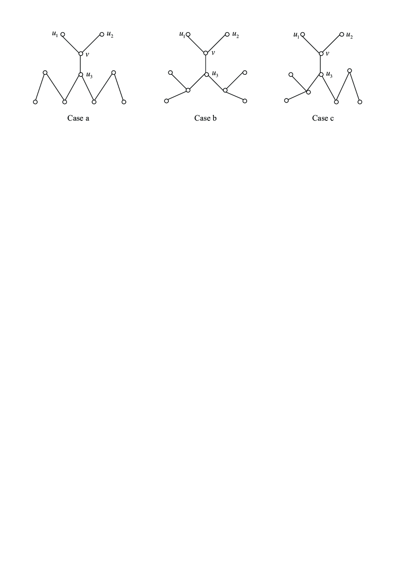
Figure 5: The three possible graphs for Case $(0,2)$

Lemma 13

In Line 3.2 of Algorithm $Branch3$ the algorithm branches with

$$C(p)\leq C(p-2)+2C(p-3).$$

Proof

Assume that $v_{0}v_{1}v_{2}$ is the tail and $v_{2}$ is a degree-$2$ vertex in $G[U^{\prime}_{2}]$. The algorithm branches on $v_{2}$ by including it into $C$ or including it into $I$ (and including its neighbors into $C$).

We consider the number of $2$-paths that are created in each branch. If the component that contains the tail is a $5$-path, then the algorithm branches on it according to Recurrence (10). Otherwise, it is impossible to create a $2$-path component after removing $v_{2}$.

There are at most two $2$-path components created in the second branch since there is no degree-$3$ vertex adjacent to two degree-$1$ vertices. If only one $2$-path component is created, the algorithm branches according to

$$C(p) \leq C(p-2)+C(p-2-1)+C(p-2-2)=$$

$$= C(p-2)+C(p-3)+C(p-4).$$

If two $2$-path components are created the algorithm branches with

$$C(p) \leq C(p-2)+C(p-2-2)+2C(p-2-3)+C(p-2-4)=$$

$$= C(p-2)+C(p-4)+2C(p-5)+C(p-6).$$

All the recurrences above are weaker than $C(p)\leq C(p-2)+2C(p-3)$. This proves the lemma. ∎

Lemma 14

In Line 3.3 of Algorithm $Branch3$ the algorithm branches with

$$C(p)\leq C(p-2)+2C(p-3).$$

Proof

The proof of Lemma 14 is similar to the proof of Lemma 15. ∎

Lemma 15

In Line 3.4 of Algorithm $Branch3$ the algorithm branches with

$$C(p)\leq C(p-2)+2C(p-3).$$

Proof

Assume that $v$ is a degree-$3$ vertex having one degree-$1$ neighbor in $G[U^{\prime}_{2}]$. The algorithm branches on $v$ by including it into $C$ or including it into $I$. Since Line 3.1 and Line 3.2 do no longer apply we can simply assume that in $G[U^{\prime}_{2}]$ there is no more degree-$3$ vertex adjacent to two degree-$1$ vertices nor any tail $v_{0}v_{1}v_{2}$ with $v_{2}$ being a degree-$2$ vertex.

Under this assumption we analyze the number of $2$-path components created in each branch.

Let $u_{0}u_{1}u_{2}$ be a $2$-path created after removing $v$ (or $N(v)$). Then there are at least two edges between $\{u_{0},u_{1},u_{2}\}$ and $v$ (or $N(v)$) otherwise, before branching on $v$ the condition of Line 3.1 or Line 3.2 holds. This implies that, after removing $v$, at most one $2$-path component is created.

If a $2$-path component is created in the first branch then no $2$-path component is created in the other branch. Therefore the branching of the algorithm satisfies

$$C(p) \leq C(p-1-1)+C(p-1-2)+C(p-3)=$$

$$= C(p-2)+2C(p-3).$$

If no $2$-path component is created in the first branch then at most two $2$-path components are created in the second branch. In the worst case we first branch on the degree-$3$ vertex $v$ and then branch on two $2$-path components in the second branch with

$$C(p)\leq C(p-2)+2C(p-3)+C(p-4).$$

Therefore, we get

$$C(p)\leq C(p-1)+C(p-5)+2C(p-6)+C(p-7)\;\;\Rightarrow\;\;C(p)=O(1.5181^{p}).$$ (19)

It follows that the worst recurrence is $C(p)\leq C(p-2)+2C(p-3)$. ∎

Lemma 16

In Line 3.5 of Algorithm $Branch3$ the algorithm branches with

$$C(p)\leq C(p-2)+2C(p-3).$$

Proof

Let $v_{1}v_{2}v_{3}v_{4}$ be a $4$-cycle in $G[U^{\prime}_{2}]$, the algorithm branches by including $v_{1}$ and $v_{3}$ or by including $v_{2}$ and $v_{4}$ into the vertex cover. Note that after Line 3.5 there are no more degree-$1$ vertices in $G[U^{\prime}_{2}]$. Thus in each branch at most one $2$-path component is created. Therefore, the algorithm branches first with $C(p)\leq 2C(p-2)$ for the $4$-cycle and then it possibly branches further on a $2$-path in each branch. This leads to the recurrence

$$C(p) \leq C(p-2-1)+C(p-2-2)+C(p-2-1)+C(p-2-2)=$$

$$= 2C(p-3)+2C(p-4)$$

$$\Rightarrow C(p)=O(1.4946^{p}).$$

This is covered by $C(p)\leq C(p-2)+2C(p-3)$. ∎

Lemma 17

In Line 3.6 of Algorithm $Branch3$ the algorithm branches with

$$C(p)\leq C(p-2)+2C(p-3).$$

Proof

Assume that $v$ is a degree-$3$ vertex adjacent to at least one degree-$2$ neighbor in $G[U^{\prime}_{2}]$. The algorithm branches on $v$ by including it into $G$ or $I$.

In the first branch no $2$-path is created otherwise there is a $4$-cycle in $G[U^{\prime}_{2}]$ before the branching on $v$.

In the second branch, where $N(v)$ is moved into $C$, there are at most two $2$-path components created. Note that for any $2$-path component $u_{0}u_{1}u_{2}$ that is created after removing $N(v)$ there are at least two edges between $\{u_{0},u_{1},u_{2}\}$ and $N(v)$, and at least one vertex in $N(v)$ is a degree-$2$ vertex. Therefore, we have (19) as an upperbound. ∎

Now we are ready to complete the proof of Lemma 7.

Proof

Notice that Lemmas 12, 13, 14, 15, 16 and 17 guarantee that, if any of the Lines 3.1 - 3.6 are called, the algorithm branches according to Formula (5).

In Line 3.7 the induced subgraph $G[U^{\prime}_{2}]$ has only two kinds of components: each component is either a cycle or a $3$-regular graph without any $4$-cycle. Lemma 11 proves that the branching on a cycle gives a recurrence which is no worse than (5).

Now we may assume that there are only $3$-regular components. In this case the algorithm selects an arbitrary vertex $v$ and branches on it. According to the analysis in the proof of Lemma 17 no $2$-path components are created after removing $v$. In the branch where $N(v)$ is removed at most one $2$-path is created. Note that for any $2$-path component $u_{0}u_{1}u_{2}$, created after removing $N(v)$, there are five edges between $\{u_{0},u_{1},u_{2}\}$ and $N(v)$, because each vertex is a degree-$3$ vertex before the branching. In the worst case the algorithm still branches with

$$C(p) \leq C(p-1)+C(p-3-1)+C(p-3-2)=$$

$$= C(p-1)+C(p-4)+C(p-5).$$

This is weaker than Formula (5).

Therefore, the branching of Algorithm $Branch3$ satisfies (5). ∎

References

- [1] Cardinal, J., S. Langerman, E. Levy, Improved approximation bounds for edge dominating set in dense graphs, Theor. Comput. Sci. 410 (2009), pp. 949–957.
- [2] Fernau, H., Edge dominating set: Efficient enumeration-based exact algorithms, In (H. Bodlaender, M. Langston eds.), Proceedings IWPEC, Springer-Verlag LNCS 4169 (2006), pp. 142–153.
- [3] Fomin, F., S. Gaspers, S. Saurabh, A. Stepanov, On two techniques of combining branching and treewidth, Algorithmica 54(2) (2009), pp. 181–207.
- [4] Fujito, T., H. Nagamochi, A 2-approximation algorithm for the minimum weight edge dominating set problem, Discrete Applied Mathematics 118(3) (2002), pp. 19–207.
- [5] Garey, M.R., D. S. Johnson, Computers and intractability: A guide to the theory of NP-completeness, Freeman, San Francisco, 1979.
- [6] Johnson, D., M. Yannakakis, C. Papadimitriou, On generating all maximal independent sets, Information Processing Letters 27(3) (1988), pp. 119–123.
- [7] Moon, J. W. and L. Moser, On cliques in graphs, Israel J. Math. 3 (1965), pp. 23–28.
- [8] Prieto, E., Systematic kernelization in FPT algorithm design, PhD-thesis, The University of Newcastle, Australia, 2005.
- [9] Randerath, B., I. Schiermeyer, Exact algorithms for minimum dominating set. Technical Report zaik 2005-501, Universität zu Köln, Germany, 2005.
- [10] Raman, V., S. Saurabh, S. Sikdar, Efficient exact algorithms through enumerating maximal independent sets and other techniques, Theory of Computing Systems 42(3) (2007), pp. 563–587.
- [11] Rooij, J. M., H. L. Bodlaender, Exact algorithms for edge domination, In (M. Grohe, R. Niedermeier, eds.), Proceedings IWPEC, Springer-Verlag LNCS 5018 (2008), pp. 214–225.
- [12] Xiao, M., A simple and fast algorithm for maximum independent set in 3-degree graphs, In (Md. S. Rahman and S. Fujita, eds.), Proceedings WALCOM, Springer-Verlag LNCS 5942 (2010), pp. 281–292.
- [13] Xiao, M., H. Nagamochi, Exact algorithms for annotated edge dominating set in cubic graphs. TR 2011-009. Kyoto University. 2011. A preliminary version appeared as: M. Xiao, Exact and parameterized algorithms for edge dominating set in 3-degree graphs, In (W. Wu, O. Daescu, eds.), Proceedings COCOA, Springer-Verlag LNCS 6509 (2010), pp. 387–400.
- [14] Xiao, M., H. Nagamochi, Parameterized edge dominating set in cubic graphs, Proceedings FAW-AAIM, Springer-Verlag LNCS 6681 (2011).
- [15] Yannakakis, M., F. Gavril, Edge dominating sets in graphs, SIAM J. Appl. Math. 38(3) (1980), pp. 364–372.