A Bayesian analysis of the nucleon QCD sum rules

Abstract

QCD sum rules of the nucleon channel are reanalyzed, using the maximum entropy method (MEM). This new approach, based on the Bayesian probability theory, does not restrict the spectral function to the usual “pole + continuum”-form, allowing a more flexible investigation of the nucleon spectral function. Making use of this flexibility, we are able to investigate the spectral functions of various interpolating fields, finding that the nucleon ground state mainly couples to an operator containing a scalar diquark. Moreover, we formulate the Gaussian sum rule for the nucleon channel and find that it is more suitable for the MEM analysis to extract the nucleon pole in the region of its experimental value, while the Borel sum rule does not contain enough information to clearly separate the nucleon pole from the continuum.

1 Introduction

The use of QCD sum rules in studies investigating the properties of baryons has already a long history. Since the seminal papers of Shifman et al. Shifman , in which the QCD sum rule method was developed and the subsequent first application to baryonic channels by Ioffe Ioffe , the sum rules of the nucleon have been continuously improved by including higher orders in the perturbative Wilson coefficients Krasnikov ; Chung2 ; Jamin ; Ovchinnikov ; Shiomi ; Sadovnikova or non-perturbative power corrections Belyaev ; Chung2 ; Leinweber1 . This even lead to attempts to determine the mass difference between the neutron and the proton Yang , which certainly is a very difficult task because of the smallness of this difference compared to hadronic scales. Another important development was initiated in a paper by Leinweber Leinweber2 , in which, among other technical points, the choice of the interpolating field made by Ioffe was criticized and a new statistical method for the analysis of QCD sum rules was introduced. Furthermore, QCD sum rules also have been used to investigate the nucleon properties in nuclear matter Hatsuda ; Cohen ; Drukarev or at finite temperature Adami .

However, in all these studies it was necessary to model the spectral function according to some specific functional form, the “pole + continuum”-ansatz being the most popular one. Such a procedure inevitably incorporates strong assumptions on the spectral function into the analysis. This strategy works well when the actual spectral function has some resemblance with the chosen model, but will of course fail if this is not the case. For instance, as is known from studies using both QCD sum rules and lattice QCD, certain linear combinations of interpolating fields, which in principle carry the quantum numbers of the nucleon, couple to the nucleon ground state only very weakly. A QCD sum rule analysis of such interpolating fields, which uses the “pole + continuum” ansatz, can only lead to ambiguous results. The problems become even more severe in studies of the spectral function at finite temperature or density, as the validity of the phenomenological ”pole + continuum” ansatz for the spectral function in such an environment becomes less certain, rendering it more difficult to make educated guesses about its actual form.

To avoid the above mentioned problems, and to reduce the assumptions that have to be made on the functional form of the spectral function, we have developed a novel method of analyzing QCD sum rules, which employs the maximum entropy method (MEM) Gubler1 . The method, which is based on Bayesian probability theory, was shown to give reasonable results in the analysis of the sum rule of the $\rho$-meson channel. Moreover, recently this approach was successfully applied to the charmonium sum rules at both zero and finite temperatures Gubler2 .

In this paper, it is our main purpose to examine if and to what extent the MEM analysis can be applied to the sum rule of the nucleon. Throughout our investigations, we found that the MEM analysis of the Borel sum rule

$$G_{\mathrm{OPE}}(M)=\frac{1}{M^{2}}\int^{\infty}_{0}dte^{-\frac{t}{M^{2}}}\rho(t),$$ (1)

in fact fails to satisfactorily extract the nucleon spectral function in the ground state region. As we will discuss later in detail, this failure is mainly caused by the large contribution of the continuum to the OPE side of Eq.(1), which strongly deteriorates the contribution of the nucleon pole.

On the other hand, the Gaussian sum rule Bertlmann ; Orlandini

$$G_{\mathrm{OPE}}(s,\tau)=\frac{1}{\sqrt{4\pi\tau}}\int^{\infty}_{0}dte^{-\frac{(t-s)^{2}}{4\tau}}\rho(t),$$ (2)

which, for the nucleon, is formulated for the first time in this paper, turns out to give better results and allows us to resolve the nucleon pole from the continuum. There are essentially two reasons for the superiority of the sum rule of Eq.(2). First of all, the kernel of Eq.(2), a Gaussian centered at $s$ with a width of $\sqrt{2\tau}$, collects more information on the spectral function $\rho(t)$ than the one in Eq.(1) when the integration over $t$ is carried out. This is especially true for small values of the width $\tau$, which we, however, cannot take arbitrarily small because below a certain threshold, the convergence of the operator product expansion (OPE) becomes poor. A similar situation occurs in the Borel sum rules, where the Borel mass is restricted from below due to the OPE convergence. The second reason also can be related to the kernel of Eq.(2), containing two parameters $s$ and $\tau$, which can be freely chosen as long as the OPE converges. This freedom allows us to vary two parameters at the same time in the MEM analysis of Gubler1 , leading to reasonable results for the extracted spectral function. Similar experiences also have been made in nuclear structure studies, where the Lorentz kernel has proven to be useful Efros ; Efros2 .

Furthermore, using the MEM analysis of the Gaussian sum rules, we are able to extract the spectral function not only in cases where the interpolating field strongly couples to the nucleon ground state and thus the “pole + continuum” ansatz should be valid, but also in cases where only higher energy states contribute to the sum rules and hence the conventional analysis most likely fails to give meaningful results. This advantage is especially useful for examining which kind of interpolating field couples strongly to the nucleon ground state and is thus a suitable interpolating field for the analysis, a question with a long and controversial history in QCD sum rules studies Ioffe ; Chung1 ; Chung3 ; Ioffe2 ; Dosch ; Leinweber2 . Our MEM analysis of the general operator given in Eq.(5) strongly suggests that the nucleon ground state only couples to $\eta_{1}(x)$ ($\beta=0$) and not to $\eta_{2}(x)$ ($\beta=\infty$)(see Eqs.(3) and (4) in Sec. 2). In addition, we have obtained some hints of excited states coupling to $\eta_{2}(x)$. These issues will be discussed in detail in Section 5.3.

The paper is organized as follows. In Sec. 2, the details of the Borel and Gaussian sum rule for the nucleon are explained. Next, the maximum entropy method (MEM) is elucidated in Sec. 3, after which in Sec. 4, the results of the analysis using the Borel sum rule in combination with MEM are presented. In Sec. 5, the results of the analysis for the Gaussian sum rule are outlined, and in Sec. 5.3, the differences of the obtained spectral functions depending on the choice of the interpolating fields are discussed. Finally, the summary and conclusions are given in Sec. 6.

2 QCD sum rules for the nucleon

The method of QCD sum rules is used to carry out the analysis of the spectral function as follows. First, we choose an interpolating field which has the quantum numbers of the nucleon, then its correlation function is calculated in the deep Euclidean 4-momentum region. Alternatively, the same correlation function at the physical 4-momentum region is expressed by the spectral function of the nucleon channel. The sum rules can then be constructed by equating the two expressions using a dispersion relation.

For the nucleon, there are two independent local interpolating operators,

$$\eta_{1}(x)=\epsilon^{abc}(u^{Ta}(x)C\gamma_{5}d^{b}(x))u^{c}(x),$$ (3)

$$\eta_{2}(x)=\epsilon^{abc}(u^{Ta}(x)Cd^{b}(x))\gamma_{5}u^{c}(x).$$ (4)

Here, $abc$ are color indices, $C$ is the charge conjugation matrix and $T$ stands for the transposition operation. The spinor indices are omitted for simplicity. A general interpolating operator can thus be expressed as

$$\eta(x)=\eta_{1}(x)+\beta\eta_{2}(x),$$ (5)

where $\beta$ is a real parameter. Here, the case of $\beta=-1$ is identified as the so-called “Ioffe current” Ioffe , which is often used in QCD sum rule studies of the nucleon.

Using this interpolating operator, we define the correlation function as

$$\begin{split}\Pi(q)&=i\int e^{iqx}\langle 0|T[\eta(x)\overline{\eta}(0)]|0\rangle d^{4}x\\ &=q/\Pi_{1}(q^{2})+\Pi_{2}(q^{2}).\end{split}$$ (6)

The imaginary part of $\Pi_{1}(q^{2})$ satisfies the positivity condition, $\mathrm{Im}\Pi_{1}(q^{2})\geq 0$, while $\mathrm{Im}\Pi_{2}(q^{2})$ is not necessarily positive due to contributions of negative parity states. The positivity condition is, however, essential for the application of the MEM method and we thus consider only $\Pi_{1}(q^{2})$ in the following. To make use of the information contained in $\mathrm{Im}\Pi_{2}(q^{2})$, one would have to analyze the parity projected sum rules Jido , which we plan to investigate in the future. In the deep Euclidean region ($-q^{2}\to\infty$), $\Pi_{1}(q^{2})$ can be calculated by using the operator product expansion (OPE). Including operators up to dimension 8, we get

$$\begin{split}\Pi_{1}(q^{2})&=-\frac{5+2\beta+5\beta^{2}}{128(2\pi)^{4}}q^{4}\ln(-q^{2})\\ &\quad-\frac{5+2\beta+5\beta^{2}}{256(2\pi)^{2}}\langle\frac{\alpha_{s}}{\pi}G^{2}\rangle\ln(-q^{2})\\ &\quad-\frac{7-2\beta-5\beta^{2}}{24}\langle\overline{q}q\rangle^{2}\frac{1}{q^{2}}\\ &\quad-\frac{13-2\beta-11\beta^{2}}{96}\langle\overline{q}q\rangle\langle\overline{q}g\sigma\cdot Gq\rangle\frac{1}{q^{4}}\\ &\equiv\Pi_{\mathrm{OPE}}(q^{2})\end{split}$$ (7)

To obtain Eq.(7), several approximations have been implemented. Firstly, only the lowest order in $\alpha_{s}$ is taken into account. The validity of this approximation is not obvious, because it is known that the first order $\alpha_{s}$ corrections are significant and lead to a considerable increase of the continuum contribution Leinweber2 . Nevertheless, our main goal of this paper is to examine whether the MEM analysis can be applied to the nucleon sum rule or not, and we thus ignore the $\alpha_{s}$ corrections here. For a more quantitative future analysis, the higher order corrections should certainly be taken into account. The second approximation arises from the use of the vacuum saturation, by which $\langle\overline{q}q\overline{q}q\rangle$ and $\langle\overline{q}q\overline{q}g\sigma\cdot Gq\rangle$ can be formally reduced to $\langle\overline{q}q\rangle^{2}$ and $\langle\overline{q}q\rangle\langle\overline{q}g\sigma\cdot Gq\rangle$, respectively. Although this approximation can be justified in the large $N_{c}$ limit Shifman , it is not clear to what extent it is trustable at $N_{c}=3$. Nonetheless, for the present qualitative analysis, we will assume this approximation to be valid.

As already mentioned, $\Pi_{1}(q^{2})$ can also be expressed in terms of the physical spectral function using the dispersion relation:

$$\begin{split}\Pi_{1}(q^{2})&=\frac{1}{\pi}\int^{\infty}_{0}\frac{\mathrm{Im}\Pi_{1}(t)}{t-q^{2}}dt=\int^{\infty}_{0}\frac{\rho(t)}{t-q^{2}}dt\\ &\equiv\Pi_{\rho}(q^{2}),\end{split}$$ (8)

where the definition Im$\Pi_{1}(t)=\pi\rho(t)$ is used for the spectral function. Our goal is now to extract $\rho(t)$ from the sum rule obtained by equating Eq.(7) and Eq.(8). It should be noted here that subtractions are necessary in order to make the integral of Eq.(8) convergent. In the case of the nucleon, the subtraction terms are $\Pi_{1}(0)+\Pi_{1}^{\prime}(0)q^{2}+\frac{\Pi_{1}^{\prime\prime}(0)}{2}q^{4}$, which will disappear after transforming Eq.(8) into the Borel or Gaussian sum rules. How this is done will be explained in the following subsections.

2.1 Borel sum rule

In the case of the Borel sum rule, we transform $\Pi_{1}(q^{2})$ using the Borel transformation $\hat{B}_{M}$, defined below:

$$\hat{B}_{M}=\lim_{\genfrac{}{}{0.0pt}{}{-q^{2},n\to\infty}{-q^{2}/n=M^{2}}}\frac{(-q^{2})^{n}}{(n-1)!}(\frac{d}{dq^{2}})^{n}.$$ (9)

Applying $\hat{B}_{M}$ to Eq.(7), we get the following expression for $G_{\mathrm{OPE}}(M)\equiv\hat{B}_{M}\Pi_{\mathrm{OPE}}(q^{2})$:

$$\begin{split}G_{\mathrm{OPE}}(M)&=\frac{5+2\beta+5\beta^{2}}{64(2\pi)^{4}}M^{4}\\ &\quad+\frac{5+2\beta+5\beta^{2}}{256(2\pi)^{2}}\langle\frac{\alpha_{s}}{\pi}G^{2}\rangle\\ &\quad+\frac{7-2\beta-5\beta^{2}}{24}\langle\overline{q}q\rangle^{2}\frac{1}{M^{2}}\\ &\quad-\frac{13-2\beta-11\beta^{2}}{96}\langle\overline{q}q\rangle\langle\overline{q}g\sigma\cdot Gq\rangle\frac{1}{M^{4}}.\end{split}$$ (10)

Meanwhile, applying the Borel transformation to Eq.(8), we obtain for $G_{\rho}(M)\equiv\hat{B}_{M}\Pi_{\rho}(q^{2})$:

$$G_{\rho}(M)=\frac{2}{M^{2}}\int^{\infty}_{0}e^{-\frac{\omega^{2}}{M^{2}}}\omega\rho(\omega)d\omega.$$ (11)

Here , $t=\omega^{2}$ was used. Note that at this point, the subtraction terms have been eliminated and the integral of the right hand side converges. This leads us to the final form of the Borel sum rule,

$$G_{\mathrm{OPE}}(M)=G_{\rho}(M)=\frac{2}{M^{2}}\int^{\infty}_{0}e^{-\frac{\omega^{2}}{M^{2}}}\omega\rho(\omega)d\omega.$$ (12)

2.2 Gaussian sum rule

The Gaussian sum rule, first introduced in Bertlmann , exhibits another way of improving Eq.(8). Based on the idea of local duality, it provides a formulation for the convolution of the spectral function with a Gaussian kernel. As this sort of sum rule is not often discussed in the literature and the specific case of the nucleon has to our knowledge not even been formulated, we will explain each step in some detail, following closely the formulation given in Orlandini .

Going to the complex plane of $q^{2}$ and taking the difference between $\Pi_{1}(q^{2}=s+i\Delta)$ and $\Pi_{1}(s-i\Delta)$ of Eq.(8), where $s$ and $\Delta$ are real, we obtain

$$\frac{\Pi_{1}(s+i\Delta)-\Pi_{1}(s-i\Delta)}{2i\Delta}=\int^{\infty}_{0}\frac{\rho(t)}{(t-s)^{2}+\Delta^{2}}dt.$$ (13)

At this stage, the integral above is not convergent and the subtraction terms are not yet fully eliminated. Applying the following Borel transform $\hat{B}_{4\tau}$:

$$\hat{B}_{4\tau}=\lim_{\genfrac{}{}{0.0pt}{}{\Delta^{2},n\to\infty}{\Delta^{2}/n=4\tau}}\frac{(-\Delta^{2})^{n}}{(n-1)!}(\frac{d}{d\Delta^{2}})^{n},$$ (14)

and using

$$\hat{B}_{4\tau}[\frac{1}{(t-s)^{2}+\Delta^{2}}]=\frac{1}{4\tau}e^{-\frac{(t-s)^{2}}{4\tau}},$$ (15)

we get

$$\begin{split}2\sqrt{\frac{\tau}{\pi}}\hat{B}_{4\tau}(&\frac{\Pi_{1}(s+i\Delta)-\Pi_{1}(s-i\Delta)}{2i\Delta})\\ &=\frac{1}{\sqrt{4\pi\tau}}\int^{\infty}_{0}dte^{-\frac{(t-s)^{2}}{4\tau}}\rho(t)\\ &\equiv G_{\rho}(s,\tau).\end{split}$$ (16)

Here, the subtraction terms have disappeared and the integral in the above equation is convergent.

As a next step, we will now show that Eq.(16) can also be rewritten by using the inverse Laplace transform $\hat{L}^{-1}$.

Figure 1: (a) Contour of integration $\Gamma_{1}+\Gamma_{2}$ in Eq.(18). The branch cut of $\Pi_{1}(-t)$ is represented by the wavy line on the negative real axis. (b) Closed contour $C(R)$ of Eq.(19). The outer lines $\Gamma_{3}$, $\Gamma_{4}$ and $\Gamma_{5}$ are a part of the circle of radius $R$ centered at $-s$, while $\Gamma_{\epsilon}$ denotes a circular line with radius $\epsilon$, centered at the origin. The branch cut of $\Pi_{1}(-t)$ is represented by the wavy line on the negative real axis and the contour $\Gamma_{c}$ is the straight line of the contour above and below the branch cut. The contours $\Gamma^{{}^{\prime}}_{1}$ and $\Gamma^{{}^{\prime}}_{2}$ are parts of $\Gamma_{1}$ and $\Gamma_{2}$, respectively.

Using

$$\begin{split}\frac{1}{(t-s)^{2}+\Delta^{2}}&=\hat{L}[e^{-x(t-s)^{2}}]\\ &=\int^{\infty}_{0}e^{-\Delta^{2}x}e^{-x(t-s)^{2}}dx,\end{split}$$

the kernel $e^{-x(t-s)^{2}}$ can be re-expressed by $\hat{L}^{-1}$:

$$\begin{split}e^{-x(t-s)^{2}}&=\hat{L}^{-1}[\frac{1}{(t-s)^{2}+\Delta^{2}}]\\ &=\frac{1}{2\pi i}\int^{b+i\infty}_{b-i\infty}e^{\Delta^{2}x}\frac{1}{(t-s)^{2}+\Delta^{2}}d\Delta^{2}.\end{split}$$ (17)

Setting $x=\frac{1}{4\tau}$, the left-hand side of Eq.(16) can thus be rewritten as

$$\begin{split}&\frac{1}{\sqrt{4\pi\tau}}\hat{L}^{-1}[\frac{\Pi_{1}(s+i\Delta)-\Pi_{1}(s-i\Delta)}{2i\Delta}]\\ &=\frac{1}{\sqrt{4\pi\tau}}\frac{1}{2\pi i}\int^{b+i\infty}_{b-i\infty}[\frac{\Pi_{1}(s+i\Delta)-\Pi_{1}(s-i\Delta)}{2i\Delta}]e^{\frac{\,\Delta^{2}}{4\tau}}d\Delta^{2}.\end{split}$$

Then, replacing $s+i\Delta$ by $-t$ in the first and $s-i\Delta$ by $-t$ in the second term, we get

$$G_{\rho}(s,\tau)=\frac{1}{\sqrt{4\pi\tau}}\frac{1}{2\pi i}\int_{\Gamma_{1}+\Gamma_{2}}\Pi_{1}(-t)\mathrm{exp}(-\frac{(t+s)^{2}}{4\tau})dt$$ (18)

where the contour $\Gamma_{1}+\Gamma_{2}$ is shown in Fig. 1a.

Next, to obtain a sum rule that is practically usable, we consider the contour $C(R)$ shown in Fig. 1b. Taking the limit $R\rightarrow\infty$ and $\varepsilon\rightarrow 0$, we are lead to the equation given below:

$$\begin{split}&G_{\rho}(s,\tau)\\ &=-\lim_{R\rightarrow\infty}\frac{1}{\sqrt{4\pi\tau}}\frac{1}{2\pi i}\int_{\Gamma_{c}+\Gamma_{\epsilon}}\Pi_{1}(-t)\mathrm{exp}(-\frac{(t+s)^{2}}{4\tau})dt.\end{split}$$ (19)

Substituting the right-hand side of Eq.(7) into Eq.(19) and examining the various terms, we see that the perturbative and dimension four terms only give contributions on the contour $\Gamma_{c}$. Meanwhile, the dimension six and eight terms do not have a branch discontinuity, but a pole at $t=0$ and therefore only contribute on $\Gamma_{\epsilon}$. Using

$$\int^{0}_{-\infty}\mathrm{exp}(-\frac{(t+s)^{2}}{4\tau})dt=\sqrt{\tau\pi}[1+\mathrm{erf}(\frac{s}{2\sqrt{\tau}})]$$ (20)

where the error function $\mathrm{erf}(x)$ is defined as

$$\mathrm{erf}(x)=\frac{2}{\sqrt{\pi}}\int^{x}_{0}e^{-x^{2}}dx$$ (21)

and

$$\begin{split}-\frac{1}{2\pi i}\int_{\Gamma_{\epsilon}}\frac{1}{t^{n}}\mathrm{exp}(-\frac{(t+s)^{2}}{4\tau})dt\\ =\lim_{t\rightarrow 0}\frac{1}{(n-1)!}\frac{d^{n-1}}{dt^{n-1}}\mathrm{exp}(-\frac{(t+s)^{2}}{4\tau})\\ \quad(n=1,2,\dots),\end{split}$$ (22)

we obtain

$$\begin{split}G_{\mathrm{OPE}}&(s,\tau)=\frac{5+2\beta+5\beta^{2}}{128(2\pi)^{4}}\\ &\times[\tau(1+\frac{s^{2}}{2\tau})[1+\mathrm{erf}(\frac{s}{2\sqrt{\tau}})]+\frac{s\sqrt{\tau}}{\sqrt{\pi}}\mathrm{exp}(-\frac{s^{2}}{4\tau})]\\ &+\frac{5+2\beta+5\beta^{2}}{512(2\pi)^{2}}\langle\frac{\alpha_{s}}{\pi}G^{2}\rangle[1+\mathrm{erf}(\frac{s}{2\sqrt{\tau}})]\\ &+\frac{1}{\sqrt{\pi\tau}}\frac{7-2\beta-5\beta^{2}}{48}\langle\overline{q}q\rangle^{2}\mathrm{exp}(-\frac{s^{2}}{4\tau})\\ &+\frac{1}{\sqrt{\pi\tau}}\frac{13-2\beta-11\beta^{2}}{384}\langle\overline{q}q\rangle\langle\overline{q}g\sigma\cdot Gq\rangle\frac{s}{\tau}\mathrm{exp}(-\frac{s^{2}}{4\tau}).\end{split}$$ (23)

This then finally leads to the following form of the Gaussian sum rule, from which information of the spectral function $\rho(\omega)$ can be extracted:

$$G_{\mathrm{OPE}}(s,\tau)=G_{\rho}(s,\tau)=\frac{2}{\sqrt{4\pi\tau}}\int^{\infty}_{0}d\omega\cdot\omega e^{-\frac{(\omega^{2}-s)^{2}}{4\tau}}\rho(\omega).$$ (24)

Here, we have again set $t=\omega^{2}$.

3 Maximum Entropy Method

In this section, we will briefly explain the maximum entropy method (MEM). The general sum rule that we aim to analyze with this method is

$$G_{\mathrm{OPE}}(x)=G_{\rho}(x)=\int^{\infty}_{0}d\omega K(x,\omega)\rho(\omega),$$ (25)

where $K(x,\omega)$ stands for the kernel of either the Borel or the Gaussian sum rule, and $x$ denotes the Borel mass $M$ in the Borel sum rule or $(s,\tau)$ in the Gaussian sum rule, respectively. Using Eq.(25), we extract $\rho(\omega)$ from $G_{\mathrm{OPE}}(x)$. However, this is nontrivial, because $G_{\mathrm{OPE}}(x)$ contains a certain error $\sigma(x)$ arising from the uncertainty of the condensate parameters and furthermore can only be used in the region where the OPE converges. For a specific value of $x$, $G_{\rho}(x)$ is only sensitive to a limited region of $\rho(\omega)$, making it hard to obtain $\rho(\omega)$ in a wide range of $\omega$. Because of all these problems, rigorously solving Eq.(25) is in fact an ill-posed problem. Neverthless, the MEM technique enables us at least to statistically determine the most probable form of $\rho(\omega)$. Using MEM has moreover the advantage that the solution of $\rho(\omega)$ is unique if it exists Asakawa . Therefore, different from the usual $\chi^{2}$ fitting, the problem of local minima does not occur.

Let us now discuss the connection between MEM and Bayes’ theorem. First, we define H to denote the prior knowledge on $\rho(\omega)$ such as positivity and asymptotic values. Then, $P[\rho|GH]$, the conditional probability of $\rho$ given $G_{\mathrm{OPE}}$ and H is rewritten using Bayes’ theorem as

$$P[\rho|GH]=\frac{P[G|\rho H]P[\rho|H]}{P[G|H]}.$$ (26)

Here, $P[\rho|H]$ is the so-called prior probability, and $P[G|\rho H]$ stands for the likelihood function. The most probable form of $\rho(\omega)$ is obtained, by maximizing $P[\rho|GH]$ of Eq.(26). For carrying out this task, one needs the concrete functional forms of $P[\rho|H]$ and $P[G|\rho H]$, which can be expressed as Gubler1 ; Asakawa

$$\begin{split}P[G|\rho H]&=e^{-L[\rho]},\\ P[\rho|H]&=e^{\alpha S[\rho]},\end{split}$$ (27)

where $\alpha$ is a real positive number and the functionals $L[\rho]$ and $S[\rho]$ are defined as

$$\begin{split}L[\rho]=\frac{1}{2(x_{max}-x_{min})}\int^{x_{max}}_{x_{min}}dx\frac{[G_{ope}(x)-G_{\rho}(x)]^{2}}{\sigma^{2}(x)},\end{split}$$ (28)

and

$$S[\rho]=\int^{\infty}_{0}d\omega[\rho(\omega)-m(\omega)-\rho(\omega)\log(\frac{\rho(\omega)}{m(\omega)})],$$ (29)

where, the error $\sigma(x)$ in Eq.(28) is evaluated by the statistical method explained in Leinweber2 . $S[\rho]$ is also known as the Shannon-Jaynes entropy and the positive function $m(\omega)$ appearing in this expression is called the default model.

Since $P[G|H]$ does not depend on $\rho(\omega)$, we drop it as it corresponds only to a normalization constant. Hence, $P[\rho|GH]$ is given as

$$\begin{split}P[\rho|GH]&\propto P[G|\rho H]P[\rho|H]\\ &=e^{Q[\rho]},\end{split}$$

where,

$$Q[\rho]=\alpha S[\rho]-L[\rho],$$ (30)

which means that to get the most probable $\rho(\omega)$, one has to solve the numerical problem of obtaining the form of $\rho(\omega)$ that maximizes Q[$\rho$], for which we use the Bryan algorithm Bryan . Once a $\rho_{\alpha}(\omega)$ that maximizes Q$[\rho]$ for a fixed value of $\alpha$ is found, this parameter is integrated out by averaging $\rho$ over a range of values of $\alpha$ and assuming that $P[\rho|GH]$ is sharply peaked around its maximum $P[\rho_{\alpha}|GH]$:

$$\begin{split}\rho_{\mathrm{out}}(\omega)=\int[d\rho]\int d\alpha\rho(\omega)P[\rho|GH]P[\alpha|GH]\\ \simeq\int d\alpha\rho_{\alpha}(\omega)P[\alpha|GH]\end{split}$$ (31)

The integrated range of $\alpha$ is $P[\rho_{\alpha}|GH]\geq 0.1\times P[\rho_{\alpha_{\mathrm{max}}}|GH]$ where $\alpha_{\mathrm{max}}$ is the value of $\alpha$ which maximizes $P[\rho_{\alpha}|GH]$. By using Bayes’ theorem, $P[\alpha|GH]$ is expressed as (for details see Asakawa ):

$$P[\alpha|GH]\propto P[\alpha|H]\exp(\frac{1}{2}\sum_{k}\log\frac{\alpha}{\alpha+\lambda_{k}}+Q[\rho_{\alpha}]),$$

where $\lambda_{k}$ are the eigenvalues of the matrix,

$$\Lambda_{ij}=\sqrt{\rho_{i}}\frac{\partial^{2}L}{\partial\rho_{i}\partial\rho_{j}}\sqrt{\rho_{j}}\bigg{|}_{\rho=\rho_{\alpha}},$$

and $\rho_{i}$ denotes $\rho(\omega_{i})\,d\omega$.

In the numerical analysis, Eqs.(25,28,29) are discretized as follows:

$$G(x_{i})=\sum_{\omega_{j}=\omega_{\mathrm{min}}}^{\omega_{\mathrm{max}}}d\omega K(x_{i},\omega_{j})\rho(\omega_{j}),$$ (32)

$$L(\rho)=\frac{1}{2(x_{\mathrm{max}}-x_{\mathrm{min}})}\sum^{x_{\mathrm{max}}}_{x_{i}=x_{\mathrm{min}}}dx\frac{[G_{\mathrm{OPE}}(x_{i})-G_{\rho}(x_{i})]^{2}}{\sigma^{2}(x_{i})},$$ (33)

$$\begin{split}S(\rho)&=\sum_{\omega_{j}=\omega_{\mathrm{min}}}^{\omega_{\mathrm{max}}}d\omega[\rho(\omega_{j})-m(\omega_{j})-\rho(\omega_{j})\log(\frac{\rho(\omega_{j})}{m(\omega_{j})})].\end{split}$$ (34)

In Eqs.(32 - 34), we take 100 data points in the analyzed region of the variable $x$ ($N_{x}$=100) and 600 data points for the variable $\omega$ ($N_{\omega}$=600). Furthermore, we adjust $\omega_{\mathrm{min}}$, $\omega_{\mathrm{max}}$, $d\omega$ and $dx$ to 0[GeV], 6[GeV], $(\omega_{\mathrm{max}}-\omega_{\mathrm{min}})/N_{\omega}$ and $(x_{\mathrm{max}}-x_{\mathrm{min}})/N_{x}$, respectively.

Finally, the method of evaluating the error of the obtained spectral function is introduced below. We estimate the averaged error of $\rho_{\mathrm{out}}(\omega)$ over a certain region $[\omega_{1},\omega_{2}]$. $\langle(\delta\rho_{\alpha})^{2}\rangle_{\omega_{1},\omega_{2}}$, the dispersion of $\rho_{\alpha}(\omega)$ in $[\omega_{1},\omega_{2}]$ is defined as

$$\begin{split}&\langle(\delta\rho_{\alpha})^{2}\rangle_{\omega_{1},\omega_{2}}\\ &=\frac{1}{(\omega_{2}-\omega_{1})^{2}}\int[d\rho]\int_{\omega_{1}}^{\omega_{2}}d\omega d\omega^{\prime}\delta\rho_{\alpha}(\omega)\delta\rho_{\alpha}(\omega^{\prime})\mathrm{P}[\rho|\mathrm{GH}]\\ &=-\frac{1}{(\omega_{2}-\omega_{1})^{2}}\int_{\omega_{1}}^{\omega_{2}}d\omega d\omega^{\prime}(\frac{\delta^{2}Q}{\delta\rho(\omega)\delta\rho(\omega^{\prime})})^{-1}|_{\rho=\rho_{\alpha}},\end{split}$$

where $\delta\rho_{\alpha}(\omega)=\rho(\omega)-\rho_{\alpha}(\omega)$ and the gaussian approximation of $\mathrm{P}[\rho|\mathrm{GH}]$ around $\rho_{\alpha}$ has been used. After averaging over $\alpha$ in the same way as in Eq.(31), we arrive at the final value of $\delta\rho_{\mathrm{out}}$:

$$\langle\delta\rho_{\mathrm{out}}\rangle_{\omega_{1},\omega_{2}}=\int_{\alpha_{\mathrm{min}}}^{\alpha_{\mathrm{max}}}d\alpha\sqrt{\langle(\delta\rho_{\alpha})^{2}\rangle_{\omega_{1},\omega_{2}}}\mathrm{P}[\alpha|\mathrm{GH}].$$ (35)

The errors of the spectral functions shown in the figures of this paper were all estimated by this method. These errors will be indicated by three horizontal lines, whose lengths stand for the region $[\omega_{1},\omega_{2}]$, over which the average is taken, while their heights correspond to $\langle\rho_{\mathrm{out}}\rangle+\langle\delta\rho_{\mathrm{out}}\rangle$, $\langle\rho_{\mathrm{out}}\rangle$, $\langle\rho_{\mathrm{out}}\rangle-\langle\delta\rho_{\mathrm{out}}\rangle$, respectively. For more details about MEM, we refer the reader to Asakawa ; Jarrel . For an application of this method to the nucleon channel in the framework of lattice QCD, see Sasaki and for a discussion of specific issues related to QCD sum rules, consult Gubler1 .

4 Analysis using the Borel sum rule

In this section, we will analyze the nucleon spectral function for the Borel sum rule. It is easily understood from dimensional considerations that unlike in the meson case, the contribution of the continuum states to the baryon spectral function is proportional to $\omega^{4}$ and thus strongly enhanced. As was done in similar studies using MEM and lattice QCD, we will therefore analyze $\rho(\omega)$/$\omega^{4}$ instead of $\rho(\omega)$ and hence from now on denote $\rho(\omega)$/$\omega^{4}$ as $\rho(\omega)$, leading to the equations below:

$$\begin{split}G_{\mathrm{OPE}}(M)=G_{\rho}(M)&=\int^{\infty}_{0}d\omega K(M,\omega)\rho(\omega),\\ K(M,\omega)&=\frac{2\omega^{5}}{M^{2}}e^{-\omega^{2}/M^{2}}.\end{split}$$

4.1 Analysis using mock data

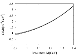
Figure 2: Comparison of the mock data and the OPE data at $\beta=-1$. The solid line shows $G_{\mathrm{OPE}}(M)$ of Eq.(10), with the respective error indicated by the gray region. The dashed line denotes $G_{\mathrm{mock}}(M)$ for which the mock spectral function of Eq.(36) was used.

In order to check the effectiveness of MEM to extract the spectral function of the nucleon, we first carry out an analysis using mock data. The employed mock spectral function is given below:

$$\begin{split}\rho_{\mathrm{mock}}(\omega)=\frac{\lambda^{2}}{2M_{N}^{5}}\delta(\omega-&M_{N})+\frac{5+2\beta+5\beta^{2}}{128(2\pi)^{4}}\frac{1}{1+e^{\frac{(\omega_{0}-\omega)}{\delta}}},\end{split}$$ (36)

$\langle\overline{q}q\rangle$	$\langle\frac{\alpha_{s}}{\pi}G^{2}\rangle$	$\langle\overline{q}g\sigma\cdot Gq\rangle$/$\langle\overline{q}q\rangle$
$-(0.24\pm 0.01)^{3}\,\mathrm{GeV}^{3}$	$0.012\pm 0.0036\,\mathrm{GeV}^{4}$	$0.8\pm 0.2\,\mathrm{GeV}^{2}$

Table 1: Values of the parameters appearing in the OPE, taken from Colangelo .

Figure 3: Spectral functions extracted from $G_{\mathrm{mock}}(M)$ using various default models at $\beta=-1$. The analyzed Borel mass region is 0.91 GeV $\leq$ $M$ $\leq$ 0.97 GeV. The solid line shows $\rho(\omega)$, the dashed line depicts the input mock spectral function and the dash-dotted line stands for the default model. As we explain in Section 3, the three horizontal lines correspond to $\langle\rho_{\mathrm{out}}\rangle+\langle\delta\rho_{\mathrm{out}}\rangle$, $\langle\rho_{\mathrm{out}}\rangle$, $\langle\rho_{\mathrm{out}}\rangle-\langle\delta\rho_{\mathrm{out}}\rangle$, respectively. Similar horizontal lines in following figures are understood to have the same meaning.

where we use the following values for the various parameters:

$$\begin{split}M_{N}&=940\,\mathrm{MeV},\,\omega_{0}=1.3\,\mathrm{GeV},\,\\ \delta&=0.05\,\mathrm{GeV},\,\lambda^{2}=\frac{0.19}{(2\pi)^{4}}\,\mathrm{GeV}^{6}.\end{split}$$ (37)

Here, $\rho_{\mathrm{mock}}(\omega)$ is constructed to have a narrow ground state pole and a continuum, which approaches the perturbative value at high energy. Defining now

$$G_{\mathrm{mock}}(M)\equiv\int^{\infty}_{0}d\omega K(M,\omega)\rho_{\mathrm{mock}}(\omega),$$ (38)

we apply the MEM procedure to

$$G_{\mathrm{mock}}(M)=G_{\rho}(M)=\int^{\infty}_{0}d\omega K(M,\omega)\rho(\omega).$$ (39)

The residue of the nucleon pole $\lambda$ was fitted so that $G_{\mathrm{mock}}(M)$ matches $G_{\mathrm{OPE}}(M)$ at $\beta=-1$ in the analyzed Borel mass region. For comparison, $G_{\mathrm{OPE}}(M)$ and $G_{\rho}(M)$ are shown in Fig. 2. The values of the parameters appearing in Eq.(7) are shown in Table 1. As can be observed in Fig. 2, $G_{\mathrm{OPE}}(M)$ and $G_{\rho}(M)$ are consistent within the range of the error, which shows that the “pole + continuum” ansatz describes the OPE data well. However, this does not necessarily imply that the integral of Eq.(39) can be reliably inverted and that valid information on the nucleon pole can be extracted. To investigate to what extent this is possible, we now analyze $G_{\mathrm{mock}}(M)$. For a realistic analysis, we here employ the error obtained from $G_{\mathrm{OPE}}(M)$, $\sigma_{\mathrm{mock}}(M)=\sigma_{\mathrm{OPE}}(M)$.

To use MEM, we must at first fix the default model $m(\omega)$. A reasonable choice for $m(\omega)$ should reflect our prior knowledge on the spectral function such as the asymptotic behavior at low or high energy. To test several possible choices, we here introduce three types of default models. The first one is a constant consistent only with the asymptotic behavior of the spectral function at low energy, therefore lying close to 0:

$$m_{\mathrm{flat}}(\omega)=1.0\times 10^{-6}.$$ (40)

The detailed value of $m_{\mathrm{flat}}$ is not so important, as long as it can be considered to be small enough compared to the asymptotic value at high energy. As we will discuss in more detail in the section dealing with the gaussian sum rule, we indeed have found that the position of the lowest lying pole and its residue of the obtained spectral functions depend on the value of $m_{\mathrm{flat}}$ only weakly. The second default model is also a constant which now reflects the asymptotic behavior at high energy:

$$m_{\mathrm{asym}}(\omega)=\frac{5+2\beta+5\beta^{2}}{128(2\pi)^{4}}.$$ (41)

The third one is a combination of the first two with the correct behavior at both high and low energy:

$$\begin{split}m_{\mathrm{hybr}}(\omega)&=\frac{5+2\beta+5\beta^{2}}{128(2\pi)^{4}}\frac{1}{1+e^{(\omega_{0}-\omega)/\delta}},\\ \omega_{0}&=1.8\,\mathrm{GeV},\delta=0.1\,\mathrm{GeV}.\end{split}$$ (42)

In the following, the analysis is carried out at $\beta=-1$. In the case of the conventional method, which assumes the spectral function to have a specific functional form such as the “pole + continuum” ansatz, the analyzed Borel mass region is restricted so that the ratio of the highest dimensional term is less than 0.1 of the whole $G_{\mathrm{OPE}}(M)$ to have some confidence on the OPE convergence. The Borel mass region is further limited by the condition that the contribution from the continuum states in $G_{\rho}(M)$ should be less than 0.5 to make sure that the lowest pole dominates the sum rule. The Borel mass region determined according to these restrictions becomes 0.91 GeV $\leq$ $M$ $\leq$ 0.97 GeV. As pointed out in Leinweber2 , this region is very narrow and thus we expect that it will be very difficult to extract $\rho(\omega)$ in a wide range of $\omega$ with this small amount of available information. Although, when using MEM, we can in principle employ values of $M$ above 0.97 GeV, we here first analyze the spectral function using the Borel mass region 0.91 GeV $\leq$ $M$ $\leq$ 0.97 GeV. The results are shown in Fig. 3.

It is clear from Fig. 3, that the obtained lowest peaks lie much above the input value of 940 MeV. Hence, as expected, we cannot extract much information on the nucleon pole from this sum rule. Especially, in the case of the default model $m_{\mathrm{asym}}(\omega)$, the spectral function in the low energy region approaches $m_{\mathrm{asym}}(0)$ and we can only observe a small lowest peak. A similar tendency was observed in the $\rho$-meson channel Gubler1 . We will therefore abandon this default model in the following. In the case of $m_{\mathrm{flat}}(\omega)$, although the high energy behavior wrongly approaches 0 at high energy, the low energy behavior, which is the main focus of our interest, seems to be reasonable. On the other hand, using $m_{\mathrm{hybr}}(\omega)$ leads to the correct behavior at both high and low energy. From these results, we can infer that the default model completely determines the asymptotic values of the spectral function. This behavior at high and low energy should therefore be considered to be an input in the current analysis. This can be understood from the properties of the kernel $K(M,\omega)$, leading to a function $G_{\rho}(M)$, which is insensitive to the values of $\rho(\omega)$ at large and small values of $\omega$. From the behavior of $K(M,\omega)$, we can also expect that increasing the upper boundary of $M$ allows the analysis to become sensitive to $\rho(\omega)$ at higher energy regions.

For investigating this case, we analyze the spectral function under the condition of $M_{\mathrm{min}}$ = 0.91 GeV and $M_{\mathrm{max}}$ = 1.4 GeV. The results are shown in Fig. 4.

Figure 4: Spectral functions extracted from $G_{\mathrm{mock}}(M)$ using various default models at $\beta=-1$. The analyzed Borel mass region is 0.91 GeV $\leq M\leq$ 1.4 GeV. The solid line shows $\rho(\omega)$, the dashed line depicts the input mock spectral function and the dash-dotted line stands for the default model.

When using $m_{\mathrm{flat}}(\omega)$, the resulting spectral function at high energy oscillates around the continuum value before approaching the default model. This is plausible, because the input spectral function has the “pole + continuum” structure, which the MEM analysis is trying to simulate with the given limited information of $G_{\mathrm{mock}}(M)$. Nevertheless, the MEM procedure cannot reproduce the mass of the nucleon, whatever default model or Borel mass range is used.

4.2 Analysis using OPE data

Similar to the previous section, we now carry out the analysis using the real OPE data, $G_{\mathrm{OPE}}(M)$, even though from our experience of the mock data analysis, we cannot expect to obtain meaningful results. We analyze the spectral function by setting the analyzed Borel mass region to 0.91 GeV $\leq M\leq$ 0.97 GeV, as in the last section. The results are shown in Fig. 5. Using a wider Borel mass region leads to spectral functions very similar to the ones shown in Fig. 4. As in the mock data analysis, the MEM procedure does not succeed to reproduce the nucleon peak. The main reason for this failure can be traced back to the slow convergence of the OPE and to the large contribution of continuum to the sum rule. These factors severely reduce the information of the lowest nucleon pole that can be extracted from $G_{\mathrm{OPE}}(M)$.

Figure 5: Spectral functions extracted from $G_{\mathrm{OPE}}(M)$ using various default models at $\beta=-1$. The analyzed Borel mass region is 0.91 GeV $\leq M\leq$ 0.97 GeV. The solid line shows $\rho(\omega)$, the vertical dashed line indicates the position of the nucleon ground state and the dash-dotted line stands for the default model.

5 Analysis using the Gaussian sum rule

In case of the Gaussian sum rule, the analysis is carried out using the following equations:

$$\begin{split}G_{\mathrm{OPE}}(s,\tau)&=G_{\rho}(s,\tau)=\int^{\infty}_{0}d\omega K(s,\tau,\omega)\rho(\omega),\\ K(s,\tau,\omega)&=\frac{2\omega^{5}}{\sqrt{4\pi\tau}}e^{-\frac{(\omega^{2}-s)^{2}}{4\tau}}.\end{split}$$

As before, we set $\beta=-1$ and the results will be shown in terms of the dimensionless spectral function.

5.1 Analysis using mock data

As for the Borel sum rule, we use Eq.(36) as mock data and Eqs.(40 - 42) for the default model. As a first step, we must determine the ranges of s, $\tau$ used in the analysis. From the property of the kernel, we expect that $G_{\mathrm{\rho}}$ at small values of $\tau$ will be more sensitive to narrow structures such as the lowest peak, while $G_{\mathrm{\rho}}$ at larger values will to a large extent be fixed by the continuum. Hence, to extract as much information as possible from $G_{\mathrm{mock}}(s,\tau)$, we use several value of $\tau$ at the same time, which are $\tau$ = 0.5, 1, 1.5, 2$\,\mathrm{GeV}^{4}$. From

$$\lim_{\tau\rightarrow 0}\frac{1}{\sqrt{4\pi\tau}}\mathrm{e}^{-\frac{(\omega^{2}-s)^{2}}{4\tau}}=\delta(\omega^{2}-s),$$ (43)

one understands that in the limit $\tau\to 0$, $G_{\mathrm{\rho}}(s,\tau)$ in principle should approach the spectral function as

$$\lim_{\tau\rightarrow 0}G_{\mathrm{\rho}}(s,\tau)=s^{2}\rho(\sqrt{|s|}).$$ (44)

However, it is not possible to take this limit, because the OPE is an expansion in powers of $1/\sqrt{\tau}$ as can be seen in Eq.(23), meaning that the convergence of the expansion worsens with lower values of $\tau$.

Figure 6: Three examples of the kernel $K(s,\tau,\omega)$. The solid line shows $K(s,\tau,\omega)$ for $s=-0.79\,\mathrm{GeV}^{2}$, the dashed line for $s=0\,\mathrm{GeV}^{2}$ and the dash-dotted line for $s=0.94\,\mathrm{GeV}^{2}$. In all three cases, $\tau$ is fixed to $\tau=0.5\,\mathrm{GeV}^{4}$.

$\tau\,[\mathrm{GeV}^{4}]$	0.5	1	1.5	2
$s_{\mathrm{min}}\,[\mathrm{GeV}^{2}]$	-0.79	-1.84	-2.96	-4.13
$s_{\mathrm{max}}\,[\mathrm{GeV}^{2}]$	0.94	0.02	-0.97	-2.0

Table 2: The analyzed ranges of the variable $s$ for the employed values of $\tau$.

Turning now to the parameter $s$, similar to the Borel sum rule case, we determine its range from the convergence in $G_{\mathrm{OPE}}(s,\tau)$ and the contribution from the continuum in $G_{\rho}(s,\tau)$. The analyzed regions of $s$ and $\tau$ are shown in Table 2. Here, we denote the upper and lower boundaries of $s$ at each $\tau$ as $s_{\mathrm{max}}$ and $s_{\mathrm{min}}$, respectively.

Some further comments are in order here. Firstly, let us briefly explain the method of using the two variables of $s$ and $\tau$ at the same time, compared to the discussion of Section 3, where only one variable $x$ was considered. Generalizing the method from one variable to two is straightforward, as one only needs to redefine the kernel and the likelihood function. Specifically, we use

$$\begin{split}G(x_{i})&=\sum_{\omega_{j}=\omega_{\mathrm{min}}}^{\omega_{\mathrm{max}}}K(x_{i},\omega_{j})\rho(\omega_{j})d\omega\\ &\downarrow\\ G(s_{i},\tau^{k})&=\sum_{\omega_{j}=\omega_{\mathrm{min}}}^{\omega_{\mathrm{max}}}K(s_{i},\tau^{k},\omega_{j})\rho(\omega_{j})d\omega,\end{split}$$

and

$$\begin{split}L(\rho)&=\frac{1}{2(x_{\mathrm{max}}-x_{\mathrm{min}})}\sum^{x_{\mathrm{max}}}_{x_{i}=x_{\mathrm{min}}}dx\frac{[G_{\mathrm{OPE}}(x_{i})-G_{\rho}(x_{i})]^{2}}{\sigma^{2}(x_{i})}\\ &\downarrow\\ L(\rho)&=\sum^{\tau^{\mathrm{max}}}_{\tau^{k}=\tau_{\mathrm{min}}}\sum^{s_{\mathrm{max}}^{k}}_{s_{i}=s_{\mathrm{min}}^{k}}ds^{k}\frac{1}{2(s_{\mathrm{max}}^{k}-s_{\mathrm{min}}^{k})}\\ &\quad\quad\quad\quad\quad\quad\quad\times\frac{[G_{\mathrm{OPE}}(s_{i},\tau^{k})-G_{\rho}(s_{i},\tau^{k})]^{2}}{\sigma^{2}(s_{i},\tau^{k})}.\end{split}$$

In the present analysis, we take 4 data points for $\tau$ ($N_{\tau}=4$), and 25 data points for s ($N_{s}=25$) at each $\tau^{k}$ and adjust $\omega_{\mathrm{min}}$ and $\omega_{\mathrm{max}}$ to 0 and 6 GeV, respectively. $s_{\mathrm{max}}^{k}$ and $s_{\mathrm{min}}^{k}$ at each $\tau^{k}$ are given in Table 2, and $ds^{k}$ is $(s_{\mathrm{max}}^{k}-s_{\mathrm{min}}^{k})/N_{s}$.

Figure 7: Spectral functions extracted from $G_{\mathrm{mock}}(s,\tau)$ using various default models at $\beta=-1$. The analyzed regions of $s$ and $\tau$ are shown in Table 2. The solid line shows $\rho(\omega)$, the dashed line depicts the input mock spectral function and the dash-dotted line stands for the default model.

	mock data	$m_{\mathrm{flat}}$	$m_{\mathrm{hybr}}$	$m_{\mathrm{asym}}$
position of first peak [MeV]	940	1060 $\pm$ 140	1120 $\pm$ 100	1080 $\pm$ 410
position of second peak [MeV]	-	1850	1970	1960
residue of first peak $[10^{-5}\mathrm{GeV}]$	8.3	7.0	6.0	-

Table 3: Position of the peaks and values of the corresponding residues, obtained from a mock data analysis with three default models at $\beta=-1$. Here, the given values of the mock data residue is defined as $\lambda^{2}/(2M_{N}^{5})$. The errors are estimated by evaluating the half width of the obtained first peak.

Secondly, we comment on the ranges of the variable $s$, shown in Table 2. It is seen that to the most part, we use negative values for $s$, which may seem somewhat counterintuitive as, naively, the kernel of Eq.(5) seems to have a peak at $\sqrt{s}$, when considered as a function of $\omega$. Therefore one would expect values of $s$ around 1 GeV to give a $G_{\rho}(s,\tau)$ that is most sensitive to the spectral function in the region of the nucleon pole. However, this is not the case because the kernel is distorted due to the $\omega^{5}$-factor in front of the Gaussian of Eq.(5). For example, for constructing a kernel with a maximum value at 1 GeV which is the energy region which we are mostly interested in, $s$ becomes $1-5\tau$ and, in the case of $\tau=0.5,1,1.5,2$ GeV⁴, has a negative value. This is illustrated in Fig. 6, where one can see that only kernels with negative $s$ have peaks around 1 GeV. From these arguments, we can understand that it is necessary and important to use negative values of $s$ in the analysis of the Gaussian sum rules.

Let us now discuss the obtained spectral functions, which are shown in Fig. 7. Their detailed numerical results are given in Table 3. It is observed that, compared with the Borel sum rule, the reconstruction of the lowest lying peak has considerably improved. Nevertheless, it is seen in Table 3 that its position is shifted upwards about $120\sim 180\,$MeV, which should give an idea of the precision attainable with this method. To evaluate the residue of the first peak, we first have to define the region $\omega$ over which the peak can be considered to be the dominant contribution. The left edge of the first peak is determined to be the point whose height is 1/30 of the peak vertex and the right edge so that the center between the left and the right edge lies on the peak vertex. The residue is then obtained by simply integrating $\rho(\omega)$ over the peak region, indicated by the horizontal length of the error bars. Table 3 shows that the residue of the first peak gives about 80 % of the input value of the mock data. Since the default model $m_{\mathrm{flat}}(\omega)$ leads to a peak position and residue closest to the input values we will use only $m_{\mathrm{flat}}(\omega)$ as the default model in the following.

Here, we comment on the width of the peaks appearing in the obtained spectral functions. One might wonder why these peaks have a finite width even though the input mock data only contains a zero width pole. There are two important aspects related to this point. Firstly, one should note that the OPE side of the sum rule is rather insensitive to the value of the width, because this information is largely lost after the integration over the spectral function in Eqs. (1) or (2). This is so as long as the parameters governing the scales of these integrals ($M$ or $\tau^{1/4}$) are much larger than the width of the peak of interest. This point was discussed explicitly for the $\rho$-meson channel in Gubler1 . Secondly, one should remember that MEM is a statistical method, that can only provide the the most probable form of the spectral function, given the information available. This most likely spectral function depends not only on the input data but also on their error. Generally, a larger error makes a peak broader and smaller in magnitude, therefore introducing an artificial width connected to the error of the OPE data.

Next, to study the dependence of the results on the range of $s$, we fix $s_{\mathrm{max}}$ to 1.0$\,\mathrm{GeV}^{2}$, 1.5$\,\mathrm{GeV}^{2}$ and 2.0$\,\mathrm{GeV}^{2}$ for all values of $\tau$, and redo the analysis. The results are shown in Fig. 8 and Table 4. From Table 4, one can observe that the position and residue of the first peak depends on $s_{\mathrm{max}}$ only weakly, while the position of the second peak is quite sensitive to the value of $s_{\mathrm{max}}$. Furthermore, from the Fig. 8, it can be understood that the second peak rather represents the continuum, around which the MEM output oscillates.

Figure 8: Spectral functions extracted from $G_{\mathrm{mock}}(s,\tau)$ and $m_{\mathrm{flat}}(\omega)$ at $\beta=-1$. Various values of $s_{\mathrm{max}}$ are used as indicated in the figures. The values of $s_{\mathrm{min}}$ at different $\tau$ are shown in Table 2. The solid line shows $\rho(\omega)$ and the dashed line stands for the input mock spectral function.

$s_{\mathrm{max}}\,[\mathrm{GeV}^{2}]$	$s_{\mathrm{max}}=1.0$	$s_{\mathrm{max}}=1.5$	$s_{\mathrm{max}}=2.0$
position of first peak [MeV]	1090 $\pm$ 140	1100 $\pm$ 140	1100 $\pm$ 150
position of second peak [MeV]	1980	2020	-
residue of first peak $[10^{-5}\mathrm{GeV}]$	6.7	6.5	6.3

Table 4: Position of the peaks and values of the corresponding residues. Here, the default model $m_{\mathrm{flat}}(\omega)$ and various $s_{\mathrm{max}}$ values were used. The errors are estimated by evaluating the half width of the obtained first peak.

Finally, we discuss the dependence of the spectral function on the parameters appearing in the default models. In the case of the flat default models as given in Eqs.(40) and (41), we have carried out analyses using several height values (spanning over several orders of magnitude). The results are shown in Fig. 9. It is clear that the detailed values have little influence on the position of the nucleon pole. Extracting the correspoding residues, it is understood that their values also depend on the height value only weakly. Specifically, the pole positions for the curves shown in Fig. 9 coincide within 1% and the residues within 6%. In the case of a hybrid default model as given in Eq.(42), we also carried out analyses using several parameter combinations, the result being that the positions of the obtained first peaks did depend on the parameter combinations only weakly.

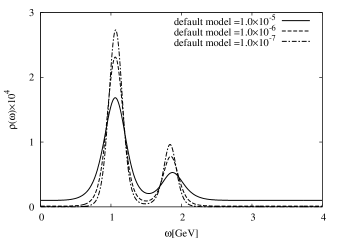
Figure 9: The spectral functions ectracted from $G_{\mathrm{mock}}(s,\tau)$, using various height values for the flat default model $m_{\mathrm{flat}}(\omega)$. The concrete numerical values are given in the figure.

In all, we conclude that using the Gaussian sum rule, reconstruction of the lowest lying peak and the residue of mock data is largely improved compared to the Borel sum rule, and that the attainable precision with the present uncertainties of the condensates is about 20 %.

5.2 Analysis using OPE data

Next, we carry out the analysis using $G_{\mathrm{OPE}}(s,\tau)$. We apply the MEM in the same regions of $s$ and $\tau$ used in the mock data analysis. The results are shown in Fig. 10, while the numerical details are given in Table 5. The behavior of the results is similar to those of the mock data analysis. We observe that the positions of the lowest peak lie quite close to the experimental value. Besides a clearly resolved first peak, the spectral function exhibits one or two higher peaks which oscillate around the asymptotic high energy limit. In principle, this part could also contain nucleon resonances with both positive and negative parity. With the present resolution achievable with the MEM technique, it however seems to be rather difficult to resolve these resonances from the continuum. Using the parity projected sum rules Jido , which can also be analyzed by the MEM approach, might improve the situation.

5.3 Investigation of the $\beta$ dependence

The coupling strengths of the nucleon ground state and its excited states depend on the choice of the interpolating operator, i.e., on the value of $\beta$. To investigate the nature of this dependence, we let $\beta$ vary as $-$1.5, $-$0.5, 0.0, 0.5, 1.0, 1.5, $\infty$ and extract the corresponding spectral functions. For $\tau$, we have chosen 0.5, 1.0, 1.5, 2.0$\,\mathrm{GeV}^{4}$ as before and $s_{\mathrm{min}}$ is determined from the OPE convergence condition at each $\beta$. In the case of $\beta=1$, $s_{\mathrm{min}}$ is determined from the dimension 4 term because the higher dimensional terms vanish for this choice. To obtain information not only on the spectral function around 1 GeV, but also in the region of possible excited states, $s_{\mathrm{max}}$ is not determined from the dominance of the lowest lying state in $G_{\rho}(s,\tau)$ but is fixed to 2.0 GeV². The explicit values of $s_{\mathrm{min}}$ are given in Table 6. Note that $\beta=\infty$ should not be taken literally, but just means that we use the correlator of only $\eta_{2}(x)$ (which is the coefficient of $\beta^{2}$ in Eq.(7)) for the analysis. The resulting spectral functions and their numerical properties are shown in Fig. 11 and Table 7. For a better comparison, we have normalized the spectral functions in Fig. 11 by dividing them by the factor $N(\beta)\equiv(5+2\beta+5\beta^{2})/(128(2\pi)^{4})$, so that the continuum approaches unity in the high energy limit.

Figure 10: Spectral functions extracted from the MEM analysis using $G_{\mathrm{OPE}}(s,\tau)$ and $m_{\mathrm{flat}}(\omega)$ at $\beta=-1$. The solid lines show $\rho(\omega)$ and the dash-dotted lines stands for the asymptotic value of the spectral function at high energy. (Note that $\rho(\omega)$ is normalized by $\frac{1}{\omega^{4}}$.) In the top figure (cont), the values of $s$ and $\tau$ given in Table 2 are used, while for the other figures the values of $s_{\mathrm{max}}$ are fixed as indicated.

$s_{\mathrm{max}}\,[\mathrm{GeV}^{2}]$	$s_{\mathrm{max}}$=(cont)	$s_{\mathrm{max}}$=1.0	$s_{\mathrm{max}}$=1.5	$s_{\mathrm{max}}$=2.0
position of first peak [MeV]	990 $\pm$ 130	1040 $\pm$ 140	1060 $\pm$ 150	1050 $\pm$ 150
position of second peak [MeV]	1840	1920	-	1800
residue of first peak$\,[10^{-5}\mathrm{GeV}]$	7.9	7.0	6.6	6.3

Table 5: Positions of the first and second peaks and the corresponding residues of the first peak obtained from the analyses using OPE data at $\beta=-1$ and the default model $m_{\mathrm{flat}}(\omega)$. The errors are estimated by evaluating the half width of the obtained first peak.

$\beta$	-1.5	-1	-0.5	0	0.5	1	1.5	$\infty$
$\tau=$0.5	-0.40	-0.79	-0.39	-0.35	-0.43	0.92	-0.23	1.04
$\tau=$1.0	-1.21	-1.84	-0.96	-0.87	-1.10	0.12	-0.93	-0.36
$\tau=$1.5	-2.12	-2.96	-1.63	-1.47	-1.87	-0.76	-1.74	-0.88
$\tau=$2.0	-3.07	-4.13	-2.34	-2.13	-2.68	-1.66	-2.60	-1.45

Table 6: Values of $s_{\mathrm{min}}$ [GeV²] at each $\beta$ and $\tau$ [GeV⁴]. $s_{\mathrm{max}}$ is fixed to 2.0 GeV².

Considering first the lowest peaks at $\omega\sim$ 1 GeV, we see that a peak is clearly resolved for $\beta$ = $-$1.0, $-$0.5, 0.0 and 0.5, located at about the same position and with similar residue values. For the other values of $\beta$, no prominent peak is observed. These results are, however, obtained by using the $s_{\mathrm{min}}$ values determined separately for each $\beta$ and one could suspect that the choice of $s_{\mathrm{min}}$ affects the properties of the first peak. To study this dependence and to get an idea of the stability of our results, we redo the analysis, now using values of $s_{\mathrm{min}}$ that are determined via a $\beta$ independent criterion as advocated in Leinweber2 ; Leinweber3 . Taking a closer look at Table 6, it is observed that in the region between $\beta=-1.0$ and $0.5$, where the ground state peak can be extracted, the OPE convergence is worst for $\beta=0.0$, giving the largest value of $s_{\mathrm{min}}$. This implies that it is most reasonable to fix $s_{\mathrm{min}}$ to the values of $\beta=0.0$, so that no values of $s$ are used, where the convergence of the OPE might be questionable. Using this criterion, we repeat the analysis at $\beta$ = $-$1, $-$0.5, 0.5. As before, we set $s_{\mathrm{max}}$ to 2.0 GeV².

Figure 11: Spectral functions obtained from the MEM analyses of OPE data for various values of $\beta$, normalized by the factor $N(\beta)$. The values $s_{\mathrm{min}}$ are given in Table 6 and $s_{\mathrm{max}}$ is fixed to 2.0 GeV².

$\beta$	-1.5	-1	-0.5	0.0	0.5	1	1.5	$\infty$
position of first peak [MeV]	1210	1050	1120	1130	1120	1300	1470	1630
residue of first peak$\,[10^{-5}\mathrm{GeV}]$	-	6.3	5.0	4.8	5.3	-	-	-

Table 7: Positions of the first peaks of the spectral functions shown in Fig. 11. For the cases in which the first peak can be interpreted as the nucleon ground state, the corresponding residue is given as well.

The results are shown and compared to the previous ones in Fig. 12. The numerical details are given in Table 8. We see from these results that some details of the output spectral functions (especially at $\beta=-1$) change when the new criterion is used. The qualitative structure of a clear lowest peak with a continuum structure at a somewhat higher energy is however not altered.

We also observe from Table 8 that the position and residue are almost independent of $\beta$. This fact becomes even more explicit when we plot the non-normalized spectral functions for several values of $\beta$ around $\beta=0$ as shown in Fig. 13. This figure clearly illustrates that, in contrast to the continuum spectra, the property of the lowest peak is essentially $\beta$-independent.

Figure 12: Spectral functions obtained from a MEM analysis of OPE data with $m_{\mathrm{flat}}(\omega)$ at $\beta=-1$, $-0.5$ and $0.5$, normalized by $N(\beta)$. The solid lines show the normalized output spectral function $\rho(\omega)$, for which a $\beta$ independent “refined” criterion was used to determine $s_{\mathrm{min}}$. The details are explained in the text. For comparison, the spectral functions obtained with the previous $\beta$-dependent criterion are indicated by the dashed line.

All these results can be naturally interpreted by presuming that the lowest lying pole couples strongly to $\eta_{1}$, and only very weakly to $\eta_{2}$. Therefore, the pole appears to be almost independent of $\beta$ as long as $|\beta|$ is small, but disappears when $|\beta|$ becomes large and the contribution of $\eta_{2}$ dominates the spectral function. The nucleon ground state pole can be resolved as long as its strength is large enough compared to the continuum contribution. At about $|\beta|\geq 1.5$, however, this continuum contribution gets too large to extract information on the lowest peak. These conclusions agree with the findings of lattice QCD Leinweber3 ; SSasaki ; Melnitchouk and some earlier suggestions of QCD sum rule studies Chung2 , in which however the position of the nucleon ground state peak was used as an input.

Furthermore, by looking at Table 6 and Fig. 12, we can also understand why it is the Ioffe current ($\beta=-1.0$), rather than $\eta_{1}$, that seems to be most suitable for QCD sum rule studies. This comes from the fact that the OPE convergence is considerably faster for the Ioffe compared to $\eta_{1}$, which allows the analysis to become more sensitive to the lower energy region of the spectral function, therefore providing more information on the nucleon peak.

$\beta$	-1	-0.5	0	0.5
position of first peak [MeV]	1120	1120	1130	1140
residue of first peak$\,[10^{-5}\mathrm{GeV}]$	5.3	4.9	4.8	5.1

Table 8: Positions of the first peaks and the corresponding residues of the spectral functions shown in Fig. 12, where a $\beta$-independent criterion was used to fix $s_{\mathrm{min}}$. For comparison, the result for $\beta$=0 is shown as well.

Figure 13: Non-normalized spectral functions obtained from a MEM analysis using OPE data and $m_{\mathrm{flat}}(\omega)$ at $\beta$ = $-$1.0, $-$0.5, 0, 0.5. The employed $s_{\mathrm{min}}$ is fixed to the one at $\beta=0$ and $s_{\mathrm{max}}$ to 2.0 GeV².

As a last point, let us also consider the continuous structure above the nucleon ground state pole and possible excited states appearing there. It can be observed in Fig. 11 that for most values of $\beta$, the spectral function just oscillates around the high energy limit, similar to the results obtained from the mock data analysis shown in Fig. 8, where we have only included the continuum and no resonances into the input spectral function. On the other hand, for $\beta=1.5$ and especially $\beta=\infty$, the behavior is somewhat different, showing a quite clear first peak at about 1.6 GeV. This peak could correspond to one of the nucleon resonances, N(1440), N(1535), N(1650) or a combination of them. Results of lattice QCD studies SSasaki ; Melnitchouk indicate that $\eta_{2}$ couples to the negative parity states N(1535) and N(1650), while the first excited positive parity state lies considerably above the Roper resonance N(1440). Even though the systematic uncertainties of these calculations are probably not yet completely under control, these findings suggest that the lowest peak seen at $\beta=\infty$ corresponds rather to N(1535) or N(1650) and not to N(1440). It, however, seems to be difficult at the present stage to make any conclusive statements on the nature of this peak. An analysis of the parity projected sum rules will hopefully help to clarify this issue.

6 Summary and Conclusion

In this study, we have applied the MEM technique, which is based on Bayes’ theorem of probability theory to the analysis of the nucleon QCD sum rules. We have investigated two kinds of sum rules, namely the frequently used Borel sum rule and the less known Gaussian sum rule. Before analyzing the actual sum rules, we have first tested the applicability of the MEM approach by constructing and analyzing realistic mock data. Our findings show that due to the properties of the kernel and the slow OPE convergence, it appears to be difficult to extract much meaningful information on the nucleon ground state from the Borel sum rule. Another reason for this failure may also be that, because only spectral functions satisfying positivity can be analyzed with the currently available MEM procedure, we cannot use the chiral odd part $\Pi_{2}(q^{2})$ of Eq.(6) in the present analysis, which has been claimed to be more reliable. For instance, in Leinweber2 analyses using only $\Pi_{1}(q^{2})$ or $\Pi_{2}(q^{2})$ were carried out and the respective Borel windows examined. As a result, in case of only using $\Pi_{1}(q^{2})$, the Borel window is seen to be very narrow, making it difficult to obtain a reliable estimate for the nucleon mass. On the other hand, in case of using only $\Pi_{2}(q^{2})$, the borel window was shown to be sufficiently large, so that the nucleon mass can be reliably obtained. It therefore would be helpful if $\Pi_{2}(q^{2})$ could be used. As long as one uses MEM, this, however, will only become possible when the parity projected sum rules are employed. As an alternative, we have formulated the Gaussian sum rule and found that it allows us to extract more information on the spectral function and enables us to reconstruct the nucleon ground state with reasonable precision from both the mock and the OPE data.

As the analysis is done with the MEM technique, we obtain the spectral function directly and do not have to deal with quantities depending on unphysical parameters such as the Borel mass. Moreover, we do not have to restrict the spectral function to the traditional “pole + continuum” form, which allows us to investigate the spectral function of a large variety of of interpolating fields. From this investigation, we have found that the nucleon pole is independent of the parameter $\beta$ of Eq.(5) and vanishes when $\eta_{2}$ becomes the dominant contribution of the correlator. Thus we conclude that, in agreement with findings of lattice QCD, the nucleon ground state couples only to the interpolating field $\eta_{1}$, but not (or only very weakly) to $\eta_{2}$. Furthermore, a peak structure is seen around 1.6 GeV in the spectral function corresponding to $\eta_{2}$, which suggests that some nucleon resonance in this region couples to $\eta_{2}$. To clarify the nature of this peak, more thorough investigations are needed.

In all, we have shown that the MEM technique in combination with the Gaussian sum rule formulated in this paper is useful for extracting the properties of the nucleon ground state and may even make it possible to investigate possible excited states. There are, however, still several open questions to be answered. First of all, we have so far ignored all radiative $\alpha_{s}$ corrections to the Wilson coefficients. These corrections are known to be significant and it is therefore important to include them for a more quantitative analysis. Additionally, possible violations of the vacuum saturation approximation should also be considered. As a further point, it would be crucial to separate the contributions from positive and negative parity states to the spectral function, especially to investigate the excited nucleon resonances. These issues are left for future investigations.

- (1) M.A. Shifman, A.I. Vainshtein, and V.I. Zakharov, Nucl. Phys. B147, 385 (1979); B147, 448 (1979).
- (2) B.L. Ioffe, Nucl. Phys. B188, 317 (1981); B191, 591(E) (1981).
- (3) N.V. Krasnikov, A.A. Pivovarov and N.N. Tavkhelidze, Z. Phys. C 19, 301 (1983).
- (4) Y. Chung, H.G. Dosch, M. Kremer and D. Schall, Z. Phys. C 25, 151 (1984).
- (5) M. Jamin, Z. Phys. C 37, 635 (1988).
- (6) A.A. Ovchinnikov, A.A. Pivovarov and L.R. Surguladze, Int. J. Mod. Phys. A 6, 2025 (1991).
- (7) H. Shiomi and T. Hatsuda, Nucl. Phys. A594, 294 (1995).
- (8) V.A. Sadovnikova, E.G. Drukarev and M.G. Ryskin, Phys. Rev. D 72, 114015 (2005).
- (9) V.M. Belyaev and B.L. Ioffe, Sov. Phys. JETP 56, 493 (1983).
- (10) D.B. Leinweber, Ann. Phys. (N.Y.) 198, 203 (1990).
- (11) K.C. Yang, W.Y.P. Hwang, E.M. Henley and L.S. Kisslinger, Phys. Rev. D 47, 3001 (1993).
- (12) D.B. Leinweber, Ann. Phys. (N.Y.) 254, 328 (1997).
- (13) T. Hatsuda, H. Hogaasen and M. Prakash, Phys. Rev. Lett. 66, 2851 (1991).
- (14) T.D. Cohen, R.J. Furnstahl, D.K. Griegel and X. Jin, Prog. Part. Nucl. Phys. 35 221 (1995).
- (15) E. G. Drukarev, M. G. Ryskin and V. A. Sadovnikova, arXiv:1012.0394 [nucl-th].
- (16) C. Adami and I. Zahed, Phys. Rev. D 45, 4312 (1992).
- (17) P. Gubler and M. Oka, Prog. Theor. Phys. 124, 995 (2010).
- (18) P. Gubler, K. Morita and M. Oka, Phys. Rev. Lett. 107, 092003 (2011).
- (19) R.A. Bertlmann, G. Launer and E. de Rafael, Nucl. Phys. B250, 61 (1985).
- (20) G. Orlandini, T.G. Steele and D. Harnett, Nucl. Phys. A686, 261 (2001).
- (21) V.D. Efros, W. Leidemann and G. Orlandini, Phys. Lett. B338, 130 (1994).
- (22) V.D. Efros, W. Leidemann, G. Orlandini and N. Barnea, J. Phys. G: Nucl. Part. Phys. 34, R459 (2007).
- (23) Y. Chung, H.G. Dosch, M. Kremer and D. Schall, Nucl. Phys. B 197 (1982) 55.
- (24) Y. Chung, H.G. Dosch, M. Kremer and D. Schall, Z. Phys. C 15, 367 (1982).
- (25) B.L. Ioffe, Z. Phys. C 18 (1983) 67.
- (26) H.G. Dosch, M. Jamin and S. Narison, Phys. Lett. B 220, 251 (1989).
- (27) M. Asakawa, T. Hatsuda, and Y. Nakahara, Prog. Part. Nucl. Phys. 46, 459 (2001).
- (28) R.K. Bryan, Eur. Biophys. J. 18, 165 (1990).
- (29) M. Jarrel and J.E. Gubernatis, Phys. Rep. 269, 133 (1996).
- (30) K. Sasaki, S. Sasaki and T. Hatsuda, Phys. Lett. B623 208, (2005).
- (31) P. Colangelo and A. Khodjamirian, “At the Frontier of Particle Physics/Handbook of QCD” (World Scientific, Singapore, 2001), Volume 3, 1495.
- (32) D. Jido, N. Kodama and M. Oka, Phys. Rev. D 54, 4532 (1996).
- (33) D.B. Leinweber, Phys, Rev. D 51, 6383 (1995).
- (34) S. Sasaki, T. Blum and S. Ohta, Phys. Rev. D 65, 074503 (2002).
- (35) W. Melnitchouk et al., Phys. Rev. D 67, 114506 (2003).