Spontaneous symmetry breaking in Schrödinger lattices with two nonlinear sites

Abstract

We introduce discrete systems in the form of straight (infinite) and ring-shaped chains, with two symmetrically placed nonlinear sites. The systems can be implemented in nonlinear optics (as waveguiding arrays) and BEC (by means of an optical lattice). A full set of exact analytical solutions for symmetric, asymmetric, and antisymmetric localized modes is found, and their stability is investigated in a numerical form. The symmetry-breaking bifurcation (SBB), through which the asymmetric modes emerge from the symmetric ones, is found to be of the subcritical type. It is transformed into a supercritical bifurcation if the nonlinearity is localized in relatively broad domains around two central sites, and also in the ring of a small size, i.e., in effectively nonlocal settings. The family of antisymmetric modes does not undergo bifurcations, and features both stable and unstable portions. The evolution of unstable localized modes is investigated by means of direct simulations. In particular, unstable asymmetric states, which exist in the case of the subcritical bifurcation, give rise to breathers oscillating between the nonlinear sites, thus restoring an effective dynamical symmetry between them.

I Introduction

Spontaneous symmetry breaking is a fundamental effect caused by the interplay of nonlinearity with linear potentials featuring basic symmetries, such as double-well structures. In particular, while it is commonly known that the ground state in one-dimensional quantum mechanics follows the symmetry of the underlying double-well potential LL , the self-attractive nonlinearity added to the respective Schrödinger equation [which transforms it into the Gross-Pitaevskii equation for a Bose-Einstein condensate (BEC) of interacting atoms loaded into the double-well potential BEC , or into the nonlinear Schrödinger equation in optical counterparts of the system NLS ] breaks the symmetry of the ground state, replacing it by a new asymmetric state minimizing the system’s energy, provided that the strength of the self-attraction exceeds a certain critical value (see, e.g., Ref. misc for the general consideration, and Ref. misc2 for the analysis of the symmetry-breaking self-trapping in BEC). The spontaneous symmetry breaking in double-well potentials was realized experimentally in BEC Markus and in nonlinear optics, where the symmetry breaking was observed in a setup based on a photorefractive material photo .

The symmetry-breaking bifurcation (SBB), which destabilizes the symmetric ground state and gives rise to an asymmetric one in the nonlinear system, was originally discovered in a discrete model of self-trapping Chris . In nonlinear optics, a similar SBB was predicted in Ref. Snyder for continuous-wave (spatially uniform) states in the model of dual-core fibers. For solitons in dual-core systems, this bifurcation was studied in detail in Ref. dual-core . Subsequently, the SBB was studied for gap solitons in dual-core fiber Bragg gratings with the same Kerr (cubic) nonlinearity as in the ordinary fibers Mak . In another physical setting which also features the cubic nonlinearity, the SBB was predicted for matter-wave solitons in the self-attractive BEC loaded into a dual-trough potential trap Arik -Luca .

The self-focusing cubic nonlinearity gives rise to the soliton bifurcations of the subcritical (alias backward) type, in which the branches of asymmetric modes emerge as unstable ones, going backward and getting stabilized after switching their direction forward at turning points bif . On the other hand, the combination of the self-focusing nonlinearity with a periodic potential acting in the free direction (perpendicular to the direction of the action of the double-well potential) changes the character of the bifurcation from subcritical to supercritical, with the asymmetric branches emerging as stable ones and immediately going in the forward direction Arik ; Warsaw2 . The SBB in the model of the dual-core fiber Bragg grating is of the forward type too Mak . The sub- and supercritical (alias backward/forward) SBBs may be regarded as examples of phase transitions of the first and second kinds, respectively bif .

A physically interesting alternative to the linear double-well potential is the setting with an effective pseudopotential Harrison induced by the double-peak spatial modulation of the local nonlinearity coefficient, which may be implemented in optics and BEC alike Pu ; Barcelona . The ultimate form of such a setting is the one with the nonlinearity concentrated at two points, in the form of a symmetric pair of delta-functions or narrow Gaussians Thawatchai ; Nir , as well as a two-dimensional counterpart of the system, in the form of two parallel troughs in which the nonlinearity is applied Hung (the underlying model, with the self-attractive nonlinearity represented by a single delta-function, was introduced much earlier in Ref. Mark ). The SBB of solitons in the symmetric double-well nonlinear pseudopotentials was studied recently, featuring the subcritical type of the symmetry breaking Thawatchai ; Hung ; Nir .

The spontaneous symmetry breaking was also analyzed for solitons in dual-core discrete systems, with the uniform coupling between two parallel chains Herring , or with the coupling established at a single site Ljupco . In the former case, the SBB is subcritical, while in the latter case it is supercritical.

The objective of the present work is to consider the SBB in one-dimensional discrete lattices with the nonlinearity tightly concentrated at two symmetric sites, or in narrow regions around them. This is a straightforward discrete counterpart of the double-well nonlinear pseudopotential Thawatchai ; Nir , which offers a simple testbed for the study of symmetry-breaking effects in discrete media. Physically, the linear chain with two nonlinear sites can be readily implemented in optics, by embedding two nonlinear cores into an arrayed linear waveguide, and in BEC, by means of the Feshbach-resonance technique applied locally to the condensate trapped in a deep optical lattice BEC . An essential advantage of the system is that, as we demonstrate below, it admits a fully analytical solution (for the infinite chain), with an arbitrary separation between the two symmetric nonlinear sites, while the stability of the exact solutions may be efficiently predicted following general principles of the elementary bifurcation theory bif and the Vakhitov-Kolokolov (VK) criterion VK .

The paper is organized as follows. The model is introduced in Section 2, which is followed by producing exact solutions for symmetric, asymmetric, and antisymmetric localized modes in Section 3. Numerical results, obtained for finite lattices, are reported in Section 4 (in particular, it is demonstrated that the SBB is subcritical in the system with two nonlinear sites). In Section 5, we consider an essentially different version of the system, in the form of a ring-shaped chain, with the two nonlinear sites placed at diametrically opposite points, in which case an analytical solution for the SBB is available too. The paper is concluded by Section 6.

II The model

According to what is said above, the model is based on the linear discrete Schrödinger equation with two nonlinear sites embedded into it:

$$i\frac{du_{n}}{dt}+(1/2)\left(u_{n+1}+u_{n-1}-2u_{n}\right)+\left(\delta_{n,0}+\delta_{n,l}\right)\left|u_{n}\right|^{2}u_{n}=0,$$ (1)

where $l$ is the integer distance between the two nonlinear sites, and $\delta_{n,m}$ is the Kronecker’s symbol. The evolutional variable, $t$, is time in the application to BEC, or propagation distance in the case of an array of optical waveguides. In the former case, the nonlinearity at two sites can be induced by focusing laser beams, that may enhance the nonlinearity through the Feshbach resonance optical-FR , at two particular droplets of the condensate trapped in a deep optical lattice. In the photonic realization of the setting, strong nonlinearity in two particular cores in the waveguiding array can be readily imposed by doping them with resonant atoms (see, e.g., Ref. doping ), which does not affect the linear coupling of these sites to adjacent ones, as implied in Eq. (1). The same mechanisms can be used for inducing the local nonlinearity in circular configurations considered below in Section 5.

Stationary solutions to Eq. (1) are sought for as $u_{n}(t)=e^{-i\omega t}U_{n}$, where real stationary field $U_{n}$ obeys equation

$$\omega U_{n}+(1/2)\left(U_{n+1}+U_{n-1}-2U_{n}\right)+\left(\delta_{n,0}+\delta_{n,l}\right)U_{n}^{3}=0.$$ (2)

Along with this model, we will also consider its version with a smoothed form of the discrete delta-function, viz.,

$$\delta_{n,n_{0}}\rightarrow\exp\left(-\left(n-n_{0}\right)^{2}/\Delta^{2}\right),$$ (3)

where $n_{0}=0$ or $l$, and $\Delta$ is the smoothing width.

A preliminary remark is that Eq. (2) with $l=0$ corresponds to the single nonlinear site with the double strength, placed at $n=0$. In that case, an obvious exact solution is

$$\left(U_{n}\right)_{\mathrm{single}}=Ae^{-\kappa|n|},~{}A^{2}=(1/2)\sinh\kappa\text{,}$$ (4)

where $\kappa$ is connected to $\omega$ by the dispersion relation for evanescent waves in the linear lattice:

$$\omega=-2\sinh^{2}\left(\kappa/2\right).$$ (5)

Taking relation (5) into regard, the norm of solution (4) is

$$N\equiv\sum_{n=-\infty}^{+\infty}U_{n}^{2}=(1/2)\cosh\kappa\equiv\left(1-\omega\right)/2.$$ (6)

Note that this expression for $N$ satisfies the VK stability criterion, $dN/d\omega<0$, hence solutions (4) may be stable MIW . On the other hand, the continuous counterpart of Eq. (2) with the single nonlinear site is

$$\omega U+\frac{1}{2}\frac{d^{2}U}{dx^{2}}+2\delta(x)U^{3}=0,$$ (7)

where $\delta(x)$ is the delta-function (this continuous equation was first introduced in Ref. Mark ). It has an obvious localized solution,

$$U(x)=\left(-\omega/2\right)^{1/4}\exp\left(-\sqrt{-2\omega}|x|\right),$$ (8)

whose norm is degenerate (it does not depend on $\omega$): $N\equiv\int_{-\infty}^{+\infty}U^{2}(x)dx=1/2$. Being formally neutrally stable in terms of the VK criterion, all solutions (8) are actually unstable Nir . The degeneracy and instability of solutions (8) resemble the classical properties of the Townes’ solitons Townes .

III Exact solutions for the infinite lattice

III.1 General analysis

Symmetric, antisymmetric, and asymmetric solutions to Eq. (2) can be found in an exact form, following the pattern of the exact solutions for the continuous counterpart of Eq. (2), which was considered in Ref. Thawatchai :

$$\omega U+\frac{1}{2}\frac{d^{2}U}{dx^{2}}+\left[\delta\left(x\right)+\delta\left(x-l\right)\right]U^{3}=0,$$ (9)

cf. Eq. (7). Exact symmetric and asymmetric solutions to the discrete equation (2) are sought in the following form:

$$U_{n}=\left\{\begin{array}[]{cc}Ae^{\kappa n},&\mathrm{at}~{}~{}n\leq 0,\\ B\cosh\left(\kappa\left(n-n_{0}\right)\right),&\mathrm{at}~{}0\leq n\leq l,\\ Ce^{-\kappa\left(n-l\right)},&\mathrm{at}~{}n\geq l.\end{array}\right.$$ (10)

Coordinate $n_{0}$ determines the location of the center of the intermediate part of the solution. Note that $n_{0}$ does not need to be an integer number. Symmetric and asymmetric modes correspond, respectively, to $n_{0}=l/2$ and $n_{0}\neq l/2$.

Ansatz (10) automatically satisfies the linear discrete Schrödinger equation. There remains to check Eq. (2) at the nonlinear sites (of course, imposing the condition of the continuity of the solution at these sites). With regard to Eq. (5), the continuity condition yields relations between the amplitudes:

$$B=\frac{A}{\cosh\left(\kappa n_{0}\right)}=\frac{C}{\cosh\left(\kappa l-\kappa n_{0}\right)}~{},$$ (11)

and the equation at the nonlinear sites amounts to the following relations:

$$A^{2}=\frac{\sinh\kappa}{1+e^{-2\kappa n_{0}}},~{}C^{2}=\frac{\sinh\kappa}{1+e^{-2\kappa\left(l+n_{0}\right)}}.$$ (12)

After some algebra, the condition that Eqs. (11) and (12) yield the same expression for $B$ produces an equation for $n_{0}$:

$$x^{4}+\left(3-L\right)x^{3}+\left(1-3L^{-1}\right)x-L^{-2}=0,$$ (13)

$$x\equiv e^{-2\kappa n_{0}},~{}L\equiv e^{2\kappa l}.$$ (14)

III.2 Symmetric modes

Two roots of quartic equation (13) are $x=\pm L^{-1/2}$. The negative one is unphysical, while the positive root corresponds, according to Eq. (14), to $n_{0}=l/2$, which represents the symmetric mode. The amplitudes of the symmetric solution, as given by Eqs. (11) and (12), are

$$A^{2} = C^{2}=\frac{\sinh\kappa}{1+e^{-\kappa l}},$$ (15a)

$$B^{2} = \frac{4e^{-\kappa l}\sinh\kappa}{\left(1+e^{-\kappa l}\right)^{3}}~{}.$$ (15b)

It is relevant to note that, in the case of $$l=0 A^{2}=B^{2}=C^{2}=(1/2)\sinh\kappa A^{2}$$, Eqs. (15) yield , which naturally coincides with as given by Eq. (4).

III.3 Asymmetric modes

Two other roots of Eq. (13) represent a pair of asymmetric modes:

$$x_{\pm}=\frac{1}{2}\left[\left(L-3\right)\pm\left(L-1\right)\sqrt{\frac{L-4}{L}}\right].$$ (16)

Taking into regard Eq. (14), it is easy to check that roots (16) correspond to two values $\left(n_{0}\right)_{\pm}$ which are located mutually symmetrically around the center: $x_{+}x_{-}=L^{-1}$, i.e., $\left(n_{0}\right)_{+}+\left(n_{0}\right)_{-}=l$. Further, roots (16) are physical if they are real and positive, which means $L>4$. Thus, the symmetry-breaking bifurcation (SBB), i.e., the appearance of the asymmetric modes from the symmetric one [see Fig. 1(a)], happens, with the increase of distance $l$ between the nonlinear sites (at fixed $\kappa$, i.e., fixed $\omega$), at the critical point, $\kappa_{\mathrm{cr}}l=\ln 2$, or, in terms of the frequency of the localized mode, at

$$\omega=\omega_{\mathrm{cr}}^{-}=-2\sinh^{2}\left(\frac{\ln 2}{2l}\right).$$ (17)

In other words, for fixed $l$, the SBB occurs with the increase of $\left|\omega\right|$ at point (17), the asymmetric modes existing at $\left|\omega\right|>\left|\omega_{\mathrm{cr}}^{-}\right|$.

The asymmetric mode keeps the double-peak shape if the minimum point in expression (10), $n_{0}$, is a really existing minimum, rather than a virtual one, i.e., it stays in interval $0<n_{0}<l$. Further, this means that $x_{\pm}$ must fall into the following interval: $L^{-1}<x_{\pm}<1$. It is easy to check, making use of Eq. (16), that the latter condition places $L$ and $l$ into narrow intervals of their values, namely, $4<L<2+\sqrt{5}\approx 4.24$, and, accordingly,

$$\ln 2\approx 0.69<\kappa l<(1/2)\ln\left(2+\sqrt{5}\right)\approx 0.72,$$ (18)

cf. Eq. (17). At $\kappa l>\left(1/2\right)\ln\left(2+\sqrt{5}\right)$, i.e., $\omega<\omega_{\mathrm{cr}}^{+}=-2\sinh^{2}\left[\left(4l\right)^{-1}\ln\left(2+\sqrt{5}\right)\right]$ [in other words, at $|\omega|>\left|\omega_{\mathrm{cr}}^{+}\right|$, cf. Eq. (17)], $n_{0}$ leaves the region of $0<n_{0}<l$, hence the asymmetric mode becomes single-peaked (“strongly asymmetric”). The transition from the double-peak asymmetric mode to the single-peak shape is illustrated by Fig. 3(b).

The final expressions for the amplitudes of the asymmetric mode are obtained by the substitution of expressions (16) and (14) into Eqs. (11) and (12):

$$\left\{A^{2},C^{2}\right\}=\left\{\frac{2e^{\kappa l}\sinh\kappa}{\left(e^{2\kappa l}-1\right)\left(e^{\kappa l}\pm\sqrt{e^{2\kappa l}-4}\right)}\right\}$$ (19a)

$$B^{2}=\frac{16e^{2\kappa l}\left[e^{\kappa l}\left(e^{2\kappa l}-3\right)\pm\left(e^{2\kappa l}-1\right)\sqrt{e^{2\kappa l}-4}\right]\sinh\kappa}{\left(e^{2\kappa l}-1\right)^{3}\left(e^{\kappa l}\pm\sqrt{e^{2\kappa l}-4}\right)^{3}}.$$ (19b)

where signs $$\pm e^{\kappa l}=2 A^{2}=C^{2}=\left(2/3\right)\sinh\kappa B^{2}=\left(16/27\right)\sinh\kappa$$ pertain to the two conjugate asymmetric modes. Note that, at the SBB point, , expressions (19) coincide with their counterparts (15) obtained above for the symmetric mode: at this point, the amplitudes are and .

As a natural measure of their asymmetry, we will use

$$\Theta\equiv\frac{A^{2}-C^{2}}{A^{2}+C^{2}}=\pm\sqrt{1-4e^{-2\kappa l}}.$$ (20)

Obviously, $\Theta=0$ at the SBB point, $e^{-\kappa l}=1/2$, and expression (20) makes sense past the bifurcation point, i.e., at $e^{-\kappa l}<1/2$. In particular, at the above-mentioned point of the transition from the double- to single-peak profile, $\kappa l=\left(1/2\right)\ln\left(2+\sqrt{5}\right)$, the asymmetry is still relatively small, $\left|\Theta\right|=\sqrt{5}-2\approx\allowbreak 0.24$.

III.4 Antisymmetric modes

Antisymmetric solutions, and their counterparts with broken antisymmetry (if any) are looked for by dint of the following ansatz, cf. Eq. (10):

$$U_{n}=\left\{\begin{array}[]{cc}Ae^{\kappa n},&\mathrm{at}~{}~{}n\leq 0,\\ B\sinh\left(\kappa\left(n-n_{0}\right)\right),&\mathrm{at}~{}0\leq n\leq l,\\ U_{n}=Ce^{-\kappa\left(n-l\right)},&\mathrm{at}~{}n\geq l.\end{array}\right.$$ (21)

Looking for a bifurcation occurring to the antisymmetric mode, one arrives at the respective roots for $x$ [with $x$ defined as in Eq. (14)]:

$$x_{\pm}=\frac{1}{2}\left[-\left(L-3\right)\pm\left(L-1\right)\sqrt{\frac{L-4}{L}}\right],$$ (22)

which differs from Eq. (16) by the opposite sign in front of the first term in the square brackets. This difference makes both roots (22) negative (unphysical), hence the antisymmetric solutions do not undergo the bifurcation, similar to the situation known in the continuous model (Thawatchai ).

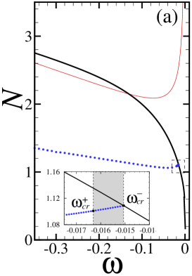
Figure 1: (Color online) (a) The bifurcation diagram in the plane of the intrinsic frequency of the localized modes ($\omega$) and their total norm ($N$), as produced by the analytical solution for the infinite lattice with two symmetric nonlinear sites, separated by distance $l=4$. The black thick, red thin and blue dotted lines correspond to the symmetric (15), antisymmetric (23) and asymmetric (19) solutions, respectively. In the insert, the zoom of the bifurcation of the branch of asymmetric solutions (the blue dotted line) is shown. The gray area determines the region of the existence of the two-peaked asymmetric solution, limited by critical frequencies $\omega_{\mathrm{cr}}^{+}<\omega<\omega_{\mathrm{cr}}^{-}$. In panels (b)-(d), examples of analytically found symmetric, antisymmetric and asymmetric modes at $\omega=-0.016$ and $l=4$ are shown.

The mode with the unbroken antisymmetry is given by the exact solution in the form of ansatz (21) with amplitudes

$$A=-C=\sqrt{\frac{\sinh\kappa}{1-e^{-\kappa l}}},$$ (23a)

$$B=-\frac{2\sqrt{\sinh\kappa}e^{-\kappa l/2}}{\left(1-e^{-\kappa l}\right)^{3/2}}.$$ (23b)

Finally, it is natural to call the antisymmetric modes, corresponding to even and odd $$l n_{0}=l/2$$, on-site and inter-site ones, respectively, as they have the zero point, , either coinciding or not with the (central) site of the lattice.

IV Numerical results for a finite lattice

The objective of the numerical solution is to obtain solutions of stationary equation (2) for a finite lattice, compare them to the exact solutions found above for the infinite lattice and identify stability of the symmetric, asymmetric and antisymmetric solutions. In addition, the numerical calculations help to identify the type of the SBB (sub- or supercritical), as the analytical solution produces a very cumbersome result, in this respect. Numerical stationary solutions were constructed in the lattice of 71 sites. Highly asymmetric modes were obtained by means of the continuation in $\omega$, using the Newton’s iteration procedure that started from the analytical asymmetric solution given by Eqs. (10) and (19). For all numerical solutions, we analyzed the linear stability by solving the corresponding linear eigenvalue problem. The results were checked by direct simulations of the underlying equation (1).

IV.1 Symmetric modes

In Fig. 2, families of numerically generated symmetric solutions are shown for different distances ($l$) between the two nonlinear sites. As said above, the stability of the numerically found solutions was identified through the calculation of the corresponding eigenvalues of small perturbations. The borders between stable and unstable segments of the solution branches correspond to the SBB which destabilizes the symmetric solutions. The numerical solutions are practically indistinguishable from their analytical counterparts (10), (15), therefore the analytically found curves are not plotted separately (strictly speaking, the numerical results cannot be identical to the analytical ones, as the numerical computations were performed for the finite chain, while the analytical findings pertain to the infinite one).

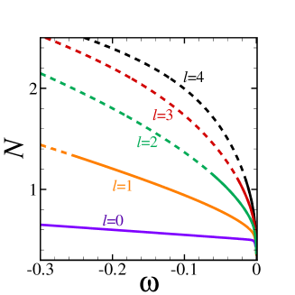
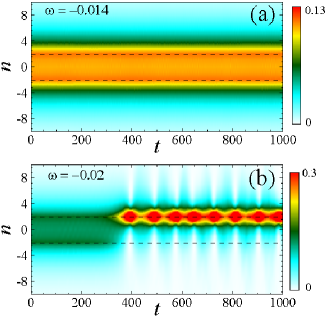
Figure 2: (Color online) Left panel: Families of numerically generated symmetric solutions (their analytical counterparts are indistinguishable from the numerical ones). The corresponding values of the distance between the nonlinear sites, $l$, are indicated. The solid and dashed lines depict, respectively, stable and unstable portions of the solution families. Right panel: The evolution of stable (a) and unstable (b) symmetric modes with $l=4$, taken at $\omega=-0.014$ and $\omega=-0.02$, respectively. Here and in similar plots below, the spatiotemporal evolution is displayed by means of the density contour plots. Small perturbations ($\sim 1\%$) were added to initiate the evolution. Dashed lines show the position of nonlinear sites.

To check the predictions of the linear stability analysis, we simulated the underlying equation (1), with initial profiles for symmetric modes taken in regions where these solutions are expected to have different stability. Typical examples, presented in right panel of Fig. 2, show that the unstable symmetric stationary solution transforms into a pulsating single-peak mode, which breaks the symmetry, getting spontaneously localized on one of the nonlinear sites.

IV.2 Asymmetric modes

The numerical results for the asymmetric modes are displayed in Fig. 3(a). In particular, unstable parts of the families of asymmetric solutions are those which are related to the SBB of the subcritical type [see Fig. 4(b) below]. The SBB displayed by the numerical results closely follows the analytical solution for the infinite lattice. In particular, generic numerically found profiles of the double-peaked (above $\omega_{\mathrm{cr}}^{+}$) and single-peak (below $\omega_{\mathrm{cr}}^{+}$) asymmetric modes are compared with their analytical counterparts in Fig. 3(b), the difference between the numerical and analytical solutions being $\lesssim 1\%$.

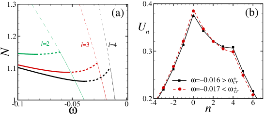
Figure 3: (Color online) (a): The bold and thin lines show, respectively, the families of asymmetric and symmetric solutions. As in Fig. 2, solid and dashed lines corresponds to stable and unstable portions of the solution families. In fact, the lines for the symmetric solutions are identical to those displayed in Fig. 2. (b): An example of the transition from the double-peak shape for $\omega>\omega_{cr}^{+}$ to the single-peak one for $\omega<\omega_{cr}^{+}$, obtained from numerical (circles and squares) and analytical (red dashed and black solid lines) solutions.

In Fig. 4 the numerical results obtained for the asymmetric solutions are collected in the form of plots showing the asymmetry measure defined, as per Eq. (20), through the difference between squared amplitudes of the solution at the two nonlinear sites, as a function of frequency $\omega$ and total norm $N$. The corresponding discrepancy between the numerical and analytical results is $<1\%$. In panel (a), the numerically found bifurcation points are compared to those predicted analytically by Eq. (17) (they correspond to values of $\omega_{\mathrm{cr}}^{-}$ indicated in the panel), which demonstrates a precise agreement. An important conclusion clearly suggested by Fig. 4(b) is that the bifurcation has the subcritical character, with the asymmetric branches being unstable exactly between the SBB and turning points, as might be expected.

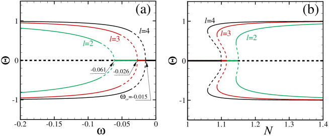
Figure 4: (Color online) The family of the numerically found asymmetric solutions in the planes of $(\Theta,\omega)$ (a) and $(\Theta,N)$ (b) for different distances between the nonlinear sites ($l$). As above, the stable and unstable portions of the solution families are depicted by solid and dashed lines, respectively.

To check the predictions of the linear-stability analysis, we simulated the underlying equation (1) with initial profiles for asymmetric modes taken in the regions where these solutions are expected to be stable and unstable, respectively. Typical examples, presented in Fig. 5, show that the unstable asymmetric stationary solution transforms itself, after a transient period, into a robust breather oscillating between two asymmetric configurations (in that sense, the breathers restores an effective dynamical symmetry).

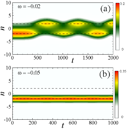
Figure 5: ((Color online) The evolution of unstable (a) and stable (b) asymmetric modes with $l=4$, taken at $\omega=-0.02$ and $\omega=-0.05$, respectively. Dashed lines show the position of nonlinear sites.

IV.3 Antisymmetric modes

Families of numerically found on-site (a) and inter-site (b) antisymmetric modes are shown in Fig. 6. As in the previous cases the curves, they are practically indistinguishable from the analytically found counterparts. In contrast to the symmetric and asymmetric solutions, norm $N$ of the antisymmetric ones is bounded by a minimum value (the existence threshold). It is also seen that each curve features stable and unstable portions, the border between which approaches the bottom of the curve with the increase the distance between the nonlinear sites, $l$. Panels (c) and (d) in Fig. 6 display typical profiles of the on-site and inter-site antisymmetric modes, again showing very good agreement with the respective analytically predicted profiles. Note that, according to panels (a) and (b), the antisymmetric solution shown for $l=4$ is stable, while the ones for $l=1,2,3$ are unstable.

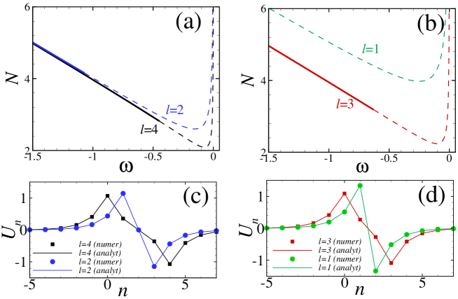
Figure 6: (Color online) Panels (a) and (b) display $N(\omega)$ curves for families of the antisymmetric solutions of on-site and inter-site types, respectively (i.e., even or odd distance $l$ between the nonlinear sites). The solid and dashed portions of the curves refer, as usual, to stable and unstable solutions. Panels (c) and (d) display typical profiles of the antisymmetric on-site and inter-site modes, as obtained in the numerical and analytical forms at $\omega=-0.5$.

To check the linear-stability predictions for the antisymmetric modes, we took initial profiles of the antisymmetric solutions from Fig. 6(c),(d) at $\omega=-0.5$, when the on-site/inter-site modes with $l=1,2,3$ are unstable, while the one with $l=4$ is stable, and simulated Eq. (1) with small initial perturbations ($\sim 1\%$). The results are presented in Fig. 7. The unstable solutions spontaneously transform into single-peak modes localized on one of the nonlinear sites, which demonstrates decaying oscillations of the amplitude. On the other hand, the linearly stable antisymmetric mode, with $l=4$, is indeed robust in the direct simulations.

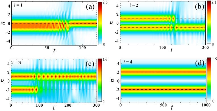
Figure 7: (Color online) The evolution of unstable (a), (b), (c) and stable (d) antisymmetric modes. Initial profiles are taken from Fig. 6(c),(d) with $\omega=-0.5$, for $l=1,2,3,4$.

IV.4 Effects of the finite extension of the nonlinear region

In the model with two finite nonlinearity domains, defined as per Eq. (3), results were obtained in the numerical form. They are displayed for the families of symmetric and asymmetric modes in Fig. 8, and for the antisymmetric ones in Fig. 9. In particular, Fig. 8 demonstrates that the increase of the width of the nonlinearity domain transforms the subcritical bifurcation into a supercritical one, thus completely stabilizing the asymmetric modes and making the value of $N$ at the SBB point lower. It is also worthy to note that, as seen in Fig. 9, the broader nonlinearity gives rise to an additional stability window close to the existence threshold (minimum value of $N$).

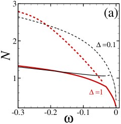
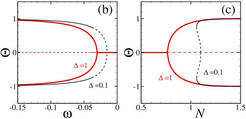
Figure 8: (Color online) (a) Curves $N(\omega)$ of the symmetric and asymmetric solution families for $l=4$ with $\Delta=0.1$ in Eq. (3) (black thin lines, which are actually tantamount to their counterparts with the $\delta$-like nonlinearity), and with $\Delta=1$ (red thick lines), which correspond to a relatively broad Gaussian. In (b) and (c), the corresponding asymmetry ratio $\Theta$ is shown versus $\omega$ and $N$.

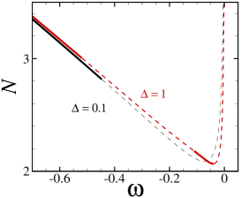
Figure 9: (Color online) The $N(\omega)$ curves of antisymmetric solution families for $l=4$ with $\Delta=0.1$ (black curves) and $\Delta=1$ (red curves), cf. Fig. 8.

V The ring model

If the infinite linear chain is replaced by a circle (ring) with the nonlinear sites placed at diametrically opposite points, Eq. (2) is replaced by the following one:

$$\omega U_{n}+\frac{1}{2}\left(U_{n+1}+U_{n-1}-2U_{n}\right)+\left(\delta_{n,n_{-}}+\delta_{n,n_{+}}\right)U_{n}^{3}=0,$$ (24)

where $n=n_{\pm}$ may be defined as the top and bottom points of a vertical diameter cutting the circle. In fact, it is more convenient to replace Eq. (24) by a system of two identical equations for two semi-circles, left and right ones. In each equation, $n$ takes values $n_{-}<n<n_{+}$ ($n_{-}<0$ and $n_{+}>0$ are assumed). In BEC, the circular chain can be realized as a combination of a toroidal trap and periodic potential created in it torus , and in optics it corresponds to an array of waveguides created in a hollow cylindrical shell, or written in the form of the ring in a bulk sample Jena .

In principle, one may expect two types of the symmetry breaking in this setting: between the top and bottom, which is a counterpart of what was considered above in the framework of the rectilinear chain, or between the left and right semi-circles.

The linear solutions for the left ($l$) and right ($r$) semi-circles can be looked for as

$$\left(U_{n}\right)_{l,r}=A_{l,r}\cosh\left(\kappa\left(n-n_{l,r}\right)\right),$$ (25)

with $\kappa$ related to $\omega$ by Eq. (5), and some constants $A_{l,r}$ and $n_{l,r}$ ($n_{l}$ and $n_{r}$ are not necessarily integer numbers). Then, the continuity conditions should be imposed at points $n=n_{\pm}$, where the two semi-circles are linked into the entire circle:

$$A_{l}\cosh\left(n_{\pm}-n_{l}\right)=A_{r}\cosh\left(n_{\pm}-n_{r}\right).$$ (26)

After simple manipulations, one may eliminate the amplitudes from two equations (26), which leads to the following consistency condition: $\cosh\left(\kappa\left(n_{+}-n_{-}-n_{l}+n_{r}\right)\right)=\cosh\left(\kappa\left(n_{+}-n_{-}+n_{l}-n_{r}\right)\right).$ It is obvious that the consistency condition can be met in the case of $n_{+}=n_{-}$, which is trivial (zero length of the ring), or

$$n_{l}=n_{r}\equiv n_{0}.$$ (27)

Further, it then follows from Eqs. (26) that a consequence of Eq. (27) is $A_{l}=A_{r}\equiv A$, hence the symmetry breaking between the left and right circles is impossible.

However, the top-bottom symmetry breaking is possible. Substituting ansatz (25) with the left-right symmetry into Eq. (24) at points $n=n_{\pm}$, the result of a straightforward analysis is a system of two equations, corresponding to $+$ and $-$:

$$\tanh\left(\kappa\left(n_{\pm}-n_{0}\right)\right)\left[1-\tanh^{2}\left(\kappa\left(n_{\pm}-n_{0}\right)\right)\right]=\pm A^{2}/\sinh\kappa\text{,}$$ (28)

where $n_{0}$ is defined as per Eq. (27). In equations (28), $A^{2}$ and $n_{0}$ are considered as two unknowns, for given $\kappa$ and $n_{\pm}$. As follows from Eqs. (28), the symmetric solution, with $n_{0}=\left(1/2\right)\left(n_{+}+n_{-}\right)$, has amplitude

$$A_{\mathrm{symm}}^{2}=\left(\sinh\kappa\right)\tanh\left(\left(\kappa/2\right)\left(n_{+}-n_{-}\right)\right)\left[1-\tanh^{2}\left(\left(\kappa/2\right)\left(n_{\pm}-n_{0}\right)\right)\right].$$ (29)

An obvious corollary of Eqs. (28) is relation

$$\tanh\left(\kappa\left(n_{+}-n_{0}\right)\right)\left[1-\tanh^{2}\left(\kappa\left(n_{+}-n_{0}\right)\right)\right]-\tanh\left(\kappa\left(n_{0}-n_{-}\right)\right)\left[1-\tanh^{2}\left(\kappa\left(n_{0}-n_{-}\right)\right)\right]=0.$$ (30)

The SBB point can be found by setting $n_{0}=\left(1/2\right)\left(n_{+}-n_{-}\right)+\delta n_{0}$, with infinitesimal $\delta n_{0}$, and demanding that the coefficient in front of $\delta n_{0}$ in the respective expansion of the left-hand side of Eq. (30) vanishes. The result is that this happens at point $\cosh\left(\left(\kappa/2\right)\left(n_{+}-n_{-}\right)\right)=\sqrt{3/2},$ which is equivalent to

$$\left[\kappa\left(n_{+}-n_{-}\right)\right]_{\mathrm{cr}}=\ln\left(2+\sqrt{3}\right).$$ (31)

At this point, the amplitude is

$$A_{\mathrm{cr}}^{2}=\left(2/3^{3/2}\right)\sinh\kappa.$$ (32)

The asymmetric state exists, for given $\kappa$, i.e., given $\omega$, for the length of the semi-circle, $n_{+}-n_{-}$, which is larger than the one corresponding to Eq. (31). Alternatively, at given $n_{+}-n_{-}$, the asymmetric state exists for $\kappa$ exceeding the value defined by Eq. (31).

In Fig. 10 we summarize the results related to the ring configuration. In panel (a), families of the symmetric and asymmetric solutions are displayed for three different lengths of the ring. We have checked the linear stability of the corresponding solutions through the numerical computation of the eigenvalues for small perturbations. The respective stable and unstable regions of the existence curves are shown by the solid and dashed lines, respectively. As in the case of the linear chain, at critical frequency $\omega_{\mathrm{cr}}$ calculated from Eq. (31), the branches of the asymmetric solutions bifurcate from the branch of symmetric solutions. The amplitude of the symmetric solutions at the bifurcation point is displayed in Fig. 10(b) for different lengths of the ring.

Also for different lengths of the ring, we have analyzed the type of the corresponding SBB, calculating the asymmetry parameter $\Theta$ as per Eq. (20). The dependences of $\Theta$ on frequency $\omega$ and norm $N$ are shown in Figs. 10(c) and (d). As one can see, the length of the ring plays a crucial role in the determination of the bifurcation type. In the small ring (e.g., of length 6), the bifurcation is supercritical, while the increase the length to $\geq 8$ changes it into a subcritical one.

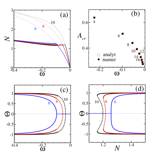
Figure 10: (Color online) (a): The family of symmetric (thin) and asymmetric (thick) solutions for three different lengths of the ring (6, 8, and 10). The solid and dashed lines correspond to the stable and unstable solutions, respectively. (b): The amplitude of the symmetric solution at the bifurcation point, for different lengths of the ring (indicated by numbers at the points). (c), (d): The dependence of asymmetry $\Theta$ on the frequency (c) and norm $N$ (d), showing the change of the bifurcation type in the ring with the increase of the ring’s size.

In Figs. 11 and 12, the evolution of stable and unstable asymmetric and symmetric solutions is shown. The direct simulations corroborate the linear-stability analysis. As one can see, the solutions taken on stable parts of the existence curves are stable indeed. The unstable asymmetric solution [see Fig. 11(b)] starts to oscillate between two asymmetric configurations, while the unstable symmetric solution in Fig. 12(b) rapidly transforms into an oscillating single-peak mode. It is relevant to stress that, similar to the situation in the straight chain (cf. Fig. 5), the instability of symmetric modes transforms them into asymmetric ones, while the instability of asymmetric modes leads to the emergence of the effective dynamical symmetry.

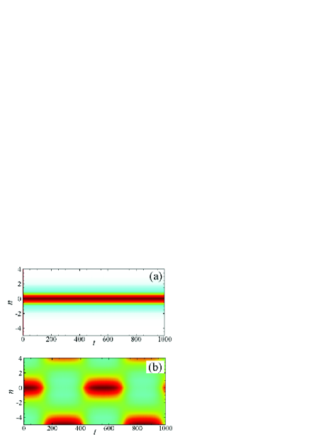
Figure 11: (Color online) The evolution of stable (a) and unstable (b) asymmetric solutions with initial profiles taken at $\omega=-0.5$ and $\omega=-0.05$, respectively. The length of the ring is 10 sites. Initial profiles were taken with small perturbations.

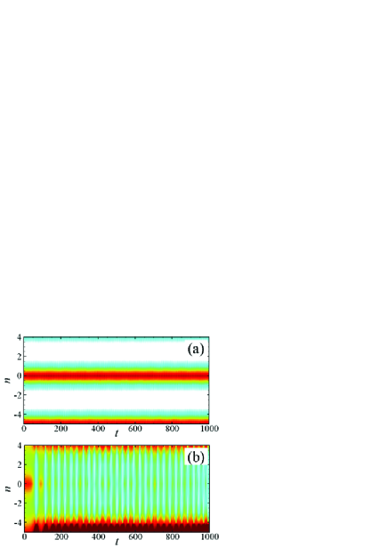
Figure 12: (Color online) The evolution of stable (a) and unstable (b) symmetric solutions with initial profiles taken at $\omega=-0.05$ and $\omega=-0.03$, respectively. The length of the ring is 10 sites. Initial profiles were taken with small perturbations.

Finally, it is relevant to note that, in the case of the circle of a finite length, it is also possible to consider values $\omega>0$, i.e., imaginary wavenumbers, $\kappa=i|\kappa|$, see Eq. (5). This means that the exponentially decaying discrete waves are replaced by oscillatory ones. After a simple analysis, the respective version of Eq. (28) can be derived in the following form:

$$\tan\left(|\kappa|\left(n_{\pm}-n_{0}\right)\right)\left[1+\tan^{2}\left(|\kappa|\left(n_{\pm}-n_{0}\right)\right)\right]=\mp A^{2}/\left[2\sin\left(|\kappa|\right)\right]\text{.}$$ (33)

A straightforward analysis of Eq. (33) demonstrates that, on the contrary to Eq. (28), it does not give rise to the symmetry breaking (the crucial difference is the opposite sign in front of $\tan^{2}$ in the square brackets).

VI Conclusion

The objective of this work is to elaborate the simplest setting for the study of the spontaneous symmetry breaking in dynamical chains. For this purpose, we have introduced two one-dimensional discrete systems, in the form of the straight and ring-shaped linear chains, with two symmetrically inserted nonlinear sites. This pair of sites introduces the symmetry that may be spontaneously broken. The chains, both rectilinear and circular ones, can be realized in BEC (with the help of optical lattices) and in optics, in the form of waveguiding arrays. A full set of analytical solutions for symmetric, asymmetric, and antisymmetric localized states has been obtained in the explicit form, for both geometries. The stability of the stationary modes was investigated through the numerical computation of the eigenvalues for small perturbations. The SBB (symmetry-breaking bifurcation), which is responsible for the asymmetric modes emerging from the symmetric ones, is of the subcritical type in the straight lattice, and in the circular one of a sufficiently large size. The bifurcation becomes supercritical if the system is made effectively nonlocal, i.e., in the ring of a smaller size, or if the nonlinearity is spread over relatively broad areas around the two central sites in the straight chain. The antisymmetric modes are not subject to bifurcations, although they too may be both stable and unstable. The development of the instability (when it occurs) was tested with the help of direct simulations. It was found that the unstable stationary asymmetric states, which are a part of the subcritical bifurcation, spontaneously transform into breathers oscillating between the two nonlinear sites, that may be considered as the restoration of an effective dynamical symmetry.

References

- (1) D. Landau and E. M. Lifshitz, Quantum Mechanics (Moscow: Nauka Publishers, 1974).
- (2) S. Giorgini, L. P. Pitaevskii, and S. Stringari, Rev. Mod. Phys. 80, 1215 (2008); H. T. C. Stoof, K. B. Gubbels, and D. B. M. Dickrsheid, Ultracold Quantum Fields (Springer: Dordrecht, 2009).
- (3) Y. S. Kivshar and G. P. Agrawal, Optical Solitons: From Fibers to Photonic Crystals (Academic Press: San Diego).
- (4) E. A. Ostrovskaya, Y. S. Kivshar, M. Lisak, B. Hall, F. Cattani, and D. Anderson, Phys. Rev. A 61, 031601(2000); R. D’Agosta, B. A. Malomed, C. Presilla, Phys. Lett. A 275, 424 (2000); R. K. Jackson and M. I. Weinstein, J. Stat. Phys. 116, 881 (2004); D. Ananikian and T. Bergeman, Phys. Rev. A 73, 013604 (2006); E. W. Kirr, P. G. Kevrekidis, E. Shlizerman, and M. I. Weinstein, SIAM J. Math. Anal. 40, 566 (2008).
- (5) G. J. Milburn, J. Corney, E. M. Wright, and D. F. Walls, Phys. Rev. A 55, 4318 (1997); A. Smerzi, S. Fantoni, S. Giovanazzi, and S. R. Shenoy, Phys. Rev. Lett. 79, 4950 (1997); S. Raghavan, A. Smerzi, S. Fantoni, and S. R. Shenoy, Phys. Rev. A 59, 620 (1999); K. W. Mahmud, H. Perry, and W. P. Reinhardt, Phys. Rev. A 71, 023615 (2005); E. Infeld, P. Ziń, J. Gocalek, and M. Trippenbach, Phys. Rev. E 74, 026610 (2006); G. Theocharis, P. G. Kevrekidis, D. J. Frantzeskakis, and P. Schmelcher, Phys. Rev. E 74, 056608 (2006); G. L. Alfimov and D. A. Zezyulin, Nonlinearity 20, 2075 (2007); C. Wang, P. G. Kevrekidis, N. Whitaker, and B. A. Malomed, Physica D 237, 2922 (2008).
- (6) M. Albiez, R. Gati, J. Fölling, S. Hunsmann, M. Cristiani, and M. K. Oberthaler, Phys. Rev. Lett. 95, 010402 (2005); R. Gati, M. Albiez, J. Fölling, B. Hemmerling, and M. K. Oberthaler, Appl. Phys. B 82, 207 (2006).
- (7) P. G. Kevrekidis, Z. Chen, B. A. Malomed, D. J. Frantzeskakis, and M. I. Weinstein, Phys. Lett. A 340, 275 (2005).
- (8) J. C. Eilbeck, P. S. Lomdahl, and A. C. Scott, Physica D 16, 318 (1985).
- (9) A. W. Snyder, D. J. Mitchell, L. Poladian, D. R. Rowland, and Y. Chen, J. Opt. Soc. Am. B 8, 2101 (1991).
- (10) C. Paré and M. Fłorjańczyk, Phys. Rev. A 41, 6287 (1990); A. I. Maimistov, Kvant. Elektron. 18, 758 [Sov. J. Quantum Electron. 21, 687 (1991)]; N. Akhmediev and A. Ankiewicz, Phys. Rev. Lett. 70, 2395 (1993); P. L. Chu, B. A. Malomed, and G. D. Peng, J. Opt. Soc. A B 10, 1379 (1993); B. A. Malomed, in: Progr. Optics 43, 71 (E. Wolf, editor: North Holland, Amsterdam, 2002).
- (11) W. C. K. Mak, B. A. Malomed, and P. L. Chu, J. Opt. Soc. Am. B 15, 1685 (1998).
- (12) A. Gubeskys and B. A. Malomed, Phys. Rev. A 75, 063602 (2007).
- (13) M. Matuszewski, B. A. Malomed, and M. Trippenbach, Phys. Rev. A 75, 063621 (2007).
- (14) M. Trippenbach, E. Infeld, J. Gocalek, M. Matuszewski, M. Oberthaler, and B. A. Malomed, Phys. Rev. A 78, 013603 (2008).
- (15) L. Salasnich, B. A. Malomed, and F. Toigo, Phys. Rev. A 81, 045603 (2010).
- (16) G. Iooss and D. D. Joseph, Elementary Stability Bifurcation Theory (Springer-Verlag: New York, 1980).
- (17) W. A. Harrison, Pseudopotentials in the Theory of Metals (Benjamin: New York, 1966).
- (18) L. C. Qian, M. L. Wall, S. Zhang, Z. Zhou, and H. Pu, Phys. Rev. A 77, 013611 (2008).
- (19) Y. V. Kartashov, B. A. Malomed, and L. Torner, Solitons in nonlinear lattices, Rev. Mod. Phys., in press.
- (20) T. Mayteevarunyoo, B. A. Malomed, and G. Dong, Phys. Rev. A 78, 053601 (2008).
- (21) N. Dror and B. A. Malomed, Solitons supported by localized nonlinearities in periodic media, Phys. Rev. A 83, 033828 (2011).
- (22) N. V. Hung, P. Ziń, M. Trippenbach, and B. A. Malomed, Phys. Rev. E 82, 046602 (2010).
- (23) B. A. Malomed and M. Ya. Azbel, Phys. Rev. B 47, 10402 (1993).
- (24) G. Herring, P. G. Kevrekidis, B. A. Malomed, R. Carretero-González, and D. J. Frantzeskakis, Phys. Rev. E 76, 066606 (2007).
- (25) Lj. Hadžievski, G. Gligorić, A. Maluckov, and B. A. Malomed, Phys. Rev. A 82, 033806 (2010).
- (26) M. Vakhitov and A. Kolokolov, Radiophys. Quantum. Electron. 16, 783 (1973); L. Bergé, Phys. Rep. 303, 259 (1998).
- (27) P. O. Fedichev, Y. Kagan, G. V. Shlyapnikov, and J. T. M. Walraven, Phys. Rev. Lett. 77, 2913 (1996); M. Theis, G. Thalhammer, K. Winkler, M. Hellwig, G. Ruff, R. Grimm, and J. H. Denschlag, ibid. 93, 123001 (2004).
- (28) J. Hukriede, D. Runde, and D. Kip, J. Phys. D: Appl. Phys. 36, R1 (2003).
- (29) B. A. Malomed and M. I. Weinstein, Soliton dynamics in the discrete nonlinear Schrödinger equation, Phys. Lett. A 220, 91-96 (1996); D. J. Kaup, Mathematics and Computers in Simulations 69, 322 (2005); R. Carretero-González, J. D. Talley, C. Chong, and B. A. Malomed, Physica D 216, 77 (2006).
- (30) R. Y. Chiao, E. Garmire, and C. H. Townes, Phys. Rev. Lett. 13, 479 (1964); L. Bergé, Phys. Rep. 303, 259 (1998).
- (31) S. Gupta, K. W. Murch, K. L. Moore, T. P. Purdy, and D. M. Stamper-Kurn, Phys. Rev. Lett. 95, 143201 (2005); I. Lesanovsky and W. von Klitzing, ibid. 99, 083001 (2007); B. E. Sherlock, M. Gildemeister, E. Owen, E. Nugent, and C. J. Foot, arXiv:1102.2895v2.
- (32) A. Szameit, J. Burghoff, T. Pertsch, S. Nolte, A. Tünnermann, and F. Lederer, Opt. Exp. 14, 6055 (2006); A. Szameit and S. Nolte, J. Phys. B: At. Mol. Opt. Phys. 43, 163001 (2010).