Cool DZ white dwarfs in the SDSS

Abstract

Aims. We report the identification of 26 cool DZ white dwarfs that lie across and below the main sequence in the Sloan Digital Sky Survey (SDSS) $(u-g)$ vs. $(g-r)$ two-color diagram; 21 of these stars are new discoveries.

Methods. The sample was identified by visual inspection of all spectra of objects that fall below the main sequence in the two-color diagram, as well as by an automated search for characteristic spectral features over a large area in color space that included the main sequence. The spectra and photometry provided by the SDSS project are interpreted with model atmospheres, including all relevant metals. Effective temperatures and element abundances are determined, while the surface gravity has to be assumed and was fixed at the canonical value of $\log\leavevmode\nobreak\ g$ = 8.

Results. These stars represent the extension of the well-known DZ sequence towards cooler temperatures and fill the gap around $T_{\mathrm{eff}}$ = 6500 K present in a previous study. The metal abundances are similar to those in the hotter DZ, but the lowest abundances are missing, probably because of our selection procedures. The interpretation is complicated in terms of the accretion/diffusion scenario, because we do not know if accretion is still occurring or has ended long ago. Independent of that uncertainty, the masses of the metals currently present in the convection zones – and thus an absolute lower limit of the total accreted masses – of these stars are similar to the largest asteroids in our solar system.

1 Introduction

Cool white dwarfs with traces of metals other than carbon are designated with the letter “Z” in the current classification system. If Balmer lines are visible, they are called DAZ or DZA, depending on whether hydrogen lines or some metal lines are the strongest. Helium-dominated DBs with metals are DBZ, and finally, at lower temperature where no hydrogen or helium lines remain visible, there are the DZs. Helium-rich DBZs and DZs have been known for a long time; in fact, one of the first three classical white dwarfs, van Maanen 2, belongs to this class (Kuiper 1941). DAZs were discovered much later (Koester et al. 1997; Holberg et al. 1997), but this is purely observational bias, since the metal line strengths are much weaker in hydrogen atmospheres with lower transparency.

The almost mono-elemental composition of the outer layers is caused by gravitational settling, with time scales much shorter than the white dwarf evolutionary time scales. The metals can therefore not be primordial. For decades the standard explanation has been accretion from interstellar matter (ISM), with subsequent diffusion downward out of the atmosphere. This scenario has been discussed in detail and compared with observations in a series of three fundamental papers by Dupuis et al. (1992, 1993a, 1993b). A special case is the DQ spectral class, with pollution by the element carbon. The carbon can be dredged-up from below the outer helium layer by a deepening convection zone and does not necessarily need an exterior source (Koester et al. 1982; Pelletier et al. 1986).

The ISM accretion hypothesis for the DZ has a number of problems, the most disconcerting ones being the lack of dense interstellar clouds in the solar neighborhood, and in many cases a large deficit of hydrogen in the accreted matter. These arguments have been summarized by Farihi et al. (2010a), who in the same paper argue for the accretion of circumstellar dust as the source of the accreted matter. This dust is thought to originate from the the tidal disruption of some rocky material, left over from a former planetary system (Debes & Sigurdsson 2002; Jura 2003). This idea has gained more and more acceptance in the last decade, mainly through the discovery of infrared excesses due to circumstellar dust in a significant fraction of DAZs and DBZs (Jura 2006; von Hippel et al. 2007; Farihi et al. 2009, 2010b, 2010a). In particular the gaseous disks with Ca ii emission lines (Gänsicke et al. 2006, 2007, 2008) are the strongest confirmation for the disk geometry and its location inside the Roche lobe of the white dwarfs, a key prediction of the tidal disruption hypothesis.

A sample of 147 cool He-rich metal polluted white dwarfs (spectral class DZ) identified by SDSS has been analyzed by Dufour et al. (2007). Of these, only two have $T_{\mathrm{eff}}$ below 6600 K (at 6090 and 4660 K). Given that already about half a dozen cool DZ known within 20 pc of the Sun are brighter than this SDSS sample (including van Maanen 2 at only 4.3 pc, Sion et al. 2009) this suggests that a large number of cooler DZ remain to be found.

2 Color selection

We have been investigating the spectroscopic data base for white dwarfs with unusual properties (Gänsicke et al. 2010), and identified SDSS0916+2540 (which we adopt as notation for SDSS objects throughout this paper) as a cool, very metal-rich DZ white dwarf. In the $(u-g)$ vs. $(g-r)$ color-color diagram, this star lies below the main sequence, a region that has hitherto not been systematically explored for its stellar content. SDSS intensively targeted this region as part of its quasar program (Richards et al. 2002). Inspecting all spectroscopic objects within SDSS Data Release 7 (Abazajian et al. 2009) that have colors within the dashed region shown in Fig. 1 confirms that the vast majority are $z\sim 3$ quasars, however, we also identified 16 of these objects as cool DZ white dwarfs characterized by a strong complex of MgI absorption lines near 5170 Å (one of these turned out to be a carbon-rich DQ, see below). This finding, coupled with the fact that all except one of the SDSS DZ stars analyzed by Dufour et al. (2007) are located above the main sequence in $(u-g)$ vs. $(g-r)$ (Fig. 1) strongly suggested that part of the DZ population will fall right into the color space occupied by the main sequence. In the view of the large number of DR7 spectra of $\sim$K-A type stars we developed a search routine in the region bounded by the solid lines in Fig. 1, which checks for the characteristic spectral features, foremost the Mg i lines near 5170 Å. Secondary criteria were the presence of the Na D lines and the absence of H$\alpha$. A heavy contamination are still K stars with molecular bands of MgH, but since the slope of the spectrum is quite different, they can be identified by visual inspection. This procedure led to the discovery of nine additional DZ white dwarfs, two of which were already in the Dufour sample. Two additional objects, SDSS0143+0113 and SDSS2340+0817, were identified independently by Dufour in a search for DZs. The complete list of cool DZ (plus one DQ) white dwarfs identified and their $ugriz$ photometry is given in Table 1.

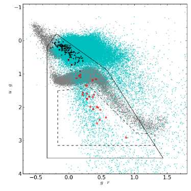
Figure 1: SDSS Two-color diagram for objects with spectra identified as normal stars (grey S-shaped region in the middle of the figure), QSO (cyan dots), DZ white dwarfs analyzed by Dufour et al. (2007) (solid black dots) and cool “extreme” DZ discovered by our search (red open circles).

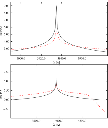
Figure 2: Quasi-static line profile for the Ca ii K resonance line (dashed, red), compared with the impact approximation (continuous, black). Parameters are 6000 K for the temperature and a neutral He perturber density of $10^{19}$cm^-3. The central region is enlarged in the top panel. The quasi-static calculation is only useful for the wing; approximately within the central region between the crossing points of the two profiles the impact calculation is the superior approximation.

Table 1: DZ white dwarfs in the sample

SDSS	plate-MJD-fib	$u$	$g$	$r$	$i$	$z$
014300.52+011356.8	53265-1907-405	20.410 (0.060)	19.380 (0.010)	19.200 (0.010)	19.260 (0.020)	19.390 (0.060)
015748.14+003315.0	52199-0700-627	21.261 (0.096)	19.566 (0.020)	19.120 (0.017)	19.237 (0.027)	19.353 (0.053)
020534.13+215559.7	53349-2066-223	21.076 (0.097)	19.916 (0.019)	19.502 (0.017)	19.446 (0.021)	19.430 (0.057)
091621.36+254028.4	53415-2087-166	21.258 (0.102)	18.346 (0.013)	17.473 (0.016)	17.384 (0.016)	17.528 (0.019)
092523.10+313019.0	53379-1938-608	21.039 (0.105)	18.983 (0.019)	18.611 (0.015)	18.632 (0.015)	18.748 (0.045)
093719.14+522802.2	53764-2404-197	20.780 (0.067)	19.439 (0.029)	19.178 (0.019)	19.301 (0.022)	19.370 (0.055)
095645.14+591240.6	51915-0453-621	18.971 (0.024)	18.394 (0.018)	18.399 (0.021)	18.554 (0.020)	18.743 (0.040)
103809.19$-$003622.4	51913-0274-265	17.710 (0.020)	16.984 (0.021)	16.940 (0.014)	17.087 (0.013)	17.308 (0.017)
104046.48+240759.5	53770-2352-004	21.717 (0.147)	19.337 (0.025)	18.866 (0.018)	18.870 (0.023)	19.102 (0.063)
104319.84+351641.6	53431-2025-328	20.642 (0.077)	18.959 (0.020)	18.647 (0.020)	18.611 (0.017)	18.665 (0.038)
110304.15+414434.9	53046-1437-410	21.718 (0.186)	19.731 (0.027)	19.403 (0.020)	19.385 (0.021)	19.425 (0.057)
114441.92+121829.2	53138-1608-515	20.723 (0.085)	18.412 (0.018)	17.846 (0.019)	17.755 (0.019)	17.758 (0.022)
115224.51+160546.7	53415-1762-522	21.728 (0.131)	20.169 (0.025)	19.954 (0.021)	20.012 (0.031)	20.103 (0.092)
123415.21+520808.1	52379-0885-269	19.545 (0.042)	18.415 (0.024)	18.299 (0.018)	18.424 (0.015)	18.681 (0.032)
133059.26+302953.2	53467-2110-148	18.300 (0.022)	16.310 (0.016)	15.885 (0.012)	15.898 (0.025)	16.095 (0.024)
133624.26+354751.2	53858-2101-254	19.481 (0.027)	17.854 (0.015)	17.643 (0.013)	17.717 (0.027)	17.827 (0.018)
135632.63+241606.0	53792-2119-216	20.351 (0.057)	18.998 (0.026)	18.721 (0.016)	18.741 (0.019)	18.814 (0.044)
140410.72+362056.8	54590-2931-302	20.010 (0.041)	18.818 (0.029)	18.454 (0.018)	18.520 (0.021)	18.692 (0.033)
140557.10+154940.5	54272-2744-586	20.000 (0.043)	18.940 (0.020)	18.785 (0.019)	18.901 (0.018)	19.104 (0.042)
142120.11+184351.6	54533-2773-088	22.096 (0.168)	20.355 (0.031)	20.077 (0.024)	20.194 (0.037)	20.329 (0.110)
143007.15$-$015129.5	52409-0919-358	21.485 (0.141)	19.475 (0.021)	19.031 (0.021)	18.993 (0.019)	19.090 (0.061)
152449.58+404938.1	54626-2936-537	21.760 (0.120)	20.135 (0.028)	19.752 (0.021)	19.765 (0.027)	19.808 (0.078)
153505.75+124744.2	54240-2754-570	18.054 (0.024)	15.977 (0.020)	15.497 (0.018)	15.452 (0.022)	15.504 (0.017)
154625.33+300946.2	53142-1390-362	21.398 (0.085)	19.807 (0.020)	19.528 (0.018)	19.647 (0.023)	19.794 (0.063)
155429.01+173545.9	53875-2170-154	18.698 (0.024)	17.599 (0.015)	17.420 (0.011)	17.468 (0.011)	17.650 (0.023)
161603.00+330301.2	53239-1684-340	21.006 (0.095)	19.252 (0.018)	18.973 (0.020)	19.069 (0.019)	19.154 (0.045)
234048.74+081753.3	54326-2628-108	22.733 (0.273)	20.248 (0.020)	19.819 (0.020)	19.871 (0.027)	19.953 (0.075)

3 Input physics and models

3.1 Line identification and broadening

All spectral features found in the spectra of the new cool DZ white dwarfs can be identified with lines from Ca, Mg, Na, Fe, Ti, and Cr, broadened predominantly through van der Waals broadening by neutral helium. The broadest lines show strongly asymmetric profiles, which were in the case of Mg i 5169/5174/5185 originally identified as due to quasi-static broadening by Wehrse & Liebert (1980) in their study of SDSS1330+3029 (= G165-7). The same conclusion was reached by Kawka et al. (2004) for SDSS1535+1247; both of these stars are in our present sample. The width of these lines, as well as that of the Ca ii resonance lines is far beyond the range of validity of the impact approximation, which is in these cases approximately 8-10 Å from the line centers (see p. 312 in Unsöld 1968). We have used the simple and elegant method of Walkup et al. (1984), who present numerical calculations for the transition range between impact and quasi-static regime, which can in both limits be easily extended with the asymptotic formulae. These profiles are reasonable approximations for the MgI triplet.

For the much wider Ca ii resonance lines this approximation fails. The reason is very likely that for such strong interactions needed to produce a 600 Å wide wing the approximation with a simple van der Waals $r^{-6}$ law is not valid. We have used the quasi-static limit of the semiclassical quasi-molecular broadening theory as described in Allard & Kielkopf (1982). This formulation (e.g. their eq. 59 in the cited paper) easily allows the incorporation of a Boltzmann factor to account for the variation of the perturbation probability with distance of the perturber in thermal equilibrium. It would also allow us to take a variation in the dipole moments into account, which, however, are apparently not available in the published literature.

Adiabatic potential energy curves for the ground state of the Ca⁺He quasi-molecule and the two exited states correlated with the resonance term of the Ca ii ion – (4p)${}^{2}\Sigma$ and (4p)${}^{2}\Pi$ – were calculated by Czuchaj et al. (1996) and numerical data were presented in a table. Approximate calculations for the spin-orbit interaction show a mixing of the two upper levels of the doublet and a complicated structure of the energy curves (their Fig. 4). Since no numerical data are given for these calculations, we use the potential curves without this interaction.

These profiles (Fig. 2) were used in the calculation of models and provide a fairly good fit for the red wing; the blue wing is mostly outside the SDSS wavelength range. Nevertheless, the current analysis is only a first attempt with a number of shortcomings:

• A more accurate description of the line profile needs to take into account the spin-orbit interaction and the variation of the dipole moments.

• The potential curves are calculated only to the closest distance of $\approx$ 1.6 Å, since the authors were interested in possible minima and bound states of the molecule. The distant wings of the profile depend somewhat on how the potential is extrapolated to shorter distances.

• Since the Ca ii ion has a net charge, the interaction with the He atom has a polarization term with a $r^{-4}$ dependence on separation, which dominates at large distances. This is different from the case of a neutral radiator, where the potential is the van der Waals $r^{-6}$ type. However, since the polarization term is the same for upper and lower state, it cancels out in the difference, which is the important quantity for line broadening. In principle the $r^{-6}$ term should remain, but might be distorted by numerical noise. To avoid that, we have replaced the potential difference at large distances by an accurate van der Waals term, which allows us to recover a reasonable profile also near the line center.

• The quasi-static calculation is valid only in the wings. Within approximately 20 Å of the line center the impact approximation would be a better description. A complete calculation of the unified profile similar to the calculations for the Na and K resonance lines by Allard et al. (2003) would be desirable. Nevertheless, since the Ca ii resonance lines are strongly saturated in the line centers, the unsatisfactory description of the line core does not affect our results.

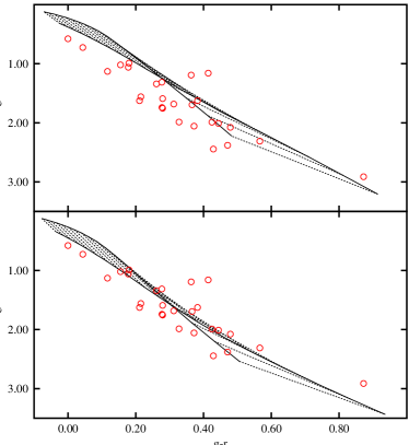
Figure 3: Observed and model colors in the $u-g$ vs. $g-r$ two-color diagram. Top panel: the continuous lines are model values for a temperature sequence from 5400 K (lower right) to 9000 K (upper left) with steps of 200 K. The dotted lines connect the same $T_{\mathrm{eff}}$ for 2 different abundances; the upper line in the right half of the figure corresponds to abundances of SDSS0916+2540, the other line to SDSS1103+4144. The (red) circles are the observed data. Bottom panel: the same models, but with the neutral broadening constant for the Mg ii resonance lines increased by a factor of 10 to simulate a stronger blanketing effect in the near ultraviolet.

Table 2: Lines identified in SDSS0916+2540

Ion	Wavelengths
	[Å]
Ca i	4227.918, 5590.301, 5596.015, 5600.034
	6104.413, 6123.912, 6163.878, 6440.855
	6464.353, 6495.575, 7150.121, 7204.185
Ca ii	3934.777, 3964.592, 8544.438, 8664.520
Mg i	5168.761, 5174.125, 5185.047
Fe i	4384.775, 4405.987, 5271.004, 5271.823
	5329.521, 5372.982, 5398.627, 5407.277
	5431.205, 5448.430
Ti i	4534.512, 4536.839, 4537.190, 4537.313
	4983.121, 4992.457, 5000.897, 5008,607
	5015.586, 5015.675, 5041.362, 5066.065
Cr i	5207.487, 5209.875
Na i	5891.583, 5897.558

3.2 Atmospheric parameters from photometry

By iteration through trial and error we have determined $T_{\mathrm{eff}}$ and abundances and calculated a model, which gives a fairly good fit to the spectrum and photometry of the most feature-rich object, SDSS0916+2540. The parameters for this object are $T_{\mathrm{eff}}$ = 5500 K, $\log$[Mg/He] = $-6.9$, $\log$[Ca/He] = $-7.6$, $\log$[Fe/He]= $-7.1$ (number abundance ratios). We then calculated a sequence of models with these abundances from $T_{\mathrm{eff}}$ = 5000 K to  7000 K in steps of 100 K, and continued up to 9000 K in steps of 200 K, always assuming a surface gravity $\log g=8.0$. Similarly a second sequence was calculated with abundances appropriate for SDSS1103+4144 ($T_{\mathrm{eff}}$ = 5700 K, $\log$[Mg/He] = $-7.9$, $\log$[Ca/He] = $-9.7$, $\log$[Fe/He] = $-8.1$). The choice of this second object is somewhat arbitrary and was motivated by being most distant from the first sequence in $(u-g)$ vs. $(g-r)$ color space.

Convolving the spectral energy distribution with the $ugriz$ band-passes of the SDSS photometric system, we constructed the two-color $(u-g)$ vs. $(g-r)$ diagram shown in Fig. 3. Two conclusions can be drawn from this diagram

• The location of the theoretical models depends in a complicated way on metal abundance, which is caused by an interplay of direct absorption in the optical range, and an indirect effect of the blanketing by very strong absorption in the ultraviolet. It would be difficult to estimate abundances from the photometry.

• The observed objects form a temperature sequence, with some scatter caused by different relative abundances of Mg, Ca, and Fe. The general shape agrees with the theoretical grid, but the observations are shifted downward and to the left. This is a strong indication that we still underestimate the blanketing effect of the near ultraviolet spectral lines, although all expected strong lines of the detected metals, (most importantly Fe, Mg and Ca) are included in our models.

Table 3: Effective temperature and element abundances for the sample

SDSS	$T_{\mathrm{eff}}$(phot)	$T_{\mathrm{eff}}$	Mg	Ca	Fe	Na	other
	[K]	[K]
0143+0113	6600	6600	$-$7.4	$-$9.2	$-$7.7
0157+0033	6200	6300	$-$7.1	$-$8.1	$-$7.5
0205+2155	6000	6000					DQ 6000K C $-$7.0
0916+2540	5500	5500	$-$6.9	$-$7.6	$-$7.1	$-$9.3	Ti $-$9.0, Cr $-$8.9
0925+3130	5900	5900	$-$7.9	$-$9.3	$-$8.0	$-$9.3
0937+5228	7000	6900	$-$6.8	$-$8.3	$-$7.5
0956+5912	8600	8800	$-$5.5	$-$7.3	$-$6.5	$-$7.0	H $-$3.25
1038$-$0036	8300	8200	$-$6.6	$-$7.7	$-$7.2	$-$8.5	H $<$ $-$4.7
1040+2407	6100	6200	$-$7.1	$-$8.0	$-$7.2	$-$8.5
1043+3516	5800	5900	$-$8.1	$-$10.1	$-$7.8
1103+4144	5800	5700	$-$7.9	$-$9.7	$-$8.1	$-$9.0
1144+1218	5400	5300	$-$8.2	$-$9.9	$-$8.6
1152+1605	6900	6600	$-$7.3	$-$8.5	$-$7.4
1234+5208	7800	7800	$-$5.9	$-$7.5	$-$6.5	$-$8.2	Cr $-$8.2
1330+3029	6200	6440	$-$6.9	$-$8.1	$-$7.0	$-$8.4	H $\approx$-3
1336+3547	6600	6700	$-$7.1	$-$8.8	$-$7.6	$-$8.7	H $<$ $-$4.2
1356+2416	6100	6100	$-$7.7	$-$9.3
1404+3620	6600	5900	$-$7.9	$-$9.6	$-$8.6
1405+1549	7700	7700	$-$6.9	$-$8.1	$-$7.0
1421+1843	7200	6800	$-$6.9	$-$8.2	$-$7.1	$-$8.3
1430$-$0151	5700	6300	$-$6.4	$-$7.6	$-$6.8	$-$7.9	Ti $-$8.8, Cr $-$8.4
1524+4049	6000	5700	$-$7.9	$-$9.6	$-$7.9	$-$9.4
1535+1247	5600	6000	$-$7.3	$-$8.8	$-$7.6	$-$8.6	Ti $-$9.50, Cr $-$9.10
1546+3009	7200	6700	$-$7.2	$-$8.5	$-$7.0
1554+1734	7000	7000	$-$7.4	$-$8.7	$-$7.7	$-$8.5
1616+3303	6900	6700	$-$6.8	$-$8.5	$-$7.0
2340+0817	6300	6300	$-$7.5	$-$8.4	$-$7.5

Table 4: Comparison of observed SDSS photometry with theoretical colors for the final model

SDSS	$g$	$u-g$	$g-r$	$r-i$	$r-z$	SDSS	$g$	$u-g$	$g-r$	$r-i$	$i-z$
0143+0113	19.380	0.990	0.180	$-$0.060	$-$0.150	1330+3029	16.310	1.950	0.425	$-$0.012	$-$0.218
		0.886	0.207	$-$0.061	$-$0.123			1.493	0.362	$-$0.041	$-$0.151
		0.061	0.014	0.022	0.063			0.027	0.020	0.027	0.035
0157+0033	19.566	1.655	0.366	$-$0.037	$-$0.135	1336+3547	17.854	1.586	0.211	$-$0.074	$-$0.129
		1.263	0.442	$-$0.059	$-$0.164			0.865	0.225	$-$0.068	$-$0.136
		0.098	0.026	0.032	0.059			0.031	0.020	0.030	0.032
0916+2540	18.346	2.873	0.872	0.089	$-$0.164	1356+2416	18.998	1.313	0.277	$-$0.021	$-$0.092
		2.727	0.932	0.093	$-$0.193			0.949	0.329	$-$0.031	$-$0.103
		0.103	0.020	0.023	0.025			0.063	0.030	0.025	0.048
0925+3130	18.983	2.017	0.372	$-$0.021	$-$0.136	1404+3620	18.818	1.152	0.364	$-$0.065	$-$0.192
		1.471	0.383	$-$0.011	$-$0.095			1.103	0.358	$-$0.012	$-$0.088
		0.107	0.024	0.021	0.047			0.050	0.034	0.028	0.039
0937+5228	19.439	1.302	0.261	$-$0.123	$-$0.089	1405+1549	18.940	1.020	0.155	$-$0.115	$-$0.224
		0.754	0.233	$-$0.086	$-$0.161			0.561	0.111	$-$0.112	$-$0.189
		0.073	0.035	0.029	0.059			0.047	0.027	0.026	0.045
0956+5912	18.394	0.538	$-$0.005	$-$0.155	$-$0.209	1421+1843	20.355	1.701	0.278	$-$0.116	$-$0.156
		0.332	$-$0.003	$-$0.134	$-$0.219			1.011	0.270	$-$0.071	$-$0.163
		0.030	0.027	0.029	0.044			0.171	0.039	0.044	0.116
1038$-$0036	16.984	0.686	0.044	$-$0.146	$-$0.242	1430-0151	19.475	1.970	0.444	0.038	$-$0.117
		0.459	0.100	$-$0.147	$-$0.235			1.681	0.540	$-$0.021	$-$0.181
		0.029	0.025	0.019	0.021			0.143	0.030	0.028	0.064
1040+2407	19.337	2.341	0.471	$-$0.005	$-$0.251	1524+4049	20.135	1.586	0.382	$-$0.013	$-$0.063
		1.515	0.470	$-$0.036	$-$0.162			1.846	0.430	0.004	$-$0.081
		0.149	0.030	0.029	0.074			0.123	0.035	0.034	0.083
1043+3516	18.959	1.643	0.312	0.036	$-$0.074	1535+1247	15.977	2.037	0.479	0.045	$-$0.072
		1.769	0.335	$-$0.015	$-$0.085			1.573	0.425	$-$0.015	$-$0.113
		0.079	0.029	0.026	0.041			0.031	0.027	0.028	0.028
1103+4144	19.731	1.947	0.328	0.019	$-$0.060	1546+3009	19.807	1.551	0.279	$-$0.119	$-$0.167
		1.677	0.392	0.021	$-$0.078			1.153	0.275	$-$0.074	$-$0.147
		0.188	0.034	0.029	0.061			0.088	0.027	0.030	0.067
1144+1218	18.412	2.271	0.566	0.091	$-$0.024	1554+1734	17.599	1.060	0.178	$-$0.048	$-$0.202
		2.014	0.559	0.053	0.041			0.648	0.171	$-$0.073	$-$0.149
		0.087	0.026	0.027	0.029			0.028	0.018	0.016	0.026
1152+1605	20.169	1.519	0.215	$-$0.058	$-$0.111	1616+3303	19.252	1.714	0.279	$-$0.096	$-$0.104
		1.042	0.289	$-$0.068	$-$0.146			1.120	0.286	$-$0.075	$-$0.145
		0.133	0.032	0.037	0.097			0.096	0.026	0.027	0.049
1234+5208	18.415	1.090	0.117	$-$0.125	$-$0.278	2340+0817	20.248	2.445	0.429	$-$0.052	$-$0.102
		0.755	0.179	$-$0.122	$-$0.206			1.301	0.392	$-$0.055	$-$0.147
		0.049	0.030	0.023	0.035			0.274	0.028	0.034	0.080

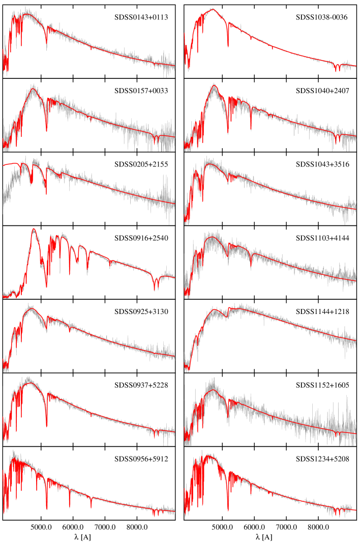
Figure 4: Observed spectra (light grey) and theoretical models (dark/red lines). Both spectra were convolved with a Gaussian with 3Å FWHM corresponding to the resolution of the SDSS spectra. The vertical axis is the flux $F_{\lambda}$ on a linear scale, with zero at the bottom.

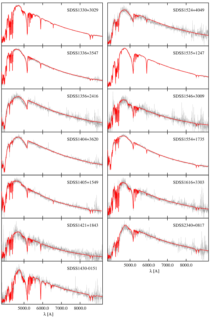
Figure 5: The same as Fig. 4 for the second half of the sample.

The Mg i/Mg ii resonance lines are predicted to be extremely strong, and it is well known that the simple impact approximation fails to reproduce the spectra in detail (Zeidler-KT et al. 1986). Potential energy curves for the MgII-He system were calculated by Monteiro et al. (1986), but are not available in tabular form in the literature. Since no ultraviolet spectra exist for our objects, a comparison with observations is not currently possible.

In order to study the effect of stronger blanketing, we have increased the neutral broadening constant $\Gamma_{6}$ for the Mg ii resonance lines by a factor of 10, which was shown by Zeidler-KT et al. (1986) to produce a line consistent with the Mg abundance derived from the optical spectrum. The resulting two-color diagram is shown in the lower panel in Fig. 3. The new sequence is a better fit to the observations, although the blanketing is still underestimated at the hot end of the sequences.

Since metals not observable in the optical spectra might contribute to the free electrons as well as to the absorption, we made a few test calculations. We added the elements C, O, Al, Si, P, S, Sc, V, Mn, Co, Ni, Cu, and Zn with abundance ratios relative to Mg taken from Klein et al. (2010), if observed in GD40, or with solar ratios otherwise. In another test series we used only the observed metals, but added 372 bound-free cross sections, mostly from Fe i. These test models showed no significant differences in the optical spectra and we therefore used only the identified elements in the analysis of the sample. The only exception is hydrogen, for which $\log$[H/He] = $-4$ (number abundances) was used unless otherwise noted in Table 3. This is a fairly typical value in the cooler objects of the Dufour et al. (2007) sample. It is also the upper limit in our spectra with higher signal-to-noise ratios, and a further reduction does not change the models anymore, since the electrons come predominantly from the metals.

As the next step we used the theoretical $ugriz$ magnitudes for both sequences (with nominal broadening constants) to estimate an effective temperature for all objects in the sample using a $\chi^{2}$ minimization. The second parameter in the fitting procedure was a number set to 1 for one sequence and 0 for the other. This allowed for an approximate interpolation between the two sets of abundances. The resulting temperature is given in Table 3 as $T_{\mathrm{eff}}$(phot) in the second column. Assuming that $\log\leavevmode\nobreak\ g$ = 8, this fitting procedure also gives a photometric distance. More than half of our sample are closer than 100 pc, and all closer than 200 pc. Interstellar reddening should not be important, compared to the other sources of uncertainty, and was neglected in our fits.

3.3 Spectral fitting

We used the temperature of the grid point closest to the best-fit photometric temperature as a starting value in the analysis of the individual objects. The abundances were varied, following a visual comparison of observed and theoretical spectrum. A small grid with $T_{\mathrm{eff}}$ 100-300 K above and below the current best value was calculated and theoretical SDSS colors for these models compared to the observed ones. Most weight was given to the most accurate colors, i.e. $g-r$ and $r-i$. This procedure was iterated, until a reasonable fit was achieved to the spectrum and the colors. $g-r$, $r-i$, and $i-z$ were usually reproduced by the final model within 1-2 $\sigma$; for $u-g$ the error was often (not always) larger (see Table 4), because of missing absorption in the $u$ region. In the higher quality spectra we could additionally use the ionization equilibrium of calcium to determine the temperature. In a few cases the final temperature differs by several 100 K from the photometric starting value, because two objects with similar colors in the intermediate range of Fig. 3 can have very different temperatures, depending on the details of the metal contamination. Figures for all spectra with the fits are displayed in Fig.4 and Fig.5.

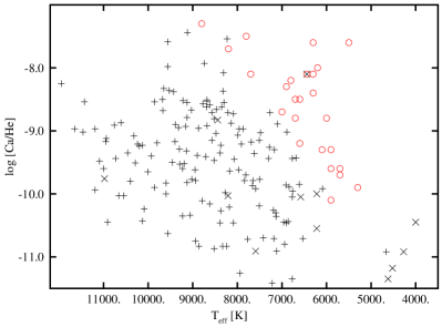
Figure 6: Calcium abundances from Dufour et al. (2007) as displayed in their Fig. 9, with our present results added. Crosses are for objects found in the SDSS, x for objects from the Bergeron et al. (2001) sample, with parameters redetermined by Dufour et al. (2007). Our new results are the (red) open circles.

4 Results

The results for $T_{\mathrm{eff}}$ and the abundances of the observed elements are given in Table 3. The objects of our sample form a natural extension of the DZ temperature sequence studied by Dufour et al. (2007). We reproduce their results of the Ca/He abundances as a function of $T_{\mathrm{eff}}$ in Fig. 6, with our results added as red open circles. The new DZ stars discovered here nicely fill in the gap which was apparent in the the Dufour et al. sample between 5500 and 8500 K at higher abundances, $\log$[Ca/He] = $-$8 to $-$10. In fact, our new sample of DZ white dwarfs provides several more objects at very large Ca/He around 6000 K, occupied up to now by the lonely G165-7. The fact that our sample does not include objects with low Ca/He abundances is likely a result of our selection procedure.

4.1 Error estimates

The $\chi^{2}$ fitting of the photometry described above gives formal errors for the effective temperatures in the range from 50 to 800 K. These are, however, not meaningful at all, as the metal abundances vary considerably from object to object, and differ generally from those used for the two sequences of our model grid. The iterative procedure used to determine individual parameters does not lead to formal error estimates. From the visual inspection we find that the fit gets noticeable worse for a change of 150 K, if the spectrum has a good signal-to-noise ratio (S/N), as well as many clear spectral features, in particular lines of Ca i and Ca ii. We hence adopt 150 K as our error estimate for the best cases, and estimate an uncertainty of 300 K for the lowest S/N objects (where the surface gravity is always fixed at the canonical value of $\log\leavevmode\nobreak\ g$ = 8).

If the temperature and gravity are fixed and their errors neglected, the uncertainties of the abundances are estimated at 0.1-0.2 dex for Mg, Ca, and Na, and 0.2-0.3 dex for Fe, Ti, Cr. If possible errors of $T_{\mathrm{eff}}$ and variations of surface gravity are included, the abundance errors can probably be up to twice these values in the worst case.

The comparison of observed and calculated $u-g$ colors shows that in most cases our models are still missing absorption near 3500 Å. In our simulation with enhanced Mg ii broadening constant we found that the model flux is enhanced over the whole observed optical range. However, the slope of the continuum and the spectral features do not change significantly. We are therefore confident that this problem does not add a larger uncertainty to the derived abundances.

Table 5: Depth of the convection zone and diffusion time scales

SDSS	q	$T_{\mathrm{eff}}$	Na	Mg	Ca	Ti	Cr	Fe
		[K]
0143+0113	$-$5.3184	6600	5.908	5.916	5.840	5.802	5.824	5.805
0157+0033	$-$5.4374	6300	5.820	5.833	5.736	5.713	5.718	5.698
0916+2540	$-$5.6914	5500	5.633	5.654	5.530	5.517	5.496	5.472
0925+3130	$-$5.4124	5900	5.879	5.896	5.799	5.790	5.789	5.769
0937+5228	$-$5.3260	6900	5.903	5.906	5.828	5.781	5.798	5.783
0956+5912	$-$5.2882	8800	5.972	5.957	5.872	5.808	5.802	5.810
1038$-$0036	$-$5.1065	8200	6.069	6.080	6.014	5.957	5.938	5.952
1040+2407	$-$5.4839	6200	5.774	5.788	5.684	5.668	5.667	5.646
1043+3516	$-$5.4041	5900	5.885	5.902	5.806	5.797	5.797	5.777
1103+4144	$-$5.4381	5700	5.870	5.890	5.789	5.788	5.779	5.757
1144+1218	$-$5.4411	5300	5.918	5.943	5.841	5.852	5.835	5.810
1152+1605	$-$5.3484	6600	5.894	5.902	5.820	5.782	5.803	5.782
1234+5208	$-$5.2821	7800	5.961	5.946	5.867	5.808	5.811	5.812
1330+3029	$-$5.4610	6440	5.799	5.810	5.706	5.679	5.683	5.662
1336+3547	$-$5.3139	6700	5.924	5.930	5.853	5.811	5.831	5.813
1356+2416	$-$5.3667	6100	5.903	5.918	5.830	5.811	5.819	5.800
1404+3620	$-$5.3800	5900	5.907	5.923	5.832	5.822	5.825	5.805
1405+1549	$-$5.1901	7700	6.026	6.016	5.950	5.893	5.888	5.890
1421+1843	$-$5.3542	6800	5.879	5.885	5.802	5.760	5.779	5.760
1430$-$0151	$-$5.5399	6300	5.734	5.748	5.634	5.616	5.611	5.589
1524+4049	$-$5.4519	5700	5.859	5.878	5.776	5.774	5.764	5.742
1535+1247	$-$5.4688	6000	5.803	5.819	5.717	5.707	5.703	5.682
1546+3009	$-$5.3588	6700	5.876	5.884	5.801	5.761	5.781	5.761
1554+1734	$-$5.2442	7000	5.978	5.973	5.908	5.856	5.870	5.864
1616+3303	$-$5.3819	6700	5.862	5.870	5.782	5.743	5.762	5.740
2340+0817	$-$5.4007	6300	5.858	5.870	5.779	5.754	5.762	5.742

4.2 Notes for individual objects

SDSS0157+0033: The Mg i triplet lines seem to be split and shifted, suggesting a noticeable magnetic field for this white dwarf. Higher S/N data are needed to confirm this hypothesis.

SDSS0205+2155: This is a DQ with Swan bands of the C₂ molecule. From comparison with a grid of DQ models we estimate an effective temperature of about 6000 K, and $\log$ [C/He] = $-$7.0. The decrease of the flux at the blue end may be due to calcium and possibly iron, which is an interesting possibility, since the current explanation for the DQ stars is dredge-up of carbon from deeper layers (Koester et al. 1982; Pelletier et al. 1986). We estimate that the Ca abundance would need to be around $\log$[Ca/He] = $-10.0$ to $-10.5$, but this is pure speculation at the moment.

SDSS0937+5228: This is a previously known white dwarf (WD0933+526), first identified as a DZ by Harris et al. (2003).

SDSS0956+5912: Dufour et al. (2007) find $T_{\mathrm{eff}}$ = 8230 K for this star, whereas we find a somewhat higher temperature from the SDSS photometry, continuum slope as well as blue flux. Our Ca abundance is also higher by about a factor two.

SDSS1038$-$0036: Our temperature is significantly higher than the 6770 K found by Dufour et al. (2007). As can be seen in their Fig. 7, the Ca ii lines near 8600 Å are much too weak in the model. It seems that a higher temperature is a better fit. The spectrum from DR7 shows unexplained features near 4720 and 4865 Å; we have used the reduction of DR4 for the same spectrum, where the features are absent.

SDSS1144+1218: The model fits the photometry very well, but the slope and absolute scale of the observed spectrum disagree. We consider this to be a calibration problem of the spectrum and the model in Fig 5 is adjusted with a linear correction.

SDSS1152+1605: Although the spectrum is very noisy there are some indications of possible Zeeman splitting in the stronger lines.

SDSS1330+3029: This star is also known as WD 1328+307 and G 165-7. It was analyzed by Dufour et al. (2006) who found it to be a weakly magnetic ($\approx 650$kG) DZ white dwarf with Zeeman splitting in lines of Ca, Na, and Fe. We used their parameters $T_{\mathrm{eff}}$ and $\log\leavevmode\nobreak\ g$, as well as their abundances and calculated a model without considering a magnetic field. As expected, the lines are slightly weaker and narrower in our model, due to the absence of the splitting, but otherwise it agrees very well with their results.

SDSS1404+3620: The photometric temperature is very likely too high. The continuum slope and Ca i/Ca ii ionization demand a much lower $T_{\mathrm{eff}}$, which we have adopted here. The theoretical colors from the final model agree with the observations.

SDSS1535+1247: This is a known white dwarf (WD 1532+129, G137-24), which was classified as DZ by Kawka et al. (2004). Because the spectrum is similar to that of G165-7, they adopted the model of Wehrse & Liebert (1980) for that star with $T_{\mathrm{eff}}$ = 7500 K and found metal abundances of $\approx 1/100$ solar. They note, however, that a fit to the $VJH$ photometry results in $T_{\mathrm{eff}}$ = 6000$\pm$400 K. The $u-g$ and $g-r$ colors are similar to SDSS1330+3029, yet the slope of the spectra is quite different. Also, adding the $i$ and $z$ magnitude for the photospheric fit results in significantly lower temperature. The best compromise using the resonance and excited lines from the two ionization stages is $T_{\mathrm{eff}}$ = 6000 K, in agreement with the photometric result of Kawka et al. (2004). The theoretical $griz$ photometry for the final model agrees well with the observations (Table 4).

SDSS1546+3009: This object may be weakly magnetic, with splittings and shifts apparent in many metal lines. A higher S/N spectrum is needed for confirmation.

5 Element abundances, diffusion, and accretion

Heavy elements in a helium-dominated atmosphere will sink out of the outer, homogeneously mixed convection zone into deeper layers. The abundance observed depends on the interplay of accretion from the outside and diffusion at the bottom of the convection zone. These diffusion time scales can be calculated for all objects using the methods and input physics as described in Koester & Wilken (2006) and Koester (2009). The data are collected in Table 5.

The size of the convection zone, and the diffusion time scales depend on the effective temperature, which determines the stellar structure. In addition it depends on the metal composition of the atmosphere, because the atmospheric data at Rosseland optical depth 50 are used as outer boundary conditions for the envelope calculations. However, the total range of time scales over all objects and all elements only varies within a factor of $\approx 4$, from $3\,10^{5}$ to $1.2\,10^{6}$ years.

As discussed in Koester (2009), the interpretation of observed abundances, and their relation to the abundances in the accreted material depends on the identification of the current phase within the accretion/diffusion scenario: initial accretion, steady state, or final decline. Except for the case of hotter DAZ, with diffusion time scales of a few years or less, we generally do not know in which phase we observe the star. The currently favored source for the accreted matter is a dusty debris disk, formed by the tidal disruption of planetary rocky material. The lifetime of such a debris disk is highly uncertain; estimates put it around $1.5\,10^{5}$ yrs (Jura 2008; Kilic et al. 2008). If the lifetime is really that short, the steady state phase would never be reached for the cool DZ analyzed here. The observable abundances would be close to the accreted abundances during the initial accretion phase. If the accretion rate declines exponentially, this abundance pattern could persist for a longer period. If the accretion is switched off abruptly, the element abundances would diverge, according to their diffusion time scales.

The differences between the time scales of the four elements Mg, Na, Ca, Fe, which are observed in most objects, are at most a factor of 1.4. Given the relatively large differences between the diffusion time scales of Mg and Fe, is possible to attribute the scatter of the Fe/Mg ratio to differences in the time since the accretion episode? Let us assume for a moment that all objects have reached similar abundances when the accretion stops. The observed range in Mg abundances of 2.7 dex would, under this assumption, be due to an exponential decline for a duration of 6.22 $\tau$(Mg). During this time the Mg/Fe ratio would change by a factor of 12 or 1.1 dex, and we would expect a correlation between Mg abundance and the Fe/Mg ratio. This model is obviously a strong oversimplification, but at least in a statistical sense it might be true that objects with lower overall metal abundance might have spent more time since the accretion stopped. Is such an effect observable?

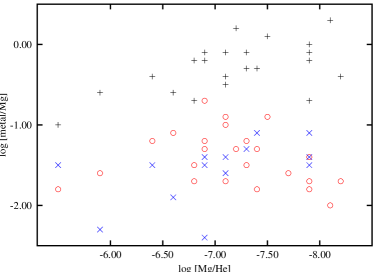
Figure 7: Ca/Mg (red circles), Fe/Mg (black crosses), and Na/Mg (blue x) as a function of the magnesium abundance.

Fig. 7 shows the comparison for the Na/Mg, Ca/Mg, and Fe/Mg ratios. There is no evolution visible in the first two ratios. For Na/Mg this is expected, since the diffusion time scales are very similar and the ratio should always stay close to the accretion ratio. This would imply that the Na/Mg ratio in the accreted material can vary by much more than a factor of ten.

If anything, the Fe/Mg ratio shows an increase, in spite of the shorter time scales of iron. This means that the Mg abundance cannot be interpreted as an indicator of time since accretion; more likely the accretion reaches different values in different objects. The variation by a factor of ten in the Fe/Mg ratio could then be explained by subsequent diffusion.

The above considerations are rather speculative and need to be taken with a grain of salt. Abundance errors in individual objects could add up to 0.5 dex, and the theoretical diffusion time scales use several approximations (Koester 2009) – we cannot exclude that the uncertainties are as high as a factor of 1.5. Because the time scales for the different elements given in Table 5 are very similar, such small changes could even invert the trends discussed above.

Table 6: Average logarithmic abundance ratios for Fe/Mg, Ca/Mg, Na/Mg, and Na/Ca

Data	[Fe/Mg]	[Ca/Mg]	[Na/Mg]	[Na/Ca]
average	$-$0.35	$-$1.42	$-$1.56	$-$0.19
$\sigma$(mean)	0.06	0.06	0.09	0.08
$\sigma$(distribution)	0.38	0.33	0.37	0.58
bulk Earth	$-$0.13	$-$1.21	$-$1.77	$-$0.56
solar	$-$0.10	$-$1.26	$-$1.36	$-$0.10

An alternative interpretation could be to assume that the metal ratios are all still close to the accreted, assumed to be similar in all objects, and that the observed distribution is caused by uncertainties of the abundances and atmospheric parameters (e.g. $\log\leavevmode\nobreak\ g$). Table 6 collects relevant data for mean values and distributions of the metal-to-Mg abundance ratios. The width of the distributions could be completely explained, assuming typical errors of 0.15 dex for Mg, and 0.25 dex for Fe, Ca, and Na. In view of the error discussion above this is not implausible.

6 Conclusions

We have identified 26 DZ and one DQ stars across and below the main sequence in the $u-g$ vs. $g-r$ SDSS two-color diagram, most of which are new detections. A search routine tailored to the specific spectral features observed in these DZ was needed to avoid the confusion by the much more numerous main sequence stars and QSOs in this region. From our analysis with theoretical model atmospheres, which uses newly developed line profiles for the strongly broadened Ca and Mg lines, we determined the white dwarf temperatures and abundances for the polluting elements Ca, Mg, Fe, Na, and in a few cases Cr and Ti. The temperatures and abundances show that these objects form a sequence which continues that of the hotter DZs in the sample of Dufour et al. (2007). The new objects fill the deficiency of objects with $T_{\mathrm{eff}}$$\la$ 8000 K at high Ca/He abundances, which was apparent in that work. We do not find new low-abundance DZ, which is most likely a consequence of the design of our search algorithm.

Very little is known for these DZ regarding their current phase in the accretion/diffusion scenario. However, if the accretion is, or was, from a circumstellar dust disk, it is unlikely that a steady state phase occurs, since the diffusion time scales are of the same order as the expected lifetime of such a disk. Because the diffusion time scales of the observed elements are very similar, we might expect that the metal-to-metal ratios are not too far from those in the accreted matter, and we compare the average values of these elements in the bulk Earth (Allègre et al. 1995) and the Sun (Asplund et al. 2009) in Table 6. The average abundance ratios found for our DZ sample are similar to those of both bulk Earth and the Sun, with the Na/Ca ratio slightly favoring the solar abundance ratio.

An important element for a distinction between different sources would be carbon, which is not detected in our sample. This element is about a factor of 100 under-abundant in the bulk Earth, compared to the Sun and the interstellar medium. The DQ star SDSS0205+2155 demonstrates that $\log$[C/He] = $-$7 produces clearly visible Swan bands. However, with the metal pollution in the other objects, the pressure and the transparency in the atmosphere are lower (due to more free electrons), and the typical upper limits are $\log\mathrm{[C/He]}=-5.5$ to $-6.0$, which is too high to distinguish between bulk Earth and solar/ISM carbon abundances.

Another critical element for all possible explanations is hydrogen. We note that in all objects the abundance of hydrogen relative to the metals is less than the solar value, even in the one case where it is detected. This is consistent with accretion of predominantly volatile-depleted material, since hydrogen accreted from the interstellar matter or from circumstellar water/ice would stay in the convection zone and can only accumulate with time.

In the case of the DBZ star GD40, Klein et al. (2010) were able to deduce very detailed conclusions from a comparison of photospheric abundances with those of various solar system bodies. The abundance ratios we obtain here roughly follow that of the bulk Earth. However, the remaining uncertainties of surface gravity, abundances, and time since the last accretion event do not allow us to draw any further conclusions in the present study. High resolution, high S/N observations and extending the spectral coverage at least to 3200 Å, or better to 2700 Å (to cover the Mg ii/Mg i resonance lines) are needed to refine the element abundances and detect the very crucial element silicon, and if possible carbon and oxygen.

We can, however, estimate a lower limit for the total accreted mass based on the available data for the convection zone. For SDSS0956+5912, which has the highest metal pollution, we find a total mass for the observed metals Mg, Ca, Fe, Na of $1.5\,10^{23}$g. Adding oxygen with the same ratio to Mg as in GD40 (Klein et al. 2010) this number becomes $4.8\,10^{23}$g, even more than in the extremely heavily polluted SDSS0738+1835 (Dufour et al. 2010). The total amount of H in the convection zone is $1.0\,10^{24}$g. For SDSS1144+1218, which has the lowest abundances, these numbers are $3.2\,10^{20}$g (observed metals), and $7.9\,10^{20}$g (including oxygen). These masses span the range of the most massive asteroids in our own planetary system. These are the absolute minimum of the accreted masses – depending on how long ago the accretion ended, these masses can be at least two orders of magnitude larger, which will require minor planets much larger than known in the Solar system. Another open question, recently discussed by Farihi et al. (2011) in the context of G77-50, a DAZ of similar low temperature, is how such a very massive asteroid is suddenly driven into its host star from an orbit apparently stable over the past 5 Gyrs.

References

- Abazajian et al. (2009) Abazajian, K. N., Adelman-McCarthy, J. K., Agüeros, M. A., et al. 2009, 182, 543
- Allard & Kielkopf (1982) Allard, N. & Kielkopf, J. 1982, Reviews of Modern Physics, 54, 1103
- Allard et al. (2003) Allard, N. F., Allard, F., Hauschildt, P. H., Kielkopf, J. F., & Machin, L. 2003, A&A, 411, L473
- Allègre et al. (1995) Allègre, C. J., Poirier, J., Humler, E., & Hofmann, A. W. 1995, Earth and Planetary Science Letters, 134, 515
- Asplund et al. (2009) Asplund, M., Grevesse, N., Sauval, A. J., & Scott, P. 2009, ARA&A, 47, 481
- Bergeron et al. (2001) Bergeron, P., Leggett, S. K., & Ruiz, M. T. 2001, ApJS, 133, 413
- Czuchaj et al. (1996) Czuchaj, E., Rebentrost, F., Stoll, H., & Preuss, H. 1996, Chemical Physics, 207, 51
- Debes & Sigurdsson (2002) Debes, J. H. & Sigurdsson, S. 2002, ApJ, 572, 556
- Dufour et al. (2007) Dufour, P., Bergeron, P., Liebert, J., et al. 2007, ApJ, 663, 1291
- Dufour et al. (2006) Dufour, P., Bergeron, P., Schmidt, G. D., et al. 2006, ApJ, 651, 1112
- Dufour et al. (2010) Dufour, P., Kilic, M., Fontaine, G., et al. 2010, ApJ, 719, 803
- Dupuis et al. (1992) Dupuis, J., Fontaine, G., Pelletier, C., & Wesemael, F. 1992, ApJS, 82, 505
- Dupuis et al. (1993a) Dupuis, J., Fontaine, G., Pelletier, C., & Wesemael, F. 1993a, ApJS, 84, 73
- Dupuis et al. (1993b) Dupuis, J., Fontaine, G., & Wesemael, F. 1993b, ApJS, 87, 345
- Farihi et al. (2010a) Farihi, J., Barstow, M. A., Redfield, S., Dufour, P., & Hambly, N. C. 2010a, MNRAS, 404, 2123
- Farihi et al. (2011) Farihi, J., Dufour, P., Napiwotzki, R., & Koester, D. 2011, MNRAS, 358, ArXiv e-prints 1101.2203
- Farihi et al. (2010b) Farihi, J., Jura, M., Lee, J., & Zuckerman, B. 2010b, ApJ, 714, 1386
- Farihi et al. (2009) Farihi, J., Jura, M., & Zuckerman, B. 2009, ApJ, 694, 805
- Gänsicke et al. (2008) Gänsicke, B. T., Koester, D., Marsh, T. R., Rebassa-Mansergas, A., & Southworth, J. 2008, MNRAS, 391, L103
- Gänsicke et al. (2007) Gänsicke, B. T., Marsh, T. R., & Southworth, J. 2007, MNRAS, 380, L35
- Gänsicke et al. (2006) Gänsicke, B. T., Marsh, T. R., Southworth, J., & Rebassa-Mansergas, A. 2006, Science, 314, 1908
- Gänsicke et al. (2010) Gänsicke, B. T., Koester, D., Girven, J., Marsh, T. R., & Steeghs, D. 2010, Science, 327, 188
- Harris et al. (2003) Harris, H. C., Liebert, J., Kleinman, S. J., et al. 2003, AJ, 126, 1023
- Holberg et al. (1997) Holberg, J. B., Barstow, M. A., & Green, E. M. 1997, ApJ, 474, L127
- Jura (2003) Jura, M. 2003, ApJ, 584, L91
- Jura (2006) Jura, M. 2006, ApJ, 653, 613
- Jura (2008) Jura, M. 2008, AJ, 135, 1785
- Kawka et al. (2004) Kawka, A., Vennes, S., & Thorstensen, J. R. 2004, AJ, 127, 1702
- Kilic et al. (2008) Kilic, M., Farihi, J., Nitta, A., & Leggett, S. K. 2008, AJ, 136, 111
- Klein et al. (2010) Klein, B., Jura, M., Koester, D., Zuckerman, B., & Melis, C. 2010, ApJ, 709, 950
- Koester (2009) Koester, D. 2009, A&A, 498, 517
- Koester et al. (1997) Koester, D., Provencal, J., & Shipmann, H. L. 1997, A&A, 320, L57
- Koester et al. (1982) Koester, D., Weidemann, V., & Zeidler-KT, E. M. 1982, A&A, 116, 147
- Koester & Wilken (2006) Koester, D. & Wilken, D. 2006, A&A, 453, 1051
- Kuiper (1941) Kuiper, G. P. 1941, PASP, 53, 248
- Kupka et al. (1999) Kupka, F., Piskunov, N., Ryabchikova, T. A., Stempels, H. C., & Weiss, W. W. 1999, A&AS, 138, 119
- Kupka et al. (2000) Kupka, F. G., Ryabchikova, T. A., Piskunov, N. E., Stempels, H. C., & Weiss, W. W. 2000, Baltic Astronomy, 9, 590
- Monteiro et al. (1986) Monteiro, T. S., Cooper, I. L., Dickinson, A. S., & Lewis, E. L. 1986, Journal of Physics B Atomic Molecular Physics, 19, 4087
- Pelletier et al. (1986) Pelletier, C., Fontaine, G., Wesemael, F., Michaud, G., & Wegner, G. 1986, ApJ, 307, 242
- Piskunov et al. (1995) Piskunov, N. E., Kupka, F., Ryabchikova, T. A., Weiss, W. W., & Jeffery, C. S. 1995, A&AS, 112, 525
- Richards et al. (2002) Richards, G. T., Fan, X., Newberg, H. J., et al. 2002, 123, 2945
- Ryabchikova et al. (1997) Ryabchikova, T. A., Piskunov, N. E., Kupka, F., & Weiss, W. W. 1997, Baltic Astronomy, 6, 244
- Sion et al. (2009) Sion, E. M., Holberg, J. B., Oswalt, T. D., McCook, G. P., & Wasatonic, R. 2009, 138, 1681
- Unsöld (1968) Unsöld, A. 1968, Physik der Sternatmosphären (Berlin: Springer-Verlag)
- von Hippel et al. (2007) von Hippel, T., Kuchner, M. J., Kilic, M., Mullally, F., & Reach, W. T. 2007, ApJ, 662, 544
- Walkup et al. (1984) Walkup, R., Stewart, B., & Pritchard, D. E. 1984, Phys. Rev. A, 29, 169
- Wehrse & Liebert (1980) Wehrse, R. & Liebert, J. 1980, A&A, 86, 139
- Zeidler-KT et al. (1986) Zeidler-KT, E. M., Weidemann, V., & Koester, D. 1986, A&A, 155, 356