Spatial fluctuations in transient creep deformation

Abstract

We study the spatial fluctuations of transient creep deformation of materials as a function of time, both by Digital Image Correlation (DIC) measurements of paper samples and by numerical simulations of a crystal plasticity or discrete dislocation dynamics model. This model has a jamming or yielding phase transition, around which power-law or Andrade creep is found. During primary creep, the relative strength of the strain rate fluctuations increases with time in both cases - the spatially averaged creep rate obeys the Andrade law $\epsilon_{t}\sim t^{-0.7}$, while the time dependence of the spatial fluctuations of the local creep rates is given by $\Delta\epsilon_{t}\sim t^{-0.5}$. A similar scaling for the fluctuations is found in the logarithmic creep regime that is typically observed for lower applied stresses. We review briefly some classical theories of Andrade creep from the point of view of such spatial fluctuations. We consider these phenomenological, time-dependent creep laws in terms of a description based on a non-equilibrium phase transition separating evolving and frozen states of the system when the externally applied load is varied. Such an interpretation is discussed further by the data collapse of the local deformations in the spirit of absorbing state/depinning phase transitions, as well as deformation-deformation correlations and the width of the cumulative strain distributions. The results are also compared with the order parameter fluctuations observed close to the depinning transition of the 2$d$ Linear Interface Model or the quenched Edwards-Wilkinson equation.

1 Introduction

Recent research has highlighted the importance of fluctuations and heterogeneous response in the behavior of materials. The central issue is that the ”rheological” laws that describe what happens to a sample under loading are coarse-grained from the microscopic behavior. From this viewpoint, it is then imperative to understand what are the origins of various phenomena in this field, and to grasp the consequences for e.g. materials science. The main emphasis in what follows starts from the phenomenological primary creep law, which states that the deformation rate decays in time as a power law, as $\frac{d\epsilon(t)}{dt}\equiv\epsilon_{t}\sim t^{-\theta}$. The particular value $2/3$ is coined as Andrade’s creep, originating from 1910 and its theoretical roots are still under a debate [1, 2, 3].

Crystalline materials deform plastically via the motion of dislocations. Some time ago, it was shown that two-dimensional dislocation assemblies exhibit a yielding transition [4]. This is a non-equilibrium phase transition separating a state which is asymptotically quiescent from an active (yielding) one as the control parameter, external stress, is varied. The order parameter - the strain rate - seems to exhibit a second order phase transition at the critical yield stress $\sigma_{c}$. Since it was shown that such simple materials science/physics models exhibit critical phenomena the research related to the statistical mechanics of crystal plasticity has exploded to various directions including coarse-grained models [5], studies of the properties of the transition [6], experimental signatures such as crackling noise as acoustic emission [7, 8] and in stress-strain curves [9], characterization of the deformation structures [10], surface patterning [11], and three-dimensional studies [12].

However, e.g. Andrade creep is a concept that has been demonstrated in non-crystalline materials from rocks to composites [13]. To outline some particular cases, the deformation of amorphous metallic glasses has recently become an active field of its own, and there as well collective phenomena are now being discussed and studied [14, 15, 16]. In that case, and in the physics of the jamming of granular assemblies [17, 18, 19] the origins of the intermittent deformation are being studied with concepts that are focused upon such materials, such as ”shear transformation zones” or the ”cage effect” [20]. Whatever the microscopic physics, it is an important question of what kind of signatures can be actually found in experiments on deformation on the coarse-grained scale. In this work, we tackle this issue by studying the spatiotemporal characteristics of creep deformation, that is to say the response of material samples to a constant load. As noted above, there are indications that collective phenomena might be of decisive importance. A short account of the results has been published recently in [2].

The questions that are of primary interest are: i) what kind of fluctuations can be seen in the creep of experimental samples and idealized dislocation assemblies, by computer simulation? ii) do these show universality beyond the models that would be appropriate for the material at hand? iii) what kind of correlations and fluctuations ensue, for both the ”order parameter” (creep rate, for the Andrade creep at least) and the integrated order parameter, i.e. the total creep strain? The outcomes for such questions present a challenge for the statistical physics of materials science. There are a few theories relevant for the creep deformation of materials. For the particular case of dislocation systems, it appears that modified versions of depinning (DP) transitions (of elastic manifolds in random media) or absorbing state (AS) phase transitions might be in order [5]. The fundamental problem is how to coarse-grain such a theory from assemblies of individual topological defects [21]; however the DP/AS paradigm offers suggestions about what to look for in the empirical data whether from simulations of a model that is supposed to adhere to such a phase transition picture, or from the experiments.

In what follows, simple paper samples are found to exhibit a primary creep regime characterized by the power law decay of the average creep strain rate, $\epsilon_{t}\sim t^{-0.7}$, analogously to the Andrade law valid for many materials ranging from soft metals to ordinary paper [1, 22]. The spatial variations of the strain rate are studied by the digital image correlation method, and are found to be characterized by a power law time dependence of the standard deviation of the local strain rates, $\Delta\epsilon_{t}\sim t^{-0.5}$, during the Andrade’s creep. Thus, the magnitude of the fluctuations of the strain rate decays slower with time than the average creep rate, implying that fluctuations become more important in relative terms with time. This feature persists in the logarithmic creep. Similar behavior is observed in a discrete dislocation dynamics or crystal plasticity model, which is known to exhibit a non-equilibrium jamming/yielding phase transition at a critical value of the applied external shear stress. These results are further compared with simulations of the two-dimensional Linear Interface Model (LIM)/quenched Edwards-Wilkinson (qEW) equation close to the depinning transition. Such a simple 2$d$ model provides a convenient “benchmark” system with a simple AS/DP transition where the relevant phenomena can be studied in a transparent manner.

The paper is organized as follows: In the next Section we discuss details of the numerical simulations of the discrete dislocation dynamics model, as well as the experimental setup and measurement methods of the paper deformation experiments. In Section 3 we present the results of both the numerical simulations, including also simulations of the LIM/qEW case, and experiments. These are then discussed both from the point of view of classical theories of Andrade creep in dislocation systems, as well as by considering a picture emerging from interpreting the creep deformation as a process occurring close to a non-equilibrium second order phase transition. Section 4 finishes the paper with conclusions.

2 Details of simulations and experiments

2.1 Dislocation model simulations

The discrete dislocation dynamics (DDD) simulations are performed by means of a two-dimensional model of shear deformation with point-like edge dislocations (See [4] or e.g. [23]) . These point dislocations glide under the influence of the local Peach-Koehler forces or shear stresses acting on them. These are superpositions of the applied external shear stress $\sigma$ and the internal stresses $\sigma_{s}$ due to the long range anisotropic stress fields

$$\sigma_{s}({\bf r})=Dbx\frac{(x^{2}-y^{2})}{(x^{2}+y^{2})^{2}}$$ (1)

of all the other dislocations in the system. Here $D=\mu/2\pi(1-\nu)$, with $\mu$ the shear modulus and $\nu$ the Poisson ratio of the material. $b$ is the magnitude of the Burgers vector of the dislocations. Such a system can also be thought to represent a two-dimensional cross section of a three-dimensional assembly of straight parallel edge dislocations. Only a single slip system is considered (i.e. dislocation glide is allowed in the $x$-direction only within the $xy$ plane of the system), and no dislocation climb is taken into account. The equations of motion are taken to be overdamped, such that

$$\frac{\chi_{d}^{-1}v_{n}}{b}=s_{n}b\left[\sum_{m\neq n}s_{m}\sigma_{s}({\bf r}_{nm})+\sigma\right],$$ (2)

where $v_{n}$ is the velocity of the $n$th dislocation, $\chi_{d}$ refers to the dislocation mobility, $s_{n}$ is the sign of the Burgers vector of the $n$th dislocation, and $\sigma$ is the external shear stress.

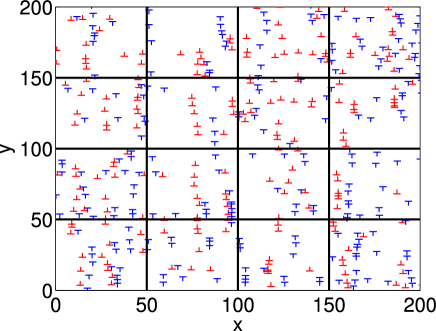
Figure 1: A snapshot from the dislocation system. A two-dimensional system of discrete edge dislocations subject to an external shear stress $\sigma$ close to the critical value $\sigma_{c}\approx 0.025$, showing also the division into boxes of $l=50b$. The colors (red and blue) indicate the sign of the Burgers vector of the dislocations. Only glide motion of dislocations along $x$ direction is considered for simplicity. We study the spatial fluctuations of the strain rate by dividing the system into boxes of linear size $l$, and defining the local strain rates over some time interval $\Delta t$, see Equations (5) and (6).

In the simulations, dimensionless units are used by measuring lengths in units of $b$, times in units of $1/(\chi Db)$, and stresses in units of $D$. The stresses are computed by imposing periodic boundary conditions in both directions. The equations of motion are integrated numerically with an adaptive step size fifth order Runge-Kutta algorithm. The system is initially composed of a random arrangement of $N_{0}$ such dislocations, with Burgers vectors ${\bf b}=\pm b{\bf u}_{x}$ parallel to the glide direction (with an equal number of dislocations with the $+$ and $-$ signs). To mimic dislocation annihilation occurring in real plastically deforming crystals, two dislocations with Burgers vectors of opposite sign are removed from the system if their mutual distance is less than $2b$. The random initial configurations are first let to relax in the absence of externally applied stresses. During this initial relaxation, a significant fraction of the dislocations get annihilated, leading to a reduction of the dislocation number from the initial $N_{0}=1600$ for $L=200b$ to the range of $N=500-600$ after the relaxation. During the subsequent dynamics under the influence of an external stress $\sigma\approx\sigma_{c}$, only a small amount of further dislocation annihilations take place. Notice that the relaxation process described above before applying the external stress is essential to obtain the Andrade law: initial conditions with randomly positioned dislocations lead to a different, roughly exponential time dependence of the strain rate [24].

It is known that the DDD model exhibits a jamming or yielding phase transition, at a critical value $\sigma_{c}$ of the shear stress [25]. Below that the activity eventually stops as at absorbing state phase transitions typically. Above, in the thermodynamic limit, a finite deformation rate exists. By applying a constant external stress, for the setup described above, we find $\sigma_{c}\approx 0.025$. For an example of a dislocation configuration observed close to the jamming threshold, see Figure 1. Notice that the dislocations tend to form various metastable structures, such as dipoles and walls.

2.2 Experimental setup

The experimental setup is shown in Figures 2 and 3. The lower clamp is connected to a set of metal weights. Typical loads were around 40 N which corresponds to a stress of 13 MPa. The samples were 100 mm $\times$ 30 mm slices cut from standard office paper, loaded in the “cross-machine” direction. Relative humidity and temperature were kept in constant conditions at 30% and 22 C^∘, respectively, and the applied load was adjusted to achieve different creep times-to-failure, which generally were between 10 and 60 minutes. In the experiment, the sample is fixed between steel clamps mounted on an aluminum frame and a steel jig is used to ensure the correct alignment of the sample between the clamps. The sample is imaged during the experiment with a digital camera. A laser distance sensor is used to measure the elongation of the sample together with a digital image correlation analysis.

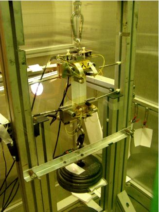
Figure 2: The setup for creep experiments. A load is attached to the lower clamp and its movement is controlled by using pneumatic cylinders. A camera was attached to the frame, and a laser distance sensor followed the movement of the lower clamp. Images were taken during the experiment at rate 0.1 Hz…1 Hz.

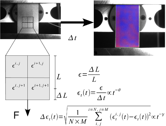
Figure 3: The experimental scenario. From a pair of digital images at a time-interval $\Delta t$, the local deformations are extracted at a grid. The strain fluctuations are measured via the time-dependent standard deviation, and compared to the mean creep rate, here in primary/Andrade creep. In the DDD simulations a similar approach is used, by subdividing the system of linear size $L$ into boxes of linear size $l$ in which the local strain rates $\epsilon_{t}^{i,j}$ are measured. A digital image of a paper sample on a scale of 40 mm². Superposed is a typical deformation grid for a time difference $\Delta t$ of 10 seconds. The color scale indicates the degree of local creep deformation (blue: small, red: large). In the background: the experimental setup. The visible speckle pattern has been printed, and designed to have a structure and contrast appropriate for the DIC method on the scale at hand. Figure reproduced from [2].

A set of experiments with a larger magnification was also made. The typical image size was about 3 mm $\times$ 4 mm and the samples were specially prepared laboratory sheets, where 5% of the fibres were treated with colour prior to fabrication or sheet making to enhance the contrast and to produce a sharp natural-type pattern. The larger magnification makes it possible to reduce the noise level, which is relative to digital image dimension, and to obtain the strain rates and their fluctuations throughout the entire experiment.

The sample was imaged during the experiment with PCO’s 1 mega pixel grayscale digital camera, SensiCam 370KL0562. The camera has a low thermal noise ratio due to the cooled CCD and 12 bit grayscale resolution. The exposure time in measurements was 200 ms. The sampling frequency of the digital imaging is in the range 0.1…1Hz.

2.3 Strain field measurement in experiments

The strain is defined on an evenly spaced grid on an image, which consists of a discrete set of points $(i,j)$ with constant spacing $\Delta d$. $j$ refers to the strain direction. From the DIC one obtains displacements on each point $\Delta y^{i,j}$ in a time interval $dt$. A spatial strain rate $\epsilon_{t}^{i,j}$ in a grid point $(i,j)$ is computed using

$$\epsilon_{t}^{i,j}=\frac{\Delta y^{i,j+l/2}-\Delta y^{i,i-l/2}}{ldt}$$ (3)

where $l$ is the length scale within which the strain is measured. The distribution $P(\epsilon_{t}^{i,j})$ ensues, which describes the strain rate evolution during the creep experiment. An example of the displacement distribution is shown in Figure 4, and the computation of the local strain rates is illustrated schematically in Figure 3.

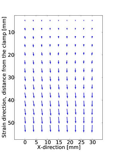
Figure 4: Vector field of absolute displacements at $t=10\,s$ in the creep experiment on paper. Vector lengths are scaled so as to just avoid an overlap and thus show the relative differences of displacement vectors. Sample time to failure $t_{c}=1549\,s$.

The starting point of the DIC algorithm is an elastic image registration algorithm [26, 27, 28]. The algorithm describes both the image and the deformation using the B-spline model. The algorithm finds the deformation function by using the multiresolution approach for the minimization, so that the image and the deformation model is refined every time the convergence is reached. The criteria for the convergence is the sum of squared differences (SSD), i.e. the deformation function is applied to the original image and the SSD is computed against the deformed image. The algorithm is described in [29]. The knots of the B-splines were defined in an evenly spaced grid, with knot spacing $h\times h$ pixels. The exact algorithm for the deformation computation is described in [29]. Knot-spacings, i.e. crates 16x16 to 64x64 pixels were used in the computations. One method to estimate the error of the displacement field is by using different crates for same image pairs: the difference of deformations was computed using two different crates and it was of the order of 0.003 pixels. As a conclusion of these tests in various experiments [2, 30] we can expect that the algorithm is able to find large continuous deformations with an accuracy of about 0.1 mm in the sample-scale imaging. The out-of-plane deformations put a limit to the accuracy, since the paper thickness is the order of 0.1 pixels in the sample scale experiments.

Note that the sampling frequency of our imaging is such that we do not expect to see the single, microscopic ”plastic” or yield events [31]. That is, our results do not reflect directly on the microscopic nature of the dynamics that leads to the fluctuations we actually measure. Thus we cannot conclude much on the elementary processes and their interactions in space and time, except in the coarse-grained sense. This is actually also quite true for the DDD model, though all the dynamics is carried out by the mobile dislocations - figuring out the causality of the intermittent dynamics is not easy. One should also point out that we measure with the technique localized strain fluctuations, which however are not a priori nor a posteriori related to any localization in the sense of the formation of “strain bands”, or “yield bands”. A separate study should be done on the possibility of observing related phenomena in the tertiary creep phase.

When defining and measuring the fluctuations of the strain-field we study only the $y$-component of the strain. This is a simplification since also transverse strains are observed. This is seen in Figure 4 where we show the vector field of absolute displacements taken from the primary creep regime of a sample whose total time to failure was $t_{c}=1549\,$s. As can be seen, the $y$-component is clearly the dominating component of deformation.

It is furthermore important to point out that the local strain (rate) fluctuations are in no obvious way connected directly to the disordered structure. Figure 3 illustrates also partly the variations in the sheet transparency, which is related to the local porosity and to the mass per unit area and its fluctuations. These are in turn correlated in a non-trivial way with the local elastic and inelastic material response.

2.4 Measuring acoustic emission and typical creep curve

The strain from an experiment together with acoustic emission (AE) events is presented in the main figure of Figure 5. The inset shows an example signal from an acoustic emission timeseries, with the events shown.

The AE measurement system consists of a piezoelectric transducer, a rectifying amplifier and works with continuous data-acquisition. The time-resolution of measurements is 10 $\mu$s and the data-acquisition is free of dead time. During the experiment we acquire bi-polar acoustic amplitudes by piezocrystal sensor, as a function of time. The transducer is attached directly to paper and no coupling agent is used. Data acquisition channel has 12-bit resolution and a sampling rate of 312 000/s. The transmission time from event origin to sensors is of the order of 5 $\mu$s. Acoustic channels are first amplified and after that saved to a hard disk. The shape of the AE pulses can change and attenuate during transmission, but that should have only a minor effect on our analysis. Post-processing (thresholding) the amplitude signal we find a discrete sequence of events with corresponding energies $E_{i}$ and arrival times $t_{i}$. Figure 5 shows that in a typical test, one observes the usual creep phases if the test is allowed to continue until final failure. The important point is that actual AE starts only close to the final failure of the sample.

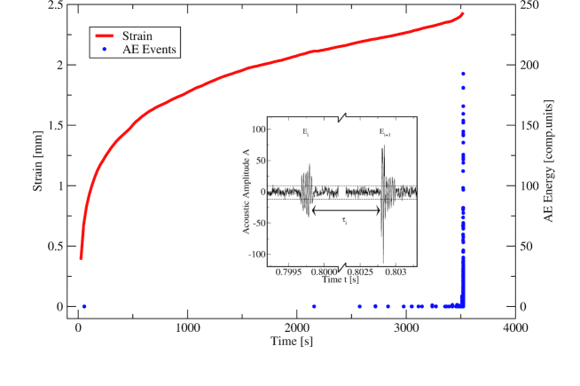
Figure 5: Typical time vs. strain curve from a creep experiment, with also the AE energy shown as a function of time. Red curve shows the total strain of the sample and the blue dots indicate acoustic emission events during the experiment, with the energy scale indicated on the right. Inset: zoom to the acoustic emission signal, where we observe two consecutive events with energies $E_{i}$ and $E_{i+1}$ greater than a given threshold and a waiting time $\tau_{i}$. This figure shows typical creep behaviour of paper, with the three phases (primary, secondary, tertiary). It also indicates the relative absence of crackling noise, that is the small number of acoustic emission events (AE) during the primary (no events) and secondary creep of the sample.

It is interesting to note that there is a large degree of variability (Figure 6) in the typical timescales of the creep process from sample to sample, but that the minimum creep rate time $t_{m}$ and the failure time $t_{c}$ are linearly related: a Monkman-Grant -like universal behavior exists such that $t_{m}\sim 0.83t_{c}$ [33, 32]. In other words, there is a degree of universality in the behavior of individual samples since the shape of the creep rate curves is such that the life-time is preceded by such a minimum around the transition to tertiary creep. The role of the strain fluctuations for the origins of the $t_{m}/t_{c}$-relation should be further investigated.

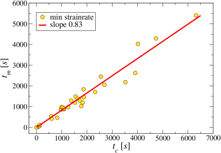
Figure 6: Time to failure vs. time to minimum of the strain rate from the experimental data. Time $t_{m}$ to the strain rate minimum is proportional to time to failure $t_{c}$. The best-fit proportionality constant indicates $t_{m}\sim 0.83t_{c}$. This is similar to the typical Monkman-Grant relation [33].

3 Results and discussion

In this section we review the main results, and discuss briefly their interpretation. At first we consider arguments for the strain rate fluctuations $\Delta\epsilon_{t}(t)\sim t^{-\gamma}$. These are in spirit related to dislocation based theoretical arguments for the Andrade law presented by Cottrell [34] and earlier by Mott [35]. We conclude that as expected these have problems with the fluctuation scaling, as they do not include collective phenomena. Then, we link the local creep statistics to scaling theories of integrated order parameter fluctuations for absorbing state/depinning phase transitions. This is analyzed both for the experimental data and the simulations, including a brief study of the order parameter fluctuations exhibited by the LIM/qEW equation close to the depinning transition.

3.1 Strain rate and fluctuations in the DDD model

In agreement with previous results [4, 36], we find that the mean strain rate for $\sigma\approx\sigma_{c}$ behaves in the relaxation phase as

$$\langle\epsilon_{t}\rangle(t)=\left\langle\frac{b}{L^{2}}\sum_{n=1}^{N}s_{n}bv_{n}(t)\right\rangle\sim t^{-\theta},$$ (4)

with $\theta\approx 2/3$, corresponding to the Andrade/primary creep law.

We then study the spatial fluctuations of the strain rate by dividing the system (see Figure 1) into boxes of linear size $l$, and defining the local strain rates over some time interval $\Delta t$ by

$$\epsilon_{t}^{i,j}(t)=\frac{b}{l^{2}}\sum_{{\bf r}_{n}\in{\mathrm{b}ox}~{}i,j}s_{n}b\left[\frac{x_{n}(t+0.5\Delta t)-x_{n}(t-0.5\Delta t)}{\Delta t}\right].$$ (5)

The possible choices for the linear box size $l$ are limited by $1/\sqrt{\rho}<l<L$, where $\rho$ is the dislocation density (and thus $1/\sqrt{\rho}$ is the mean dislocation-dislocation distance). Therefore, for $L=200b$, we consider $l=25b$, $50b$ and $100b$. There are practical limits also for $\Delta t$ values that can be used: these should be much smaller than the numerically feasible simulation times (of the order of $10^{4}-10^{5}$ time units), but also as long as possible to be able to meaningfully compare the results with experiments in which two consecutive images are separated by a “macroscopic” time. Therefore we chose to use $\Delta t=100$ in the simulations as is visible in Figure 7.

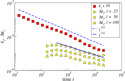
Figure 7: The Andrade’s law and the fluctuation scaling for the DDD model for three different box sizes to compute the local rates, at $\sigma\approx\sigma_{c}$. The early-time cross-over in the fluctuations is due to the fixed time-intervals of $\Delta t=100$ at which they are computed. Figure reproduced from [2].

The spatial strain rate fluctuations are quantified by the time dependence of the standard deviation of the local strain rates,

$$\Delta\epsilon_{t}(t)=\sqrt{\left(\frac{l}{L}\right)^{2}\sum_{i,j}(\epsilon_{t}^{i,j}(t)-\langle\epsilon_{t}^{i,j}(t)\rangle)^{2}}.$$ (6)

For times $t>\Delta t$, $\Delta\epsilon_{t}(t)$ is found to decay like a power law in time, $\Delta\epsilon_{t}\sim t^{-\gamma}$, with $\gamma\approx 0.5$. Thus, the magnitude of the strain rate fluctuations decays more slowly in time than the mean strain rate, implying that the role of the fluctuations becomes increasingly important with time.

3.2 Strain rate and fluctuations in the paper experiments

Similarly to the results of the DDD simulations, the experimental samples are found to exhibit a primary creep regime characterized by a power law decay of the average creep strain rate,

$$\langle\epsilon_{t}\rangle\sim t^{-0.7\pm 0.1}.$$ (7)

The spatial variations are found to be characterized by a power law time dependence of the standard deviation of the local strain rates,

$$\Delta\epsilon_{t}=\sqrt{\frac{1}{N}\sum_{i,j}(\epsilon_{t}^{i,j}(t)-\langle\epsilon_{t}^{i,j}(t)\rangle)^{2}}\sim t^{-\gamma},$$ (8)

where the fluctuation exponent $\gamma=0.55~{}\pm~{}0.1$ is found.

The magnitude of the fluctuations of the strain rate decay slower with time than the average creep rate, implying that fluctuations become more important in relative terms with time. An average over 16 samples is presented in Figure 8, and a single example is shown in Figure 9. The fluctuation scaling result was independent of the length $l$ used. In the sample scale images during creep, the fluctuation scaling was observed using $l=14...60~{}mm$. Here, the crate is the lower and the sample size the upper bound of $l$. At lower stresses, logarithmic creep is found with no signature of the Andrade phase. The DIC analysis on the magnified images shows that the relative strength of the fluctuations increase also during the logarithmic creep phase, as evidenced by Figure 10, where $l=0.3$ mm was used.

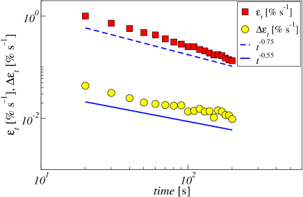
Figure 8: Average creep rate and the standard deviation of the local creep rates from the sample scale experiments. Data for a typical set of experiments, $l$ = 60mm and crate 48 $\times$ 48, and SSD = 0.1 pixels. The samples average lifetime is 800-1600 seconds. The Andrade-to-logarithmic creep transition appears to take place continuously at 150-200 seconds. The data is averaged over 16 experiments. The effective Andrade exponent is about 0.7, in the range 10 to 50 seconds, and becomes close to one (signalling the onset of logarithmic creep) above 150 seconds. Figure reproduced from [2].

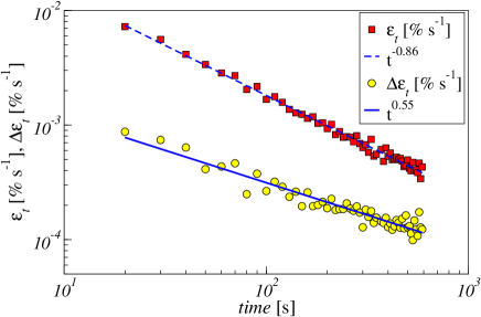
Figure 9: An example of the average creep rate and the standard deviation of a single sample. The crate is 16x16 pixels, SSD=0.05 pixels and l=3mm.

The average creep rate and the fluctuation amplitude change with time so the creep rate probability distribution (PDF) might evolve as well. Typical examples of the distributions of (the y-component of) relative strain rates are depicted if Figure 11, showing that such PDF’s become narrower but can be otherwise roughly collapsed with the expected exponent.

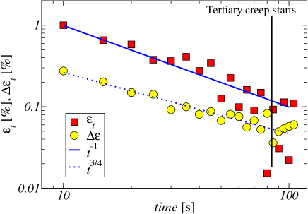
Figure 10: Experimental results from logarithmic creep using a smaller imaging area, 5 second image intervals, $l$=0.3mm, and a smaller load, showing the average creep rate and the fluctuations. The former decays faster, and at the end these two become comparable, on the observation scale. The data is an average over 9 experiments. Figure reproduced from [2].

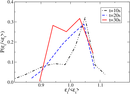
Figure 11: The scaled probability distribution functions of strain rates $\epsilon_{t}^{i,j}$ from an experiment, where the time to failure is 1038 s. The width of the distributions increases when time passes. The skewness decreases in this particular sample, but the feature is not observed in all experiments.

3.3 Local stress-fields and elastic modulus fluctuations of paper samples

The structure of paper exhibits disorder in many scales [37]. In this work we have studied fluctuations of the strain field during the creep experiment which corresponds a floc-scale and a fiber-scale. The floc-scale corresponds density fluctuations of paper sheet at scales order of 1 cm. The fiber scale emerges from 0.1 mm thick fibers and fiber-fiber bonds. Density fluctuations lead to fluctuations in the local elastic modulus. When one imposes a constant stress during the beginning of the creep experiment, elastic modulus fluctuations lead to an inhomogenous stress field. The question is can we understand fluctuations in the displacement/strain rate field based on structural disorder on the floc- or fiber-scale?

Andrade’s law can be expressed in terms of the global strain $\epsilon\sim t^{1/3}$ or locally $\epsilon_{t}^{i,j}(t)\sim t^{-2/3}$. The same applies to fluctuations: The fluctuation scaling law $\Delta\epsilon_{t}(t)\sim t^{-\gamma}$ can be studied at different scales, by changing the size of the region where the local strain rate is measured, and related to Andrade’s law, i.e. to the average strain rate over the whole region. We have observed universal behaviour from fiber to sheet scale, suggesting that the data needs a model which goes below our observation scale; we do not have a similar microscopic description for paper creep as we have for crystallized solids based on the concept of dislocation dynamics, i.e. localized topological defects that exhibit then collective behavior.

The inhomogeneous stress field and its relation to the strain rate field is related to spatiotemporal aspects of local strain rates during the experiment: when sample creeps locally it relaxes the local strain and stress and one would expect that the relative strain field is not stationary in time. This is seen qualitatively in accelerated videos of the local creep rates: during the Andrade and logarithmic creep, strain fluctuations are not localized into fixed regions or zones.

3.4 Primary creep fluctuations - a simple model

Here we consider a crude model for such intermittent phenomena. We start with the idea of dividing the volume elements/boxes into two categories according to their instantaneous activity over the observation time $\Delta t$, i.e. into “active” and “inactive” boxes. The active boxes are assumed to be characterized by a local strain rate $\epsilon_{t}^{a}$ while inactive ones have a strain rate of zero. The probability distribution of the local strain rates can then be written as

$$P(\epsilon_{t}^{i,j})=p\delta(\epsilon_{t}^{i,j}-\epsilon_{t}^{a})+(1-p)\delta(\epsilon_{t}^{i,j}),$$ (9)

where $p$ is the probability that a randomly chosen box is active. Next we assume a power law time dependence for both $p(t)$ and $\epsilon^{a}_{t}(t)$,

$$p(t)\sim t^{-\alpha},\quad\epsilon_{t}^{a}(t)\sim t^{\alpha-\theta}$$ (10)

such that the mean strain rate obeys Andrade’s law, $\langle\epsilon_{t}\rangle=\langle n\epsilon_{t}^{a}\rangle=\langle n\rangle\langle\epsilon_{t}^{a}\rangle=Np\epsilon_{t}^{a}\sim t^{-\theta}$. The assumption of two power law -scalings is simply due to the fact that otherwise it is difficult to see how to obtain a result similar to the empirical fluctuation results.

The standard deviation of the local strain rates is then given by

$$\Delta\epsilon_{t}^{i,j}(t)=(p(t))^{1/2}\epsilon_{t}^{a}(t)\sqrt{1-p(t)}\sim t^{-(\theta-\alpha/2)}.$$ (11)

Thus, to get $\Delta\epsilon_{t}^{i}(t)\sim t^{-\gamma}$ with $\gamma\approx 0.5$, one needs $\alpha\approx 1/3$. This would also imply $p\sim\epsilon_{t}^{i,a}(t)\sim t^{-1/3}$, i.e. the number of the active boxes and the activity within such boxes should have the same scaling with time. Clearly this kind of scaling argument would need to be accompanied with a reasoning explaining why the instantaneous activity should be proportional to the fraction of active regions/volume elements. One shortcoming of the above crude model is also that dividing different regions into active and inactive ones cannot be done unambiguously in systems such as the present ones in which the local activity is a (broadly distributed) continuous variable. This makes comparison with simulation results with the model difficult, as one needs to threshold the local strain rates in order to subdivide the boxes into active and inactive ones. Thus, our attempts to verify the above simple model in the simulations of the DDD model or in the paper experiments were not conclusive.

3.5 Classical dislocation-based theories of Andrade creep

Next we will briefly discuss two classical dislocation-based theories constructed to explain the Andrade power law, and demonstrate how such ideas could in principle also account for the scaling of the local strain rate fluctuations. Notice however, that such classical ideas rely on assumptions that make it difficult to apply them directly to the systems of the present study.

We start by an argument proposed in a study by Cottrell [34]. There, the strain rate is written as a product of the average strain produced by an avalanche, and the number of “cages” in the system that initiate such avalanches. By assuming a linear work hardening law, these two quantities were argued to be proportional, leading to the Andrade creep law. One possibility to account for the observed fluctuation scaling would be then to relate these two quantities to $\epsilon_{t}^{a}(t)$ and $p(t)$ in Equations (9), (10) and (11), respectively, such that scaling of the form of $\Delta\epsilon_{t}^{i,j}(t)\sim t^{-1/2}$ would follow from Equation (11). Notice, however, that in the theory of Cottrell the avalanches are assumed to be initiated by thermal activation, such that an avalanche is triggered when a dislocation segment overcomes the pinning force due to a forest dislocation. However, neither thermal fluctuations nor forest dislocations are included in the present DDD model, and of course in the paper experiment one does not have dislocations as such. The underlying implication of the similarity of a dislocation model is that the Andrade law and the fluctuation scaling result in general from localized creep events, which then interact via long-range forces.

Parallel ideas have been earlier presented by Mott [35]: There, a system of dislocation sources with the assumption that their activation is due to incoherent stress fluctuations by the dislocations that move and thus contribute to the strain was considered. One can apply the activation idea directly to individual dislocations, as in the present dislocation system (DDD). In this case one would take the dislocations to undergo an intermittent burst giving rise to some characteristic strain increment once the local stress exceeds some critical value. Together with the assumption of a linear hardening law, such an argument was demonstrated to lead to the Andrade law. The origin of the linear hardening could then be one of the following: At the critical point $\sigma=\sigma_{c}$ of the jamming transition, one could argue that each dislocation moves/relaxes (on the average) only once during the experiment, thus leading to a reduction of the number of potentially moving dislocations as time goes on. This corresponds in a way to an effective “hardening” of the system and gives rise to the time dependence of the strain rate. Another more convincing possibility is to assume that the critical values of the local stresses to initiate dislocation motion depend on strain. To the lowest order, such a dependence would be linear, corresponding to the linear hardening law employed by Cottrell and Mott. Again, in this limit, it could be possible to account for the fluctuation scaling as in the case of the argument by Cottrell above, by applying ideas presented in Equations (9), (10) and (11).

As a side note, including higher order terms to the hardening law would then result in corrections to the leading Andrade scaling/power-law. E.g. a quadratic law for the relation of the stress increment vs. strain increment in a tensile test, $\Delta\sigma\sim\theta_{0}\Delta\epsilon+\theta_{1}\Delta\epsilon^{2}$, with the second RHS term dominating) would imply $\epsilon(t)\sim t^{1/5}$, or an Andrade exponent $\theta=0.8$.

As mentioned above, the classical arguments rely on assumptions (thermal activation etc.) that cannot always be justified in the present case. Therefore, we shall in the following present ideas based on the general picture of absorbing state phase transitions, which we find more appealing for the systems we study here.

3.6 Creep fluctuations in an absorbing state phase transition picture

It has already been suggested that fluctuation phenomena in plastic flow of crystalline solids can be described in the theoretical framework of elastic interface depinning [5], with an anisotropic long-range elastic kernel (scaling in general as $1/k$ in Fourier space). Thus, that particular model is very close to the mean-field theory (infinite or high dimensional) limit of depinning models. It however fails to describe primary creep as in the DDD model, and thus does not serve here.

Depinning describes the movement of an elastic manifold or interface in the presence of a driving force, and quenched or frozen disorder. In the dislocation plasticity framework, the idea would be to coarse-grain from discrete dislocations to a continuum field. Then the driving force is the external stress, the disorder is the random stress field (from various microscopic origins including large-scale dislocation arrangements), and the elastic interactions are coarse-grained from the dislocation ones. A depinning transition separates a frozen phase from one with a non-zero order parameter, for dislocation assemblies the strain rate, when a critical external stress value is crossed, and in the generalized phase diagram the temperature is taken to zero. In this section we discuss scaling properties of fluctuations in creep and compare it to what is expected of the integrated order parameter at an absorbing state phase transition in full generality.

The relevant scaling behaviour has been demonstrated using an interfacial (height equals integrated activity) description of the contact process (CP) [38]. The contact process exhibits an absorbing state phase transition and belongs to the universality class of directed percolation. To review its central properties, the CP is usually defined in so that each site of the $d$-dimensional hypercubic lattice is either vacant or occupied by a particle. Particles are created at vacant sites at rate $\lambda\sim n/2d$, where $n$ is the number of occupied nearest-neighbors, and are annihilated at unit rate, independent of the surrounding configuration. The order parameter is the particle density $\rho$ and the state $\rho=0$ is absorbing. As $\lambda$ is increased above $\lambda_{c}$, there is a continuous phase transition from the vacuum to an active state. One derives an interfacial model by considering the height of the site $h_{i}(t)$ to be the total amount of time that site is occupied (or the number of times it has been active). Dickman and Muñoz conjecture the scaling hypothesis in Equation (12) for the probability density $p(h;t)$ of the height at any lattice site at time $t$ [38]. The mean height is $\langle h(t)\rangle$, and it is expected that

$$p(h;t)=\frac{1}{\langle h(t)\rangle}f(h/\langle h(t)\rangle),$$ (12)

where $f$ is a scaling function. The mean height then obeys

$$\langle h(t)\rangle\sim t^{1-\theta},$$ (13)

which implies that the variance of the height $\Delta h^{2}$ scales as

$$\Delta h^{2}\sim t^{2-2\theta}.$$ (14)

It should be noted that this kind of scaling is expected in general in models of rough interfaces with the simplest case of two independent (spatial and temporal) scaling exponents. Thus many usual depinning models mentioned above adhere to it. For such models, the early-time roughening exponent $\beta=1-\theta$ (measuring the standard deviation of local order parameter variation in time, at a fixed point in space) from the above considerations. Moreover as in other cases $\beta$ also describes the one-point temporal correlation function in general.

Fluctuations in the creep deformation of paper and in the DDD can be tested against the scaling hypothesis in Equations (12) and (14). In the experiments on paper we measure local relative strains $\epsilon(x,y;t)$ at positions $(x,y)$, where local deformations are computed as displacements between the initial loaded state and at a time $t$ from the initial loaded state. The picture from the initial loaded state is taken 1 second after the load is applied. The scaling hypothesis in Equation (12) can be applied by interpreting the local deformations $\epsilon(x,y;t)\equiv h(x,y;t)$ as the local heights of an interface and thus the probability density $p(\epsilon;t)$ is expected to scale as the one for the local heights in Equation (12). Notice that here we consider the integrated strain $\epsilon$, and not the strain rate $\epsilon_{t}$.

Equation (13) corresponds to Andrade’s law in the creep experiment and Equation (14) states that, if the scaling hypothesis holds, the variance $\Delta\epsilon^{2}$ of the local deformation distribution scales as

$$\Delta\epsilon^{2}\sim t^{2\beta},$$ (15)

where $2\beta=2/3=2-2\theta$ if the corresponding Andrade’s exponent in the Equation (13) is taken to be $\theta=2/3$.

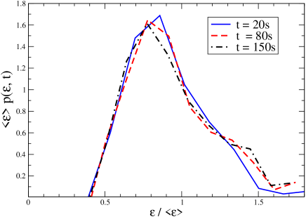
Figure 12: Scaling functions of strain fields $f(\epsilon/\langle\epsilon\rangle;t)$ from experiments on paper using $l=14$ mm, crate 16x16 and SSD 0.05 pixels. Different lines indicate the time at which $f$ is computed, chosen to be at the beginning, in the middle and at the end of primary creep. The average distribution over 16 different samples is computed by taking all the local displacements at a given time and then computing the scaling function from the distribution $p(\epsilon;t)$. The scaling functions collapse and are consistent with the scaling hypothesis of an absorbing state phase transition (Equation (12)). The distributions have a similar asymmetric form and a large-strain tail which is decaying in an exponential fashion.

In Figure 12 we depict the scaling functions $f(\epsilon/\langle\epsilon\rangle;t)=\langle\epsilon\rangle p(\epsilon;t)$ during the primary creep in experiments on paper. The deformation data $\epsilon(t)$ is averaged over 16 samples. Similar result for the scaling of the distribution are obtained for the DDD simulations as is shown in Figure 13. The variance $\Delta\epsilon^{2}(t)$ is shown in Figures 14 and 15. During the primary Andrade creep the variance of the fluctuations increases as $\Delta\epsilon^{2}\sim t^{0.75}$ in the paper experiments and close to $t^{2/3}$ in the DDD simulations. The results indicate that the scaling hypothesis is plausible. The slightly larger exponent observed in the case of the paper experiment could be related to the experiments being somewhat subcritical. One can also extend the experimental data beyond the range in time appropriate for Andrade creep, with at least a rough agreement with the expected behaviour for the logarithmic creep phase (an exponent larger than the $0.75$ for the Andrade regime is found). Notice that the result that the spatial fluctuations of the integrated strain exhibit the same scaling as their mean is not in contradiction with the observation that the fluctuations of the strain rate scale differently from their mean.

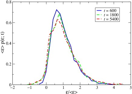
Figure 13: Scaling functions $f(\epsilon/\langle\epsilon\rangle,t)$ from discrete dislocation simulations. Distributions of the integrated local strain for three different times for the critical stress value $\sigma_{c}\approx 0.025$, scaled according to Equation (12). The box size used is $l=25b$. For larger $l$ (not shown) the scaling function becomes more narrow, possibly approaching the shape of the experimental distributions (Figure 12) for large $l$. The both tails of the distributions can be well described by an exponential.

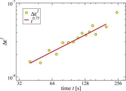
Figure 14: Variance of the probability distribution of the total deformation $p(\epsilon;t)$ as a function of time from experiments on paper. The result is the averaged variance over 16 experiments. The scaling behaviour corresponds to the Andrade’s scaling of the experimental data where $\epsilon_{t}\sim t^{-0.7...0.8}$. This behaviour is in agreement with the scaling behaviour shown in the previous figure.

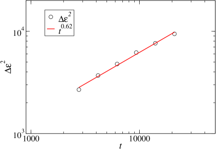
Figure 15: Variance of the probability distribution of the total deformation as a function of simulation time from dislocation simulations, at $\sigma\approx\sigma_{c}$. The data corresponds to that in Figure 13. The line indicates a scaling derived from an Andrade law. A least-squares fit to the data gives a slightly smaller exponent (0.62). The data is averaged over 16 samples.

Finally we analyze the spatial correlation functions of the integrated order parameter or the creep strain field. Given that the experimental strain fields are two-dimensional, we can study the correlations in two independent directions. The horizontal correlation function is defined as the width

$$w_{x}(r,t)=\sqrt{\langle(\epsilon(x+r,y_{c})-\epsilon(x,y_{c}))^{2}\rangle_{x}},$$ (16)

where the roughness of the $y$-directional strain $\epsilon$ is averaged over the $x$-coordinate in a constant position $y_{c}$. Thus this represents the 1-dimensional correlations of the integrated strain for a fixed height $y_{c}$ which we choose to study here for simplicity, given that it is difficult to fix a reference coordinate system on the sample surface. Analogously, the vertical correlation function is defined as

$$w_{y}(r,t)=\sqrt{\langle(\epsilon(y+r,x_{c})-\epsilon(y,x_{c}))^{2}\rangle_{y}}.$$ (17)

The scaling behaviour of the width $w(r,t)$ (both $w_{x}$ and $w_{y}$) is expected to be governed by the scaling form

$$w(r,t)=t^{1-\theta}f\left(\frac{t}{r^{z}}\right),$$ (18)

where the above “simple” scaling picture has been assumed to hold, such that $\beta=1-\theta$. In Figure 16 we show the squared deformation-deformation correlation functions $w_{x}^{2}(r,t)$ and $w_{y}^{2}(r,t)$ for three different correlation distances $r$ from a typical experiment. For the horizontal direction we observe scaling with an exponent $2-2\theta$ close to 2/3, i.e. consistent with the simple scaling picture and the usual scaling exponent of the Andrade’s law, $\theta\approx 2/3$. In the vertical direction the statistics is not so good, and it is not possible to conclude if the system exhibits anisotropic scaling or not. The overall relatively poor statistics also made it impossible to test in detail the possible $r$-dependent saturation as implied by Equation (18).

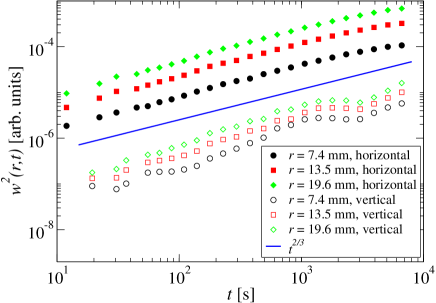
Figure 16: An example of the squared deformation-deformation correlation functions $w(r,t)^{2}$ (Equation (18)) from a single experiment with $t_{c}~{}=~{}6324$s, $l=12.3$ mm, in horizontal ($w_{x}^{2}(r,t)$, filled symbols) and vertical ($w_{y}^{2}(r,t)$, open symbols) directions. The solid line corresponds to the $t^{2/3}$ behavior, as derived from the Andrade’s law. The statistics of the data is insufficient in order to conclude the form of the scaling function $f(r,t)$ in Equation (18). Also attempts to check for the possibility of anisotropic scaling failed due to poor statistic in the vertical data.

3.7 Spatial order parameter fluctuations at the depinning transition

For the sake of comparison, we finish by considering the spatial order parameter (=velocity) fluctuations exhibited by driven interfaces close to the depinning threshold. To this end, we choose to study the $d=2+1$ Linear Interface Model (LIM), or quenched Edwards-Wilkinson (qEW) equation,

$$\frac{\partial h(x,y,t)}{\partial t}=\nu\nabla^{2}h(x,y,t)+\eta(x,y,h)+F,$$ (19)

where $h(x,y,t)$ is the local interface height at time $t$, $\nu$ is the surface tension, $\eta(x,y,t)$ is a quenched random force term with correlations $\langle\eta(x,y,h)\eta(x^{\prime},y^{\prime},h^{\prime})\rangle=2D\delta(x-x^{\prime})\delta(y-y^{\prime})\delta(h-h^{\prime})$, and $F$ is the external force. We simulate the model in continuous time, for linear system sizes up to $L=256$.

The top panel of Figure 17 shows the spatially averaged interface velocity $\langle v\rangle$, and the spatial fluctuations of the local interface velocities $\delta v$ for $l=2$ and $\Delta t=1$ as a function of time $t$ for different values of the external force $F$. Close to a critical value $F=F_{c}$, both quantities follow asymptotically a power law in time, the average velocity obeying $\langle v\rangle\sim t^{-\theta}$, with $\theta\approx 0.51$. This is in good agreement with earlier results, assuming a scaling relation $\theta=1-\beta$, where $\beta\approx 0.48$ is the growth exponent [39]. The fluctuations follow $\Delta v\sim t^{-\gamma}$, with $\gamma\approx 0.25$. For $F>F_{c}$ and $F<F_{c}$, both the mean and the fluctuations deviate from the power law, approaching a finite constant value for $F>F_{c}$, and decaying exponentially to zero for $F<F_{c}$.

Considering different length scales $l$ and system sizes $L$ reveals that the growth of correlations plays a central role in the scaling of the fluctuations. The characteristic power law at $F=F_{c}$ is observed only after a transient with an $l$ dependent duration. The relative fluctuations $\Delta v/\langle v\rangle$ at $F=F_{c}$ for different $l$ can be collapsed according to the scaling form

$$\Delta v/\langle v\rangle=l^{z(\theta-\gamma)-\delta}f(t/l^{z}),$$ (20)

involving the dynamic exponent $z\approx 1.56$ [39], and an exponent $\delta$ characterizing the $l$ dependence of the fluctuation amplitude. The main figure in the middle panel of Figure 17 shows a data collapse with $z=1.56$, $\theta-\gamma=0.26$ ($\approx\theta/2$), and $\delta=0.55$. This collapse suggests that the initial transient is related to the time $t^{*}\sim l^{z}$ it takes for the correlation length $\xi$ to reach the observation scale $l$. On the other hand, the duration of this power law is also limited by the finite system size: The late time data for $l=2$ and $\Delta t=1$ collapsed according to

$$\Delta v/\langle v\rangle=L^{z(\theta-\gamma)}g(t/L^{z})$$ (21)

and shown in the inset of the middle panel of Figure 17 shows that the power law describing the relative fluctuations $\Delta v/\langle v\rangle$ extends only up to a time $t^{**}\sim L^{z}$.

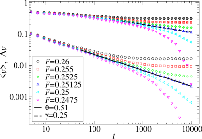
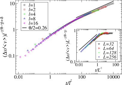
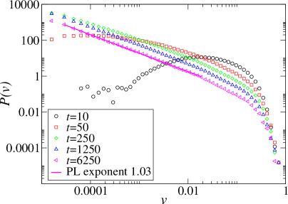
Figure 17: Average and standard deviation of the interface velocity in the $d=2+1$ LIM/qEW. Top: Average (open symbols) and standard deviation (filled symbols) of the local interface velocities for different external forces $F$ in the proximity of the critical force $F_{c}\approx 0.25125$, for $l=2$ and $\Delta t=1$. At the critical point, both exhibit a power-law decay in time, with exponents $\theta=0.51$ and $\gamma=0.25$, respectively. The fluctuation data has been displaced vertically for clarity. Middle: Scaling of the relative interface velocity fluctuations for $F=F_{c}$ for different $l$ (main figure). The inset shows the late time scaling for different system sizes $L$. In both cases the data can be collapsed with the dynamical exponent $z=1.56$. Bottom: The distributions of the local interface velocities for different times, for $F=F_{c}$, $l=2$ and $\Delta t=1$. The decreasing amplitude in the long time limit implies that an increasing fraction of the interface is no longer moving.

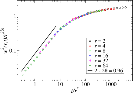
Figure 18: Scaling of the squared correlation functions $w^{2}(r,t)$ in the $d=2+1$ LIM/qEW in the long time limit, for different correlation distances $r$. The solid line corresponds to $2\beta=2-2\theta=0.96$, and $z=1.56$ controls the $r$-dependent saturation.

To understand the origin of the fluctuation exponent $\gamma$ in this case, it is useful to consider the distribution of the local velocities (from which $\delta v$ is obtained as the standard deviation) as a function of time. The bottom panel of Figure 17 shows that the distribution evolves with time from a peaked one towards a power law with a cutoff. By normalizing the distributions by the total number of data points (including the ones indistinguishable from zero) reveals that the amplitude of the power law decreases with time, but otherwise the distribution remains unchanged: Notice in particular how the large-velocity cut-off of the distribution is independent of time. Thus, the velocity distribution, after the initial transient, can be well described by the superposition

$$P(v^{i,j})=pP_{m}(v^{i,j})+(1-p)\delta(v^{i,j}),$$ (22)

where $P_{m}$ is the distribution of the mobile interface elements, which is found to be independent of time after a transient. The full distribution then evolves only via the decay of $p$, describing the fraction of observation boxes with a finite velocity. Thus, in the case of the LIM/qEW, an argument similar to the simple box argument, Equation (11), leads to a fluctuation exponent $\gamma=\theta/2\approx 0.26$, in good agreement with the numerical estimate $\gamma\approx 0.25$.

Finally we also consider the (isotropic) height-height correlations

$$w(r,t)=\sqrt{\langle(h(\vec{r}_{0}+\vec{r},t)-h(\vec{r}_{0},t))^{2}\rangle_{\vec{r}_{0}}},$$ (23)

analogously to Equations (16) and (17). After an initial transient, these obey the expected scaling form, Equation (18), with the scaling function shown in Figure 18. The early time growth of the roughness scales with the expected exponent $2\beta=2-2\theta=0.96$, followed by an $r$-dependent saturation, controlled by the dynamical exponent $z=1.56$.

The implications of these results for the creep deformation studies are as follows: As the fluctuation exponent $\gamma$ appears to be larger than $\theta/2$ in the case of paper experiments and the DDD simulations, the box argument, Equation (11), would imply that also the strain rate distribution of the active elements of the system would evolve in time, to yield the observed scaling of the fluctuations. Detailed analysis of this kind is however difficult as it would require a substantial amount of statistics, and is thus out of scope of the present study. Analysis involving growing correlations (in the spirit of Equations (20) and (21)) could also be complicated by the possibly anisotropic nature of such correlations [6].

4 Conclusions

The creep deformation of solids shows, after all, fluctuation features that are unexpected. Clearly it is to be expected that in any not completely homogenenous and translationally invariant material (sample) the rheology has to include in practice a fluctuating component. However, the spatiotemporal aspects that it then encompasses first of all are not included in traditional materials science descriptions of empirical data, and secondly they may - as indeed is the case here - originate from “collective behavior”. And, this is the central point of the current investigation.

The presence of crackling noise in materials is of course an old subject, from Barkhausen noise in magnets to acoustic emission in the brittle fracture -related deformation of materials and geosystems. In these two particular cases, theory has been able to explain to a varying degree from almost complete to qualitative the features seen such as probability distributions of noise events, and correlations in the timeseries measured. An open problem here, and in many other similar systems where one can study collective phenomena in deformation - such that possess a jamming transition for instance - either experimentally or numerically or both, is what is the coarse-grained theory like, and what is the origin of the eventual criticality and the general picture of the fluctuations that ensue. In dislocation plasticity, various attempts of the scaling argument -type have been done to understand creep in addition to numerical models from DDD to cellular automata. However, no formulation exists that would account for the yielding transition faithfully. Obviously, in non-crystalline materials the search is even further away from a candidate in spite of various rheology-based attempts that have been done lately. Thus we conclude that experiments such as published here, including the numerical ones, should also offer a valuable guideline for future developments.

In addition to showing that scaling exists in the fluctuations in primary (Andrade) and logarithmic creep, we have also shown the results of the application of various ideas from absorbing phase transitions, including depinning transitions for elastic manifolds in random media. It appears that the part of creep that would originate from a yielding transition agrees with this picture. Our experiments nevertheless suffer from a lack of resolution in space and time, and it is to be hoped that a better (two-dimensional) test material is found to improve on both. This is true for the creep rate correlation functions. We note also that the presence of fluctuations in the logarithmic phase is not a priori easy to relate to a phase transition picture unlike for the preceding Andrade part. The same goes also for the untested behavior in tertiary creep as the sample failure is approached.

Creep is the simplest paradigm of time-dependent failure. What we describe here is the development of creep strain mostly when there is not yet actually any damage, i.e. in the classical empirical creep language the system is not yet in tertiary creep. This overview raises a wide variety of open questions. First, what happens in a ordinary tensile test with a certain strain rate, what is the role of the viscoplastic deformation in a (apparently) brittle material say, or in a very ductile one if one assumes that similar collective phenomena are to be found there as well? An analogy from depinning is a ramp of the driving force so that eventually the threshold is crossed. Second, the role of temperature in depinning (and in DDD models) has a specific meaning. It influences i) the mobility of the coarse-grained dynamics (scales the timescale in DDD) and ii) it leads to ”creep” or thermally assisted motion or deformation at the end - but beyond the criticality-dependent creep. Third, what is the role of such phenomena in materials science, if any? Fourth, one can now go beyond creep to various scenarios of time-dependent material failure such as fatigue etc., and repeat the experiments and the analysis in such cases. One question is the role of relaxation processes or memory effects: how will these influence strain rate fluctuations, and if as for elastic manifolds one finds signatures of the behavior of glassy systems. An example of such could be aging, for which many separate scenarios could be envisioned.

In summary, we have discussed in this article by experiments on a two-dimensional material (i.e. paper) and by simulating a crystal plasticity model, that creep deformation shows fluctuations that can be analyzed further using the language of absorbing state phase transitions. For DDD models the existence of the yielding transition has been known, and it has been recently established to be a peculiar, zero-temperature second-order phase transition. The observations we have made are of course related to the critical scaling thereof: how exactly is still to be understood. The experimental signatures from a non-crystalline material are quite similar, which would hint of a greater universality than what one might have expected. Future work should include settling some of the open issues listed above, and we would also like to underline the possibilities in other systems including model ones such as colloidal particle assemblies, with both crystalline order and in the amorphous state [40, 41].

References

References

- [1] Andrade E N da C 1910 Proc. R. Soc. A 84 1
- [2] Rosti J, Koivisto J, Laurson L and Alava M J 2010 Phys. Rev. Lett. 105 100601
- [3] Louchet F and Duval P 2009 Int. J. Mat. Res. 100 1433
- [4] Miguel M C, Vespignani A, Zaiser M and Zapperi S 2002 Phys. Rev. Lett. 89 165501
- [5] Zaiser M and Moretti P 2005 J. Stat. Mech. P08004
- [6] Laurson L, Miguel M C and Alava M J 2010 Phys. Rev. Lett. 105 015501
- [7] Miguel M C, Vespignani A, Zapperi S, Weiss J and Grasso J R 2001 Nature 410 667
- [8] Weiss J and Marsan D 2003 Science 299 89
- [9] Dimiduk D M, Woodward C, LeSar R and Uchic M D 2006 Science 312 1188
- [10] Jakobsen B, Poulsen H F, Lienert U, Almer J, Shastri S D, Sørensen H O, Gundlach C and Pantleon W 2006 Science 312 889
- [11] Zaiser M, Grasset F M, Koutsos V and Aifantis E C 2004 Phys. Rev. Lett. 93 195507
- [12] Csikor F F, Motz C, Weygand D, Zaiser M and Zapperi S 2007 Science 318 251
- [13] Nabarro F R N and Villiers F De 1995 Physics of Creep and Creep-Resistant Alloys (London: Taylor & Francis)
- [14] Barrat J L and Lemaitre A 2011 Dynamical heterogeneities in glasses, colloids, and granular media ed L Berthier, G Biroli, J-P Bouchaud, L Cipelletti and W van Saarloos (Oxford University Press)
- [15] Maloney C and Lemaitre A 2004 Phys. Rev. Lett. 93 016001
- [16] Goyon J, Colin A, Ovarlez G, Ajdari A and Bocquet L 2008 Nature 454 84
- [17] Dauchot O, Durian D and van Hecke M 2011 Dynamical heterogeneities in glasses, colloids, and granular media ed L Berthier, G Biroli, J-P Bouchaud, L Cipelletti and W van Saarloos (Oxford University Press)
- [18] Liu A J and Nagel S R 1998 Nature 396 21
- [19] Keys A S, Abate A R, Glotzer S C and Durian D J 2007 Nature Phys. 3 260
- [20] Berthier L, Biroli G, Bouchaud J P and Jack R 2011 Dynamical heterogeneities in glasses, colloids, and granular media ed L Berthier, G Biroli, J-P Bouchaud, L Cipelletti and W van Saarloos (Oxford University Press)
- [21] Groma I 1997 Phys. Rev. B 56 5807
- [22] Coffin D W 2005 Advances in Paper Sci. and Tech. ed S J I’Anson (Lancashire: FRC), p 651
- [23] Van der Giessen E and Needleman A 1995 Model. Simul. Mater. Sci. Eng. 3 689
- [24] Csikor F F, Zaiser M, Ispanovity P D and Groma I 2009 J. Stat. Mech. P03036
- [25] Salminen L I, Pulakka J M, Rosti J, Alava M J and Niskanen K J 2006 Europhys. Lett. 73 55
- [26] Kybic J and Unser M 2003 IEEE Trans. Image Process. 12 1427
- [27] Hild F and Roux S 2006 Strain 42 69
- [28] Sutton M A, Turner J L, Bruck H A and Chae T A 1991 Exp. Mech. 31, 168
- [29] Kybic J, Thevenaz P, Nirkko A and Unser M 2000 IEEE Trans. Med. Imaging 19 80
- [30] Mustalahti M, Rosti J, Koivisto J and Alava M J 2010 J. Stat. Mech. P07019
- [31] Talamali M, Petäjä V, Vandembroucq D and Roux S 2008 Phys. Rev. E 78 016109
- [32] Nechad H, Helmstetter A, El Guerjouma R and Sornette D 2005 Phys. Rev. Lett. 94 045501
- [33] Monkman F C and Grant M 1956 Proc ASTM 56 593
- [34] Cottrell A H 2004 Phil. Mag. Lett. 84 685
- [35] Mott N F 1953 Proc. R. Soc. Lond. A 220 1
- [36] Miguel M C, Laurson L and Alava M J 2008 Eur. Phys. J B 64 443
- [37] Alava M J and K J Niskanen 2006 Rep. Prog. Phys. 69 669
- [38] Dickman R and Muñoz 2000 Phys. Rev. E 62 7632
- [39] Leschorn H, Nattermann T, Stepanow S and Tang L H 1997 Ann. der Physik 509 1
- [40] Pertsinidis A and Ling X S 2005 New J. Phys. 7 33
- [41] Schall P, Weitz D A and Spaepen F 2007 Science 318 1895