pacce: Perl Algorithm to Compute Continuum and Equivalent Widths

Abstract

We present Perl Algorithm to Compute continuum and Equivalent Widths (pacce). We describe the methods used in the computations and the requirements for its usage. We compare the measurements made with pacce   and “manual” ones made using iraf splot task. These tests show that for SSP models the equivalent widths strengths are very similar (differences $\lesssim$ 0.2 Å) for both measurements. In real stellar spectra, the correlation between both values is still very good, but with differences of up to 0.5 Å. pacce  is also able to determine mean continuum and continuum at line center values, which are helpful in stellar population studies. In addition, it is also able to compute the uncertainties in the equivalent widths using photon statistics. The code is made available for the community through the web at http://www.if.ufrgs.br/$\sim$riffel/software.html.

Not to appear in Nonlearned J., 45.

Keywords Methods: data analysis; Line: Equivalent Widths; Techniques: Spectroscopy

1 Introduction

The equivalent widths ($W_{\lambda}$) of absorption lines, observed in the spectrum of astronomical sources can be seen as compressed, but highly informative, representation of the whole spectrum. For example, the $W_{\lambda}$ of the absorption lines observed in galaxies spectra reveals insights about their stellar populations, like the ages and metallicities of the stars which dominates the light of the host galaxy (e.g. Bica, 1988; Schmitt et al., 1996; Rickes et al., 2004; Rembold & Pastoriza, 2007; Krabbe et al., 2007, 2008; Riffel et al., 2008). Regarding the spectrum of a star, it is possible to make use of the $W_{\lambda}$ of absorption lines to determine directly the fundamental atmospheric parameters such as: surface gravity ($\log g$), effective temperature ($T_{\rm eff}$) and the chemical abundances of many elements (see for example Gonzalez & Lambert, 1996; Feltzing & Gonzalez, 2001).

However, the price to be paid when using the powerful informations contained in the $W_{\lambda}$ is the long time needed to make a reliable measurement of this observables. Commonly, the $W_{\lambda}$ are measured using interactive routines like splot provided by the IRAF team or with independent codes like LINER (Pogge & Owen, 1993). Both softwares are “hand operated”, which means the user need to look for the line limits and continuum points in the spectrum. The next step, is to mark them “manually”. This procedure is very time-consuming and introduce many uncertainties which are propagated to a posterior analyses of the quantities involving the $W_{\lambda}$ measurements.

With the growing of spectral surveys (e.g. Sloan Digital Sky Survey), it becomes necessary to accelerate and automate some process such as the analysis of stellar populations of galaxies, as well as the determination of fundamental atmospheric parameters of individual stars. In order to help in such task we present in this paper a new automatic code: PACCE: Perl Algorithm to Compute Continuum and Equivalent Widths. This software, written in PERL, can be used to compute the $W_{\lambda}$ of absorption lines as well as to determine continuum points, being very helpful to perform stellar population synthesis following, for example the method developed by Bica (1988) and Schmitt et al. (1996).

This paper is structured as follows: In Sec. 2 we describe the system requirements as well as the numerical procedures behind the code. The input parameters and the outputs of the code are discussed in Sec. 3. A comparison with the measures made whit pacce  and “hand-made” measurements are presented in Sec. 4. The final remarks are made in Sec. 5.

2 The code

The idea behind pacce is to reproduce the “manual” procedure used to measure the $W_{\lambda}$ of absorption lines in a spectrum, as well as to measure mean continuum fluxes in defined regions and compute the continuum value at line center. In addition, using the same inputs, it does exactly reproduce the measured values being “user” independent (e.g. the uncertainties introduced by the user in “hand operated” procedures are removed), and thus allowing for a better comparison between $W_{\lambda}$ measured by different users.

pacce was written in Perl, allowing anyone to use it without having any problems with software licenses. It is freely distributed under GNU General Public License(GLP). All the libraries used in the code are also free and distributed under GLP license. pacce  source code can be freely downloaded from http://www.if.ufrgs.br/$\sim$riffel/software.html. All requirements to run pacce can easily be installed in any linux machine (e.g. apt-get, synaptic or yum), they are:

• Perl
  (http://www.perl.org);

• Perl’s ”Math::Derivative” package
  (http://search.cpan.org);

• Perl’s ”Math::Spline” package
  (http://search.cpan.org);

• Gnuplot
  (www.gnuplot.info).

In addition, we call the attention to the fact that Perl is installed as default in any linux flavor and pacce  can easily be converted to run under Microsoft Windows system (without plots).

Fig. 1 : Fluxogram describing the use of pacce .

2.1 Calculations: Equivalent Widths and Mean Continuum Fluxes

2.1.1 Equivalent Widths

In general, absorption feature indices are composed by measurements of relative flux in a central wavelength interval corresponding to the absorption feature considered (line limits $\lambda_{l}$ and $\lambda_{u}$ in Fig.  2) and two continuum sidebands passband regions (spectrum ranges - dots - in the boxes of Fig.  2). Such sidebands provide a reference level (pseudo-continuum, solid line Fig.  2) from which the strength of the absorption feature is evaluated (see Worthey et al., 1994, for details). pacce computes the pseudo-continuum, $F_{c}(\lambda)$, in three ways: (i) a linear regression is computed using all the continuum points in the passband regions and a straight line (y=ax+b) is computed using the regression coefficients; (ii) a straight line is drawn connecting the mid-points of the flanking passband continuum regions; (iii) as a cubic spline. The form in which the pseudo-continuum is adjusted is chosen by the user (see Sec. 3).

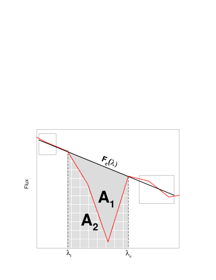
Fig. 2 : Sketch of the definition of a hypothetical index. Sidebands continuum regions are represented by boxes. Solid line is the pseudo-continuum. Vertical lines represent the line limits $\lambda_{l}$ and $\lambda_{u}$. Shaded region (A₂) is the area below the line limits and filled (A₁) region is the area of the line. Dotted line (red) represents the spectrum.

Considering $F_{i}(\lambda)$ as observed flux per unit wavelength an $W_{\lambda}$ is then:

$$\centering W_{\lambda}=\displaystyle\int_{\lambda_{l}}^{\lambda_{u}}\left(1-\frac{F_{i}(\lambda)}{F_{c}(\lambda)}\right)d\lambda\@add@centering$$ (1)

Considering Fig.  2 one can write the area A₂ as:

$$A{\rm{}_{2}=}\displaystyle\int_{\lambda_{l}}^{\lambda_{u}}F_{i}(\lambda)d\lambda$$ (2)

and, thus, the A₁ is the absorbed flux between $\lambda_{l}$ and $\lambda_{u}$. Similarly, the area below the pseudo-continuum between $\lambda_{l}$ and $\lambda_{u}$ is:

$$A{\rm{}_{1}}+A{\rm{}_{2}=C=}\displaystyle\int_{\lambda_{l}}^{\lambda_{u}}F_{c}(\lambda)d\lambda,$$ (3)

thus, the $W_{\lambda}$ of the absorption line between $\lambda_{l}$ and $\lambda_{u}$ can be written as:

$$W_{\lambda}=\displaystyle\left(1-\frac{A_{2}}{C}\right)(\lambda_{u}-\lambda_{l}),$$ (4)

for more details see for example Vollmann, & Eversberg (2006).

In pacce  we compute both areas, A₂ and C, using the trapezium method. In addition, pacce  does compute the uncertainties in the equivalent widths, $\sigma(W_{\lambda}$), considering the photon noise statistics pixel by pixel. For this purpose we follow Vollmann, & Eversberg (2006), assuming that the ratio between C and A₂ are similar to the normalized ratio between these quantities (for details see Vollmann, & Eversberg, 2006). In the case of linear pseudo-continuum adjustment we estimate the signal-to-noise ratio (S/N) as being the ratio between the square root of the variance and the mean flux of the points in the bandpass interval (i.e. boxes in Fig  2). In the case of a pseudo-continuum defined with a cubic spline the S/N is calculate in the same way as in the linear adjustment, but using points in a region free from emission/absorption lines defined by the user (see Sec. 3).

2.1.2 Mean Continuum Fluxes

Besides the $W_{\lambda}$  the code also computes the mean continuum fluxes ($\bar{F_{\lambda}}$, last line of Tab. 1) and the continuum at line center. Such measurements are useful, for example, to perform stellar population studies using the technique described by Bica (1988). The $\bar{F_{\lambda}}$ point are calculated following the equation:

$$\bar{F_{\lambda}}=\displaystyle\frac{1}{N}\sum_{i=0}^{i=N}F_{\lambda}^{i},$$ (5)

where $F_{\lambda}^{i}$ is the flux of each $\lambda$ in the defined interval and N is the number of points considered. The errors are estimated as being the square root of the variance. The continuum at the line center is taken as being the pseudo-continuum flux where $\lambda=\frac{\lambda_{l}+\lambda_{u}}{2}$.

3 Running pacce

To run pacce the user needs a ASCII, one dimensional, spectrum and a ASCII input table containing the line definitions. The ASCII spectrum is easily created using the wspectext iraf task. An example of a input table is shown in Tab. 1. Note that the continuum points used to determine the line pseudo-continuum can be defined into three different ways (linear, mid-point or spline). The fact that such input table is very easy to be edited/created, makes pacce  also an interactive tool, allowing for fast changes and tests in $W_{\lambda}$ and $\bar{F_{\lambda}}$ measurements.

Besides the calculations, pacce  outputs some auxiliary files (Fig.  1). These files are the pseudo-continuum data points, the plots showing the regions used in the $W_{\lambda}$ calculations (see Fig.  3), as well as the Gnuplot commands, which are stored for future use.

    #####################################################################################
    #                                                                                   #
    #                   Index definitions table example.                                #
    #                                                                                   #
    #####################################################################################
    #  ID             Line Limits          Left side Cont.     Right side Cont.
       LinearC       (4847.875,4876.625)  [4827.875:4847.875],[4876.625:4891.625]
       MidPntC       (4847.875,4876.625)  [4827.875:4847.875],[4876.625:4891.625]*
    # Note the * in the mid-point continuum adjustment.
    ######################### Spline continuum example ##################################
    #  ID         Line Band Pass       Points for a Spline Cont.              S/N cont.
    spline    (4847.875,4876.625) {4827.875,4833.0,4847.875,4876.625,4891.625}<4880:4890>
    #####################################################################################
    #                                                                                   #
    #                         Intervals for Mean continuum                              #
    #                         see Bica (1986)                                           #
    #####################################################################################
    #
    Cont. |5290:5310,5303:5323,5536:5556,5790:5810,5812:5832,5860:5880,6620:6640|

Table 1 : Example of input table. A # indicates that the line is not used in the computations. Note the $*$ in the mid-point continuum adjustment. A full table is available at http://www.if.ufrgs.br/$\sim$riffel/software.html.

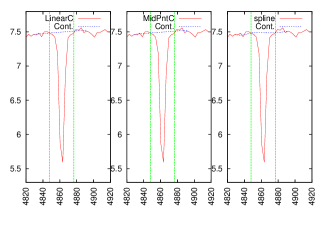
Fig. 3 : Example of pacce  output plots using Tab. 1 index definitions. Mid-point, linear and spline pseudo-continuum adjustments where used in left, center and right plots respectively. The shown region is around H$\beta$ absorption line.

4 Testing pacce

In order to test pacce  we perform “hand-made” measurements in a set of Maraston (2005) simple stellar population (SSP) models as well as in a library of observed stellar optical spectra (Silva & Cornell, 1992).

In Fig.  4 we show a comparison $\sim$3600 $W_{\lambda}$ measured using pacce  and ‘ ‘hand-made” measurements with iraf splot task. We also plot the differences between the measurements and make a histogram of these differences to give a better idea of the dispersion between both sets. It is clear from Fig.  4 that pacce  does reproduce very well the splot “manual” $W_{\lambda}$ values. Note that there seems to be a very slight systematic under-prediction of the $W_{\lambda}$ computed with pacce  if compared with those of splot, however, the differences are $\lesssim$0.05Å. Similar results were obtained by Sousa et al. (2007, see their Fig. 6), thus, suggesting that iraf splot measurements may slightly overestimate the $W_{\lambda}$ values.

Fig. 4 : Comparation of pacce  and “hand made” iraf splot measurements using Maraston (2005) theoretical models. Solid line is the equivalence line. At the differences and a histogram of them are shown in bottom and right side, respectively.

It is even harder to properly measure $W_{\lambda}$ in observed spectra than in theoretical ones. To properly test our code capability in dealing with real spectra we have measured a set of $W_{\lambda}$  ($\sim$ 950$W_{\lambda}$) in the library of observed stellar spectra presented by Silva & Cornell (1992). The results of such test are shown in Fig.  5. It is clear that pacce  is able to properly reproduce the measurements of splot task. However, a larger dispersion in the differences is observed between both measurements than when using SSP models. In addition, these differences are clearly within the errors and are lower than $\sim$0.5Å.

Fig. 5 : Same as Fig.  4 but for observed optical stellar spectra. Error bars are shown.

5 Final Remarks

We present pacce  a Perl algorithm to compute continuum and $W_{\lambda}$. We describe the method used in the computations, as well as the requirements for its use.

We compare the measurements made with pacce   and “manual” ones made using iraf splot task. These tests show that for SSP models (i.e. high S/N) the $W_{\lambda}$ values are very similar (differences $\lesssim$ 0.2 Å). In real stellar spectra, the correlation between both values is also very good, but with differences of up to 0.5 Å. However, these small differences can be explained by the intrinsic errors in subjectiveness determinations of continuum levels caused in “manual” measurements.

pacce  is also able to determine mean continuum and continuum at line center values, which are helpful in stellar population studies. In addition, it is also able to compute the $\sigma(W_{\lambda})$ using photon statistics.

References

- Bica (1988) Bica, E. 1988, A & A, 195, 76.
- Feltzing & Gonzalez (2001) Feltzing, S. & Gonzalez, G., 2001, A&A, 367, 253.
- Gonzalez & Lambert (1996) Gonzalez, G. & Lambert, D. L. 1996, AJ, 111, 424.
- Krabbe et al. (2007) Krabbe, A. C., Rembold, S. B. & Pastoriza, M. G., 2007, 2007, MNRAS, 378, 569.
- Krabbe et al. (2008) Krabbe, A. C.; Pastoriza, M. G.; Winge, C.; Rodrigues, I.; Ferreiro, D. L., 2008, MNRAS, 389, 1593.
- Maraston (2005) Maraston, C., 2005, MNRAS, 362, 799.
- Pogge & Owen (1993) Pogge, R. W., & Owen, J. M. 1993, OSU Internal Report 93-01
- Rembold & Pastoriza (2007) Rembold, S. B. & Pastoriza, M. G., 2007, MNRAS, 374, 1056
- Rickes et al. (2004) Rickes, M. G., Pastoriza, M. G. & Bonatto, Ch., 2004, A&A, 419, 449
- Riffel et al. (2008) Riffel, R.; Pastoriza, M. G.; Rodríguez-Ardila, A. & Maraston, C., 2008, MNRAS, 388, 803.
- Schmitt et al. (1996) Schmitt, H. R., Bica, E., & Pastoriza, M. G. 1996, MNRAS, 278, 965
- Silva & Cornell (1992) Silva, D. R.; Cornell, M. E., 1992, ApJS, 81, 865.
- Sousa et al. (2007) Sousa, S. G., Santos, N. C., Israelian, G., Mayor, M. & Monteiro, M. J. P. F. G., 2007, A&A, 469, 783.
- Vollmann, & Eversberg (2006) Vollmann, K. & Eversberg, T., 2006, AN, 327, 862.
- Worthey et al. (1994) Worthey, G.; Faber, S. M.; Gonzalez, J. J. & Burstein, D., 1994, ApJS, 94, 687.