Exchange interactions and magnetic phases of transition metal oxides: benchmarking advanced ab initio methods.

Abstract

The magnetic properties of the transition metal monoxides MnO and NiO are investigated at equilibrium and under pressure via several advanced first-principles methods coupled with Heisenberg Hamiltonian MonteCarlo. The comparative first-principles analysis involves two promising beyond-local density functionals approaches, namely the hybrid density functional theory and the recently developed variational pseudo-self-interaction correction method, implemented with both plane-wave and atomic-orbital basis sets. The advanced functionals deliver a very satisfying rendition, curing the main drawbacks of the local functionals and improving over many other previous theoretical predictions. Furthermore, and most importantly, they convincingly demonstrate a degree of internal consistency, despite differences emerging due to methodological details (e.g. plane waves vs. atomic orbitals).

I Introduction

The relative simplicity of structural and magnetic ordering and the abundance of available experimental and theoretical data elect transition metal monoxides (TMO) as favorite prototype materials for the ab initio study of exchange interactions in Mott-like insulating oxides.anderson59 TMO are known to be robust antiferromagnetic (AF) Mott insulators with sizable exchange interactions and Néel ordering temperatures. The accurate determination of magnetic interactions purely by first-principles means is a remarkable and as yet unsolved challenge.solovyev ; wan ; kotani The difficulty stems, on the one hand, from fundamental issues in the description of Mott insulators by standard density functional theory (DFT) approaches, such as local-spin density approximation (LDA) or the generalized gradient approximation (GGA). On the other hand, the determination of low-energy spin excitations require a meV-scale accuracy; however, the error bar due to specific implementation and technical differences may easily be larger.

A large amount of theoretical work for TMO has amassed over the years. A number of studies were carried out in particular for MnO and NiO with a variety of advanced methods: the LDA+U,dudarev ; fang ; solovyev ; rohrbach ; pask01 GGA+U,zhang ; bayer07 the optimized effective potential (OEP),solovyev the quasiparticle Green function (GW) approach,kotani ; arya ; massidda several types of self-interaction corrected LDA (SIC-LDA), svane ; szotek ; kodde ; fischer ; dane ; huges Hartree-Fock,towler ; bredow ; franchini ; moreira and several types of hybrid functionals such as B3LYP,feng ; moreira PBE0,franchini ; tran ; chen , Fock-35moreira , and B3PW91.tran From a methodological viewpoint, Refs. kasinathan, , solovyev, , and fischer, are particularly relevant for our present purposes, because of the systematic comparison of diverse approaches to computing magnetic interactions. Other studiescohen ; mattila ; kunes focused in particular on pressure-induced high-to-low spin magnetic collapse observed at very high pressure ($\sim$150 GPa for MnO) and relevant to Earth-core geophysics. Here we will not, however, be concerned with the phenomenology of this specific phase transition.

The present work presents a detailed theoretical analysis of MnO and NiO magnetic properties on a wide range of lattice parameters (i.e. hydrostatic pressures) carried out by an array of both standard and advanced first-principles methods. In particular, our theoretical front-liners are two approaches proposed recently for the description of strongly-correlated systems: the Heyd, Scuseria and Ernzerhof (HSE) hybrid functional approach,hse and the recently developed variational pseudo self-interaction correction,vpsic implemented in two different methodological frameworks: plane-wave basis set plus ultrasoftuspp pseudopotentials (PSIC), and linear combination of atomic-orbital basis set (ASIC). To provide a baseline for their evaluation, we complement these methods by their local counterparts implemented in the same methodological setting, namely LDA in plane-waves and ultrasoft pseudopotentials (reference for PSIC), local-orbitals and norm-conserving pseudopotentials (reference for ASIC), and GGA in the Perdew-Becke-Ernzerhofpbe (PBE) version (reference for HSE). Performing the same set of calculations in parallel with different methods, as well as different implementations of the same method is instrumental to distinguish fundamental and methodological issues, and characterizes this work with respect to the many previous theoretical studies of TMO.

MnO and NiO in equilibrium conditions have a high-spin magnetic configuration and large ($\sim$ 3.5-4 eV) band gap. Magnetic moments and exchange interactions depend crucially on the details of structural and electronic properties. The latter are characterized by a complex interplay of distinct energy scales: the crystal field splitting, which in rocksalt symmetry separates the on-site 3d $e_{g}$ and $t_{2g}$ energies; the charge transfer energy between O $p$ and TM d states; the hopping energies between d-d and p-d states.zaanen Ref.solovyev, convincingly shows that an empirical single-particle potential suitably adjusted to reproduce the experimental values of the above mentioned energies can deliver highly accurate magnetic interactions (moments and spin-wave dispersion). However, obtaining a correct balance of all these contributions is difficult even for advanced density functional methods, not to mention standard LDA or GGA, which fails altogether (to different extents depending on the specific compound). A general analysis of these failures and difficulties of ab initio approaches is beyond the scope of this work; we mention that the thorough analysis carried out in Ref.solovyev, and nekrasov08, suggests that a single parameter, as adopted by the LDA+U, is not sufficient, while global multi-state energy corrections could serve this purpose. Both the advanced methods (HSE and PSIC/ASIC) adopted in this work, while quite different in spirit, act in terms of ”global” corrections to local density functional energy spectrum, i.e. no a priori assumption is made about which particular state or band is in need of modification or correction.

A large portion of the LDA/GGA failure in the description of correlated systems can be imputed to the presence of self-interaction (SI) – that is, the interaction of each single electron with the potential generated by itself. One consequence of SI is a severe, artificial upshift in energy of the on-site single-particle energies in the density-functional Kohn-Sham equations (compared e.g. to measured photoemission energies). Spatially localized states are naturally characterized by a large SI: these will include 3d states, but also (albeit to a lesser extent) 2p states, and of course localized interface, surface, and point-defect states. It is sometime argued that this error is immaterial because Kohn-Sham eigenvalues are not supposed to match single-particle energies, and density-functional theories are only valid for ground-state properties. However, highest-occupied and lowest-unoccupied electronic states are exceptions, since the former must be rigorously related to the first ionization energy and thus is a ground-state property while the latter may also be interpreted within generalized KS schemes [Phys Rev B 53, 3764, (1996)] as an approximate electron addition energy. As a consequence, the SI error may dramatically affect the predicted ground state properties, even turning the Kohn-Sham band structure from insulating to metallic (a frequent occurrence for Mott-like systems in LDA/GGA).

MnO and NiO are both affected by SI, although to different extents:ff-coll severely for MnO, dramatically for NiO. Under positive (i.e. compressive) pressure the problem will be amplified, as any small band gap which may exist at equilibrium will be further reduced up to complete closure, and magnetic moments may be disrupted. Thus, a reliable description of TMO under pressure necessarily requires approaches overcoming the SI problem. Both PSIC/ASIC and HSE, although from different starting points, work towards the suppression of SI. The former explicitly subtracts the SI (written in atomic-like form) from the LDA functional; the latter, in a more fundamental manner, inserts of a portion of true Fock exchange in place of the local exchange functional, whose incomplete cancellation with the diagonal Hartree counterpart is the source of SI in LDA/GGA functionals.becke Our results will show that, despite the different conceptual origin, the two approaches deliver a systematically consistent description of MnO and NiO, in fact with spectacular quantitative agreement in several instances.

The paper is organized as following: Section II describes briefly the methodologies employed; in Section III, the model used to calculated the exchange-interaction parameters is discussed. Section IV illustrates our results at equilibrium (IV.1) and under pressure (IV.2). In Sections IV.2.2 and IV.2.3 we discuss the exchange interactions and critical temperatures, respectively. Section V offers some concluding remarks.

II Methods

Our first-principles results are obtained by using three different codes: PWSICpwsic , SIESTAsiesta and VASPvasp . With the PWSIC code, which uses plane-waves basis set and ultrasoft pseudopotentials we carry out calculations within LDA (hereafter LDA-PW) and PSIC. The SIESTAsiesta package, implemented over a local (atomic) orbital basis set and norm-conserving pseudopotentials, was employed for LDA (LDA-LO below) and ASIC calculations (note that the ASIC is available only in a developer version of the code). The variational PSIC/ASICvpsic approach evolves from the non-variational precursors PSICfs ; ff-coll and ASIC.asic The new method describes electronic properties as accurately as its precursors, and variationality allows its application to structural optimization and frozen-phonon calculations via quantum forces. In the following we briefly sketches the main features of the method, remanding the reader to Ref. [vpsic, ] for the detailed formulation for both plane waves (PSIC) and local orbital (ASIC) basis set.

The PSIC starts from the following energy functional

$$E^{PSIC}[\{\psi\}]\,=\,E^{LDA}[\{\psi\}]-{1\over 2}\sum_{ij\nu\sigma}\,\epsilon^{SI}_{ij\sigma\nu}[\{\psi\}]\,p^{\sigma}_{ji\nu}[\{\psi\}]$$ (1)

where here $i$, $j$ are collective quantum numbers ($l_{i}$, $m_{i}$, $l_{j}$=$l_{i}$, $m_{j}$) of a minimal basis (i.e. one for each angular moment $l$) of atomic wavefunctions, and $\sigma$ and $\nu$ are the spin and the atomic site index, respectively. Thus, to the usual LDA energy a SI contribution is subtracted out. This is written as single-particle SI energies ($\epsilon^{SI}$) scaled by the effective orbital occupations ($p$). For an extended system, whose eigenfunctions are Bloch states ($\psi_{n{\bf k}}^{\sigma}$), the orbital occupations are self-consistently calculated as projection of the Bloch states onto the atomic orbitals $\phi$

$$P^{\sigma}_{ij\nu}=\,\sum_{n{\bf k}}\,f_{n{\bf k}}^{\sigma}\,\langle\psi_{n{\bf k}}^{\sigma}|\phi_{i,\nu}\rangle\>\langle\phi_{j,\nu}|\psi_{n{\bf k}}^{\sigma}\rangle,$$ (2)

In addition, the “effective” SI energies are defined as

$$\epsilon^{SI}_{ij\sigma\nu}\,=\,\sum_{n{\bf k}}\,f_{n{\bf k}}^{\sigma}\,\langle\psi_{n{\bf k}}^{\sigma}|\gamma_{i,\nu}\rangle C_{ij}\langle\,\gamma_{j,\nu}|\psi_{n{\bf k}}^{\sigma}\rangle$$ (3)

where $\gamma_{i,\nu}$ is the projection function of the SI potential for the $i^{th}$ atomic orbital centered on atom $\nu$. In the radial approximation one has

$$\gamma_{l_{i},m_{i},\nu}({\bf r})\>=\>V_{HXC}[\rho_{\nu,l_{i}}(r);1]\>\phi_{l_{i},m_{i},\nu}({\bf r})\>,$$ (4)

with $C_{ij}$ being normalization coefficients

$$C^{-1}_{l_{i},m_{i},m_{j}}=\int d{\bf r}\phi_{l_{i},m_{i}}({\bf r})\,V_{HXC}[\rho_{\nu,l_{i}}(r);1]\,\phi_{l_{i},m_{j}}({\bf r})\>.$$ (5)

It is now easy to see that the functional derivative of this PSIC energy functional leads to Kohn-Sham single particle Equations similar to those adopted in the original scheme described in Ref. [fs, ].

The VASPvasp code, emloying the projected augmented wave (PAW) approach, is used for PBEpbe and HSEhse calculations. In the HSE method the short-range (sr) part of the exchange interaction (X) is constructed by a proper mixing of exact non-local Hartree-Fock exchange and approximated semi-local PBE exchange. The remaining contributions to the exchange-correlation energy, namely the long-range (lr) exchange interaction and the electronic correlation (C), is treated at PBE level only, resulting in the following expression:

$$E_{XC}^{HSE}=\frac{1}{4}E_{X}^{HF,sr,\mu}+\frac{3}{4}E_{X}^{PBE,sr,\mu}+E_{X}^{PBE,lr,\mu}+E_{C}^{PBE}\>.$$ (6)

The partitioning between sr and lr interactions is achieved by properly decomposing the Coulomb kernel (1/$r$, with $r=|{\bf r}-{\bf r^{\prime}}|$) through the characteristic parameter $\mu$, which controls the range separation between the short (S) and long (L) range part

$$\frac{1}{r}=S_{\mu}(r)+L_{\mu}(r)=\frac{\rm erfc(\mu{r})}{r}+\frac{\rm erf(\mu{r})}{r}\>.$$ (7)

We have used here $\mu=0.20$ $\AA^{-1}$, in accordance to the HSE06 parameterizationhse06 and corresponding to the distance 2/$\mu$ at which the short-range interactions become negligible. For $\mu$= 0, HSE06 reduces to the parent unscreened hybrid functional PBE0pbe0 . In terms of the one-electron Bloch states $\phi_{{\bf k}n}({\bf r})$ and the corresponding occupancies $f_{{\bf k}n}$ the sr Hartee-Fock exchange energy $E_{X}^{HF,sr,\mu}$ can be written as

$$E_{X}^{HF,sr,\mu} = -\frac{e^{2}}{2}\sum_{{{\bf k}n},{{\bf q}m}}2w_{\bf k}f_{{\bf k}n}\times w_{\bf q}f_{{\bf q}m}$$ (8)

$$\times \int\int d^{3}{\bf r}d^{3}{\bf r}^{\prime}\frac{{\rm erfc}(\mu|{\bf r}-{\bf r}^{\prime}|)}{|{\bf r}-{\bf r}^{\prime}|}$$ (9)

$$\times \phi_{{\bf k}n}^{*}({\bf r})\phi_{{\bf q}m}({\bf r})\phi_{{\bf q}m}^{*}({\bf r}^{\prime})\phi_{{\bf k}n}({\bf r}^{\prime})\>,$$ (10)

from which one can then derive the corresponding non-local sr Hartee-Fock exchange potentialmarsman . In the last few years the application of the HSE06 to a wide class of solid state systems, including archetypical benchmark examplespaier , transition metal oxidesfranchini ; franch07 ; franchbab , dilute magnetic semiconductorsdroghetti ; stroppa11 , multifferoicsstroppa10 and magnetic perovskitesustc , has demonstrated, that HSE06 delivers a substantially improved description of ground state structural, electronic, magnetic and vibrational properties with respect to the standard PBE and PBE+U. However, the use of hybrid functionals for metals in less satisfactory, because of the general significant overestimated bandwidthpaier .

As far as the technical aspects are concerned, PWSIC calculations have been carried out by using 16-atom face centered cubic (FCC) supercells [i.e. 8 formula units (f.u.)], cut-off energies of 40 Ry, reciprocal space integration over 6$\times$6$\times$6 and 10$\times$10$\times$10 special k-point grids for self-consistency and density of states calculations, respectively. VASP calculations have been performed using a 4 f.u. unit cell, an energy cut-off of 25 Ry, a 4$\times$8$\times$4 k-point mesh and a standard HSE mixing parameter $a$=0.25. The SIESTA calculation have been performed using a 4 f.u. cell with a 6$\times$11$\times$6 k-point mesh, a real space mesh cut-off of 800 Ry and a double-$\zeta$ polorized basis. Pressures have been evaluated using the Birch-Murnaghan equation of state.birch

Montecarlo simulations of the classical 2-parameter Heisenberg model have been carried out for a spin lattice system of size L=12 (i.e. N = L³ total lattice sites). We determined ground state magnetic ordering and critical temperature by simulated annealing for each pair of ab-initio-calculated J₁ and J₂ parameters characterizing the magnetic structure (see next Section), at each lattice constant and for each method. In order to tests finite-size effects on the results some annealing with L=20 was also performed. The annealing was done over 30 temperature points, starting from high temperature (roughly twice the critical temperature as estimated by few trial runs) down to T=0, with 10⁶ sweeps at each temperature. The annealing protocol is the usual Metropolis algorithm based on single spin update.

III Magnetic structures and the Heisenberg model

TMO have a rock-salt structure (see Fig.1), so each TM has 12 nearest-neighbor (NN) and 6 next-nearest neighbors (NNN). The NNN are connected through oxygen bridges, and their interaction J₂ is dominated by superexchange. On the other hand, NN interact via a typically smaller exchange coupling J₁ whose sign may depend on the specific TMO; J₁ involves direct TM-TM exchange (giving a robust AF contribution) and a 90^∘-oriented TM-O-TM superexchange (expected to be weakly FM). The observed ground state magnetic phase is antiferromagnetic (111) A-type, labeled AF₂ hereafter. It can be seen as a stacking of (111) planes of like spin alternating along the [111] direction, as illustrated in Fig. 1. In AF₂ each TM has 6 spin-paired intra-(111)-plane NN and 6 spin-antipaired inter-(111)-plane NN; on the other hand, all 6 NNN bonds are inter-planar and antipaired. Thus, this configuration maximizes the energy gain associated to the NNN antiparallel spin alignment. As for beyond-NNN magnetic interactions, there is ample experimentalhutchings and theoreticalfischer evidence that they can be safely discarded (e.g. according to inelastic neutron scatteringhutchings in NiO they are two order of magnitude smaller than the dominant J₂. We explicitly checked this with the SIESTA code.).

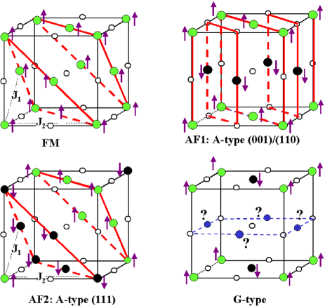
Figure 1: (Color on-line) Magnetic phases used for the Heisenberg model fit: FM; AF₂ that is built of alternating (111) planes of like spins [highlighted by thick (red) lines]; AF₁, made of alternating (011) (or equivalently (001)) planes of like spins, delimited by (red) thick lines. The highly frustrated G-type AF phase is also shown for comparison. Filled light (green, up spin) and black (down spin) circles indicate TM atoms, small empty circles are for oxygens. For the G-type phase (blue) filled circles marked with a question mark indicate TM atoms with frustrated spin direction.

In order to evaluate J₁ and J₂ we need to consider at least two competing high-symmetry magnetic phases beside the observed AF₂. Natural choices are the ferromagnetic (FM) order and the AF (110) A-type order with (110) spin-paired planes compensated along [110] (labeled AF₁). AF₁ can also be seen as made of FM (001) planes alternating along [001] (see Fig. 1). The AF₁ phase has all the 6 NNN spin-paired, 4 of the NN spin-paired, and 8 NN spin-antipaired. On the other hand, it is interesting to note that the G-type AF order (also depicted in Fig. 1) is strongly disfavored by frustration, since in FCC symmetry there is no way to arrange the 12 NN interactions in antiparallel fashion without conflict.

To extract J₁ and J₂ we fit our calculated total energies to a standard 2-parameter classical Heisenberg Hamiltonian of the form:

$$H=-J_{1}\sum_{\langle i,j\rangle}\vec{e_{i}}\cdot\vec{e_{j}}-J_{2}\sum_{\langle\langle i,j\rangle\rangle}\vec{e_{i}}\cdot\vec{e_{j}}$$ (11)

where $\langle i,j\rangle$ and $\langle\langle i,j\rangle\rangle$ indicate summation over NN and NNN, respectively, and $\vec{e_{i}}$ is the spin direction unit vector. Energies (per f.u.) are then expressed as:

$$E_{FM} = E_{0}-6J_{1}-3J_{2}$$

$$E_{AF_{1}} = E_{0}+2J_{1}-3J_{2}$$

$$E_{AF_{2}} = E_{0}+3J_{2}$$ (12)

This is solved to give:

$$J_{1} =\frac{1}{8}(E_{AF_{1}}-E_{FM})$$

$$J_{2} =\frac{1}{24}(4E_{AF_{2}}-3E_{AF_{1}}-E_{FM})$$ (13)

With this choice of the Hamiltonian, negative and positive J values correspond to energy gain for spin-antiparallel and spin-parallel orientations, respectively.

Finally, we mention that several other anisotropic terms may in principle contribute to the Heisenberg Hamiltonian, related to short-range dipolar interactions favoring a preferential spin direction parallel to (111) planes, and to rhombohedral distortions of the AF₂ phase consisting on a (111) inter-planar contraction and slight change of the perfect 90^∘ angle of the rock-salt cell, which causes a symmetry breaking of J₁ in two J${}_{1}^{+}$ and J${}_{1}^{-}$ values.franchini However, all these effects are quantified to be order-of-magnitude smaller than the dominant exchange-interaction energies (e.g. for NiO J${}_{1}^{+}$-J${}_{1}^{-}$ $\sim$ 0.03 meV according to neutron datahutchings ), thus the Heisenberg Hamiltonian written in Eq.11 can be considered fully sufficient for our present purposes.

IV Results

IV.1 Equilibrium structures

We have calculated total energies and pressures of MnO and NiO as a function of lattice parameter for the 3 magnetic phases FM, AF₂, and AF₁. Values of the equilibrium lattice parameter and bulk modulus for the stable AF₂ phase are reported in Table 1, in comparison with the experimental values.

Table 1: Equilibrium lattice constants a₀ (in Å) and bulk moduli B₀ (in GPa) calculated in this work with various methods, compared with experimental values. All values refer to the stable AF₂ magnetic ordering.

	LDA-PW	PSIC	LDA-LO	ASIC	PBE	HSE	Expt.
MnO
a0	4.38	4.35	4.35	4.35	4.47	4.41	4.43a
B0	158	194	177	199	145	170	151b,162c
NiO
a0	4.15	4.09	4.09	4.06	4.19	4.18	4.17d
B0	234	269	270	287	183	202	180-220e
a): Ref.sasaki, ; b): Ref.noguchi, , c): Ref.jeanloz,
d): Ref.schmahl, ; e): Ref.huang,

Results are quite satisfactory overall: each method predicts an equilibrium lattice constant in good agreement (within 1-2%) with experiment for the AF₂ phase. It is well known that structural properties calculated by LDA or GGA can be good, or even excellent, although the electronic properties are poor.marsman ; franch07 The results for MnO and NiO are a case in point, as both LDA-PW and PBE stay within 1% from the experiment (the former in defect, the latter in excess), while the LDA-LO result is about 2% below the experimental value. As for beyond-local functionals, HSE sllightly underestimates PBE results and as a consequence is quite close to experiment, while PSIC and ASIC underestimate their respective local-functional (LDA-PW and LDA-LO) references by $\sim$1% on average (a tendency also foundvpsic in other classes of oxides such as titanates and manganites).

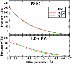
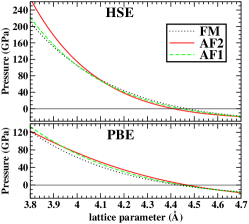
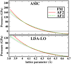
Figure 2: (Color on-line) Calculated pressure for MnO in the three considered magnetic phases (see text). Each panel reports results obtained by a different energy functional or methodology considered in this work.

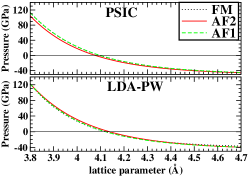
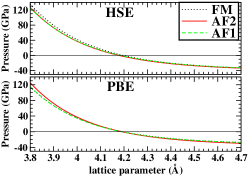
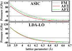
Figure 3: (Color on-line) Calculated pressure for NiO in the three considered magnetic phases (see text). Each panel reports results obtained by a different energy functional or methodology considered in this work.

In Figs. 2 and 3 the calculated pressures for, respectively, MnO and NiO are reported as a function of lattice parameters for the three magnetic phases. The behavior in the region around the equilibrium lattice constant is expressed by the calculated bulk modulus (B₀) in Tab.1. The advanced functionals coherently give an increase of B₀ by $\sim$20-30 GPa ($\sim$15%) with respect to their respective local functionals. This increase is a consequence of the enhanced 3d state localization and concomitant increase in Coulomb repulsion under compression which is expected from beyond-local approaches. Concerning the agreement with experiment, both PBE and HSE give values within the reported experimental uncertainty. In contrast, LDA-PW gives B₀ at the higher end of the experimental error bar, thus that the 15% further increase caused by PSIC pushes the value of B₀ $\sim$40-50 GPa above the experiment. Hence the discrepancy should be seen as due to the LDA-PW performance (and to the characteristics of the used pseudopotentials), rather than as a failure of the PSIC method in itself. This trend can also be observed for the local orbital basis, where the LDA results for B₀ are already slightly above the the experimental values, and the addition of the ASIC corrections simply pushes the bulk modulus further away.

A very interesting feature which emerges consistently from all the methods is the quite similar pressure dependence for different magnetic orderings, especially evident for NiO. This looks surprising at first glance, especially at strong compressive pressure, where (as discussed later on) changes in the magnetic ordering are related to metal-insulating transitions and to radical changes in the electronic properties. The explanation is that $e_{g}$ electrons (strongly hybridized with O $p$ states) govern the electronic and magnetic properties, but have only a minor effect on the response to applied hydrostatic pressure. In MnO, where $t_{2g}$ states are also magnetically active, pressure is slightly more sensitive to the specific magnetic ordering (in Fig.2 AF₂ tends to differ from AF₁ and FM, which almost overlap each other). It should also be noted that in MnO for very contracted lattice constants the advanced functionals give pressures a factor of 1.5-2 larger than those of the corresponding local functionals, depending on the method and specific magnetic phase. At variance, for NiO advanced and local functionals give pressures in the same range. This reflects the larger effect of the advanced functionals on the half-filled $t_{2g}$ shell of MnO, which is pushed down in energy and increase its spatial localization and its Coulomb repulsion under compression, than on the filled $t_{2g}$ shell of NiO.

IV.2 Magnetic properties upon applied pressure

IV.2.1 Magnetic phase diagram under pressure

Figs. 4 and 5 summarize our findings concerning phase stability and magnetic moments for MnO and NiO. Each panel reports results obtained by a given energy functional for relative magnetic energies (with respect to the most stable magnetic ordering) and their corresponding magnetic moments, as a function of lattice constant. Column-wise, panels are ordered according to the code used: LSDA-PW and PSIC results (left, PWSIC); PBE and HSE results (center, VASP); LSDA-LO and ASIC results (right, SIESTA).

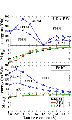
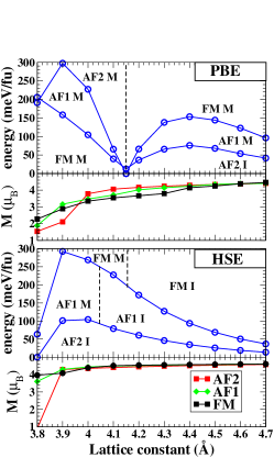
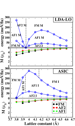
Figure 4: (Color on-line) Total energies (relative to the ground state) and magnetic moments of FM, AF₁ and AF₂ phases of MnO as a function of lattice parameter, calculated by LDA-PW and PSIC (left panels), PBE and HSE (center panels), LDA-LO and ASIC (right panels). The insulating (I) or metallic (M) character of each magnetic phase is also indicated. Vertical dashed lines indicate phase transitions.

We start our analysis from MnO results given by LDA-PW, LDA-LO, and PBE (top panels of Fig.4). We can capture immediately the substantial similarity of the three approaches: at large volumes all have a region where AF₂ is the most stable phase and insulating, a metallic AF₁ region $\sim$50-100 meV above AF₂, and a metallic FM region $\sim$100-150 meV above AF₂. Going from large- to small-lattice region, all three methods reports a phase transition (indicated by the vertical dashed lines) through which the AF₂ phase yields to a metallic FM region as ground state, which wins over higher-energy AF₁ and (further above) AF₂ metallic phases. The critical value of lattice parameter corresponding to the transition differs in the three approaches 4.3 Å  in LDA-PW, 4.15 Å  according to PBE, and 3.9 Å  for LDA-LO. Looking at the corresponding magnetic moments, LDA-PW and PBE show a similarly gradual moment decay when going from 4.7 Å  up to a threshold of 4.0 Å  (LDA-PW) and 4.1 Å  (PBE), corresponding, in the pressure scale, to$\sim$40 GPa and 80 GPa, respectively. Below this threshold, magnetic moments fall quite abruptly down to $\sim$ 2 $\mu_{B}$ at 3.8 Å  for the stable FM metallic phase (notice that this unphysical collapse described by LDA-PW and PBE is not related to the true moment collapsecohen in MnO at much higher pressures). At variance, moments calculated by LDA-LO decay gradually through the whole lattice constant range, without collapsing as in LDA-PW and PBE. This difference reflects the persistence of the AF₂ stability in a larger parameter range described by LDA-LO.

Now we analyze the results obtained within beyond-local functionals. Overall, the picture is radically different: for the whole range of lattice parameters, the AF₂ insulating phase is robustly the ground state, and the spurious phase transition discussed above is absent. Furthermore, all three approaches coherently report a stability enhancement (i.e. a roughly linear energy gain) of AF₂ for decreasing lattice constant. This effect is indeed expected as a consequence of the increased Mn $d$-O $p$ covalency and the related strengthening of AF superexchange coupling. The AF₂ maximum stability is reached at $\sim$3.9 Å  according to PSIC (corresponding to an applied compression of $\sim$130 GPa), at $\sim$4.0 Å  for ASIC (P$\sim$130 GPa) and HSE (P$\sim$90 GPa). The peak of AF₂ energy gain with respect to the equilibrium structure is nearly 100%, from $\sim$50 meV/f.u. to more than 100 meV/f.u. according to HSE and PSIC. Above AF₂ all our advanced functionals favor the AF₁ phase, that, at variance with the always insulating AF₂ phase, undergoes a metal-insulating transition at 3.97 Å  (PSIC), 3.95 Å  (ASIC) or 4.05 Å  (HSE). Above AF₁ resides a FM region, again separated in a large-volume insulating and small-volume metallic sides, with an insulating-metal transition threshold of 4.07 Å  for PSIC, and 4.15 Å  for both ASIC and HSE. This consistency is also reflected in similar values of magnetic moments through the whole lattice constant range: all methods describe a moderate decline from $\sim$ 4.7 $\mu_{B}$ at 4.7 Å  to $\sim$ 4.0-4.2 $\mu_{B}$ (depending on the specific magnetic phase) at $a$=3.8 Å.

Interestingly, the remarkably coherent picture delivered by our advanced functionals for MnO is not limited to the predict the same ground-state, but also involves ordering and energy differences among the three magnetic phases. This is instrumental to coherently describe finite-temperature properties as well, as shown in Section IV.2.3.

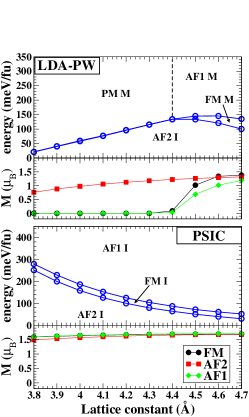
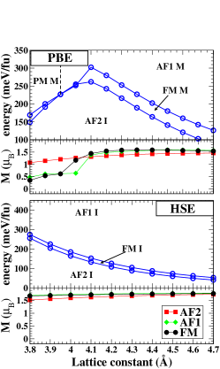
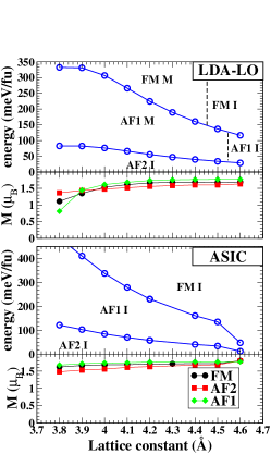
Figure 5: (Color on-line) Total energies (relative to the ground state) and magnetic moments of FM, AF₁ and AF₂ phases of NiO as a function of lattice parameter, as calculated for the different methods used in this work: LDA-PW and PSIC calculations (left), PBE and HSE calculations (center), LDA-LO and ASIC calculations (right). PM indicates Pauli Paramagnetic ordering, I and M insulating and metallic character, respectively. Vertical dashed lines indicate phase transitions.

Now we move to the analysis of NiO results, summarized in Fig. 5, starting again from the phase stability diagram drawn by the three local functionals (upper panels). At variance with what seen for MnO, now all the methods give the insulating AF₂ phase as stable at any lattice constant; however the competition with the other two orderings is described differently: according to LDA-PW, moving from large to small lattice constants there is first a tiny region where the AF₂ stability increases, reaches maximum at 4.4 Å  (thus much above the equilibrium value) and then start falling linearly all the way down to 3.8 Å . Furthermore, above AF₂ the LDA-PW predicts a coexistence of degenerate AF₁ and FM metallic phases. This scenario can be rationalized looking at the magnetic moments for AF₁ and FM calculated in LDA-PW: starting from the large lattice constant value of $\sim$ 1 $\mu_{B}$, the magnetic moment falls rapidly and vanishes altogether just at 4.4 Å  (i.e. still above the equilibrium value of 4.35 Å). Below this threshold the LDA-PW describes a metallic, Pauli paramagnetic region. On the other hand, the expected Mott-insulating behavior is only maintained in the AF₂ phase. This feature represents a major shortcoming which seriously hamper the NiO description by LDA-PW.

PBE shows a similar, although slightly less dramatic failure, since the moment collapse starts to show up for smaller lattice constant values (4.0 Å  for FM and 4.1 Å  for AF₁, thus definitely below the equilibrium 4.19 Å ), and the magnetic moment is severely reduced to about 0.5 $\mu_{B}$, without vanishing completely. Quite distinct is the behavior of LSDA-LO, which shows two well energy-separated phases, AF₁ above AF₂, and then FM further above, both undergoing metal-insulating transitions when moving from smaller to larger lattice parameters. This peculiarity is clearly reflected in the calculated magnetic moment: there is no collapse at least until 4.0 Å , then a rapid downfall starts, but the moments remain quite sizable up to 4.0 Å , at variance with what seen for PBE and LSDA-PW, and consistently with what is found for MnO as well. This signals the tendency of LDA-LO to conserve sizable Mott gap and magnetic moments in a range of lattice parameters where plane-wave based implementations describe the system as already collapsing to metallic paramagnets (as explicitly shown later on in the DOS analysis).

Moving to the analysis of beyond-LDA functionals, all of them consistently predict the large enhancement of AF₂ stability upon lattice constant decrease in a wide range around the equilibrium value. The artificial moment collapse described by the local functionals is absent, and all the magnetic phases remain insulating through the whole lattice constant range. All methods find magnetic moments of about 1.7-1.8 $\mu_{B}$ at large lattice constants, and a very moderate decrease to $\sim$1.5 $\mu_{B}$ at the smallest lattice constant considered (3.8 Å). Particularly striking is the agreement between HSE and PSIC, both describing a tiny FM region intermediate between AF₂ and AF₁, and a parabolic rise of the AF₂ energy gain from $\sim$50 meV at 4.7 Å  up to $\sim$250 meV at 3.8 Å. On the other hand, ASIC gives a different phase ordering (AF₂-AF₁-FM), with a smaller increase of the AF₂ relative stability from $\sim$0 meV at 4.7 Å  to $\sim$120 meV at a=3.8 Å.

In order to clarify the difference in the magnetic moments under pressure obtained by the different methods, we have calculated the orbital-resolved density of states (DOS) for NiO at two representative lattice constants, $a$=4.5 Å  and $a$=4.0 Å , corresponding to situations of tensile and compressive strain. The results are shown in Fig. 6.

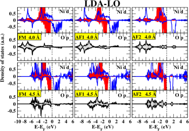
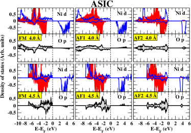
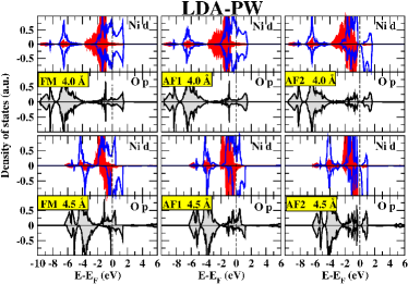
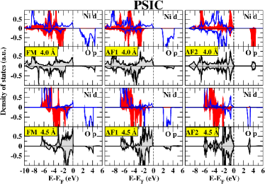
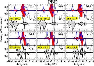
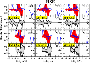
Figure 6: (Color on-line) Orbital-resolved DOS for NiO calculated at two lattice constant values (4.0 Å, and 4.5 Å) with all our employed functionals: LDA-LO (top left), ASIC (top right), LDA-PW (middle left), PSIC (middle right), PBE (bottom left) and HSE (bottom right). Only the DOS for the relevant orbitals are shown: O p (filled gray curves) and Ni d, separated in t_2g (filled red curves) and e_g (solid blue lines) contributions. Positive and negative curves represent majority and minority contributions.

Starting from the local-functional results at 4.0 Å, we notice a radical difference between the two LDA implementations. LDA-LO predicts a metallic ground state for both the FM and AF₁ phases, with sizeable $e_{g}$ spin-splitting and substantial magnetic moments on Ni, whereas the AF₂ phase is found insulating, with a $\sim$1 eV energy gap. On the other hand according to LDA-PW FM and AF₁ phases are Pauli-paramagnetic, with perfectly compensated spin-densities, while in the AF₂ phase a barely visible gap opens up within the $e_{g}$ manifold. PBE results stand somewhat in the middle of the previous two descriptions: for FM and AF₁ some Pauli magnetization shows up in the upper $e_{g}$ manifold, while for AF₂ the magnetic moment is formed, and a Mott gap is about to open. Even at $a$=4.5 Å  some differences among the local functionals are detectable: according to LDA-LO a minimal gap is opened for each phase, while for LDA-PW only the AF₂ is insulating. PBE provides well formed magnetic moments in each phase but only AF₂ is clearly insulating.

Going to the results for beyond-local functionals, the expected picture of wide-gap intermediate charge-transfer/Mott insulator described by the experimentsschuler ; shukla ; kunes2 is restored. Now the DOS is that of a robust insulator under both lattice expansion and compression, with a valence band top populated by a mixture of O p and Ni d states, and the conduction bottom with a majority of e_g and a minor fraction of O p states. The energy gap for the AF₂ phase ($\sim$3 eV for ASIC and $\sim$3.5 eV for both PSIC and HSE) is in good agreement with the experimental value, and even FM and AF₁ phases show sizeable gaps of about 1-2 eV. Overall, the similarity of spectral redistributions for $e_{g}$, $t_{2g}$, and O $p$ states (especially for HSE and PSIC) is remarkable.

In summary, for both MnO and NiO beyond-local functionals deliver a very coherent description of relative phase stabilities in the whole examined range of lattice parameters, and predict a clear enhancement of the AF₂ phase relative stability (not described by local functionals) within a wide lattice parameter interval, which suggests the possibility of an enhancement of the magnetic ordering Néel temperature (T_N) upon applying compressive stress. Before exploring the validity of this expectation we will first discuss the evolution of the magnetic coupling constants upon compression.

IV.2.2 Exchange interactions under pressure

A few qualitative considerations on magnetic interactions can help to correctly interpret our results. Our calculations find the T=0 magnetic ground state to be the observed AF₂ for both MnO and NiO; however, the detailed magnetic interactions suggest two different scenarios. Magnetic coupling between Mn²⁺ 3$d^{5}$ ions is mediated by half-filled orbitals (thus J₁ mainly by $t_{2g}$-$t_{2g}$ and J₂ by $e_{g}$-$e_{g}$ couplings), which are both robustly AF oriented according to superexchange theory.anderson59 ; GoodenoughKanamori Thus we expect J₁ and J₂ to be both sizable and negative (i.e. AF in our present convention). For Ni²⁺ $d^{8}$ ions, on the other hand, only $e_{g}$-$e_{g}$ coupling is magnetically active. Hence we expect a large and negative J₂ due to the dominance of covalent superexchange, very small and positive J₁ due to superexchange-mediated 90^∘-oriented $e_{g}$-(O $p_{x}$,$p_{y}$)-$e_{g}$ orbital coupling, and therefore huge J₂/J₁ values.

These expectations are largely confirmed by our results: in MnO (Fig.7) J₁ and J₂ roughly track each other as function of the lattice parameter irrespective of the calculation method. However, it is of the utmost importance to observe the dramatic difference between the description of local and advanced functionals: looking at LDA-PW results [panel a)] J₁ and J₂ are moderately negative at expanded lattice, then upon lattice shrinking they both change sign and grow up to a maximum value at $\sim$ 4 Å, and finally fall back down as the lattice shrinks further. The PSIC almost completely reverses this behavior: J₁ and J₂ nearly vanish at 4.7 Å  (signaling a shorter interaction range with respect to LDA), and then grow steadily (in absolute value) on the negative side as the lattice squeezes up. Curiously, LDA-PW and PSIC curves intersect each other at $\sim$ 4.4 Å, but this agreement near the equilibrium lattice is just a fortuitous crossing of two otherwise radically different behaviours. Notice finally that while in PSIC J₂/J₁$>$1 at any lattice parameter, in LDA-PW the exchange interaction ratio fluctuates as function of the lattice constant.

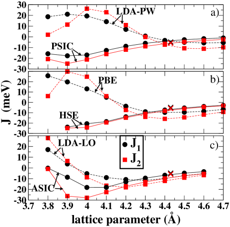
Figure 7: (Color on-line) Exchange-interaction parameters J₁ (black filled circles) and J₂ (red filled squares) as a function of lattice parameter calculated for MnO with various approaches. From top to bottom: a) with PWSIC code by LDA-PW and PSIC functionals; b) with VASP code using PBE and HSE functionals; c) with SIESTA code using LDA-LO and ASIC functionals. Dashed lines refer to local density functional (LDA-PW, PBE, LDA-LO) calculations, solid lines represent beyond-local density functionals calculations (PSIC, HSE, and ASIC). Black and red crosses show experimental values for J₁ and J₂, respectively, reported for MnO in Table 2.

The considerations exposed for LDA-PW and PSIC can be identically repeated for PBE and HSE, respectively (the similarity of curves is apparent comparing panel a) and b) in Fig.7). The behavior of LDA-LO [panel c)] is more peculiar: as previously noticed, the local-orbital implementation seems to cure, though only partially and perhaps accidentally, already at the LDA level some of the deficiencies of the local functionals related to the self-interaction problem. It turns out indeed that the exchange interactions determined by LDA-LO show characteristics similar to those depicted by the non-local functionals: at large lattice parameter both J₁ and J₂ are vanishing and negative, then they correctly grow negative upon lattice shortening up to 4.2 Å(thus well below the equilibrium structure), but then they revert slope and turn positive below 4.0 Å. The ASIC, on the other hand, restores through the whole lattice range the correct description already seen for PSIC and HSE.

Now we move to examine NiO (Fig.8). As expected, the relative weight of J₁ and J₂ is very different: all functionals (both local and beyond-local) describe J₁ as very small and positive at any lattice value (black symbols). On the other hand, the large and negative J₂ is again differently described by the two sets of functionals. For LDA-PW/PBE and PSIC/HSE (Fig.8) we can repeat most of the considerations made for J₂ in MnO: the behavior with lattice parameter is roughly inverted, although the two curves crosses at different values of the lattice constant (4.2 Å  for LDA/PSIC, 3.9 Å  for PBE/HSE). LDA-LO is again a case in its own, as it appears to provide results not far from the ASIC ones in the lattice region above 4.2 Å. ASIC qualitative behavior for both J₁ and J₂ is in line with that of PSIC and HSE, although its J₂ appears amplified by nearly a factor 2. In consideration of what we have seen so far, the reason of this difference seems to reside more in the methodology (i.e. technical implementation: plane wave versus atomic orbitals) rather than in the employed functional.

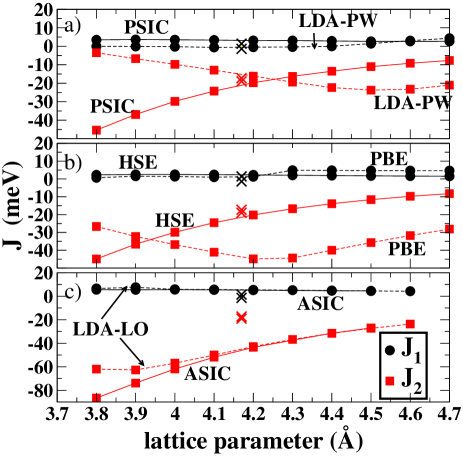
Figure 8: (Color on-line) Exchange-interaction parameters J₁ (black filled circles) and J₂ (red filled squares) as a function of lattice parameter calculated for NiO with various approaches. From top to bottom: a) with PWSIC code by LDA-PW and PSIC functionals; b) with VASP code using PBE and HSE functionals; c) with SIESTA code using LDA-LO and ASIC functionals. Dashed lines refer to local density functionals calculations (LDA-PW, PBE, LDA-LO), whereas solid lines represents beyond-local density functionals calculations (PSIC, HSE, and ASIC). Black and red crosses show experimental values for J₁ and J₂, respectively, reported for NiO in Table 2.

From a phenomenological viewpoint, it is important to note the appreciable growth of the exchange interactions for decreasing lattice parameter in a wide region extending well below the equilibrium value (i.e. for large applied compression), coherently described by all our beyond-local functionals. In the next section we will illustrate the remarkable reverberations of this behavior on the magnetic ordering temperature. For now, we remark that this is the expected behavior of the so called covalent exchange, i.e. the shorter the TM-O distance, the stronger the energetic advantage for the O 2$p$ ligand states to overlap with the adjacent TM 3$d$ states with unlike spins. This advantage reaches a maximum at a certain compression, after which the J’s start falling. This is the point when the pressure is so strong that minority DOS begins to be appreciably populated and in turn magnetic moments start falling.

Overall, the comparative analysis of the three beyond-local functionals is very satisfying, as they furnish a qualitatively and quantitatively coherent and physically sound description of exchange interactions under pressure for MnO and NiO. There is a large body of data in literature, both theoretical and experimental, with which to compare our data, at least at equilibrium. In Table 2 we report our values for the theoretical equilibrium structure in comparison with the experimental values and other theoretical predictions obtained by several density functional based approaches (see Section I; we neglect tight-binding or shell-model results, which rely on experimental fitting).

The J’s reported in the Table are determined by finite energy differences, unless otherwise specified. In some cases, the magnetic force theorem (MFT)liechtenstein based on the exchange-correlation density-functional gauge invariance under infinitesimal spin rotationssolovyev ; vignale was used. In Ref.kotani, , exchange interactions and the whole spin-wave spectrum was determined from the poles of spin susceptibility.savrasov ; karlsson As for experiments, results from both inelastic neutron scattering (INS)kohgi ; hutchings and thermodynamic data (TD)lines ; shanker are reported.

Comparison of J values given by different approaches and considerations on the level of agreement with the available experimental data must be taken very carefully. Differences of the order of a few meV may derive from technical implementation aspects rather than from the basic theory itself, as testified by the sizable difference of results obtained by the same theory in different calculations (e.g. our LDA-LO and LDA-PW). Concerning MnO, the comparison is further complicated by the close similarity of the two J values. It is expected that local functionals should overestimate the J’s, due to the underestimation of intra-atomic exchange splitting and the related overestimation of $p$-$d$ hybridization. This is indeed verified with LDA-LO and PBE. Notice, however, the relevant exception of LDA-PW (overall, the least accurate of the three local functionals) which deliver J’s in excellent agreement with the experiment: this fortuitous agreement was previously explained as consequence of the unphysical AF₂ to FM transition occurring in LDA-PW near the equilibrium structure. On the other hand, our beyond-local functionals perform quite satisfactorily, apparently ranking among the closest to experiment both in absolute terms and concerning the J₂/J₁ ratio (1.16 for INS data, 1.1 for HSE, 1.4 and 1.5 according to ASIC and PSIC).

For NiO the analysis is simpler, as J₁ is very small and a qualitative comparison can be done on the base of J₂ only. We have already commented that the LDA-PW is grossly inadequate, thus it can be left aside. As for LDA-LO and PBE, they deliver sizably overestimated J₂. As for beyond-local functionals, we have previously seen that that J’s calculated by PSIC and HSE almost overlap each other throughout the lattice parameter range. The agreement with values drawn from neutron experimentshutchings is indeed quite satisfying. Nevertheless, the slight PSIC underestimation of the equilibrium lattice parameter (4.09 Å  against the near experimental-matched 4.18 Å  of HSE) reverberates in a $\sim$15% overestimation of J₂. On the other hand, ASIC delivers J’s that barely differ from the corresponding LDA-LO values, and are amplified by nearly a factor 2 with respect to PSIC and HSE. Looking at previous literature, we found a substantial agreement of PSIC and HSE with GGA+U calculations of Ref.zhang, (here the J’s are also calculated as a function of lattice parameter) and with other types of hybrid functionalsmoreira as well. On the other hand, both unrestricted HFmoreira , full SIC in LMTO approach (SIC-LMTO)kodde and the local SIC (LSIC) (a KKR-based implementation of the self-interaction correction methodhuges ; dane ; fischer ) tend to an excessive electronic localization, which thus turns into a slight underestimation of the exchange interactions.

Table 2: Exchange interaction parameters for MnO and NiO (in meV) calculated in this work, compared to experimental and theoretical values from previous works.

	MnO				NiO
	J1	J2			J1	J2
Experiment
INSa	-4.8	-5.6		INSb	1.4	-19.0
TDc	-5.4	-5.9		TDd	-1.4	-17.3
This work: local functionals
LDA-PW	-2.7	-6.3		LDA-PW	-0.5	-14.7
LDA-LO	-10.6	-13.6		LDA-LO	5.4	-43.5
PBE	-9.5	-14.9		PBE	1.2	-44.5
This work: advanced functionals
PSIC	-5.0	-7.6		PSIC	3.3	-24.7
HSE	-7.0	-7.8		HSE	2.3	-21.0
ASIC	-8.0	-11.3		ASIC	5.2	-45.0
Previous calculations
LSDAe (MFT)	-13.2	-23.5
LDA+Ue (MFT)	-5.0	-13.2		GGA+Ul	1.7	-19.1
OEPe (MFT)	-5.7	-11.0		SIC-LMTOm	1.8	-11.0
PBE+Uf	-4.4	-2.3		Fock-35n	1.9	-18.7
PBE0f	-6.2	-7.4		B3LYPn	2.4	-26.7
HFf	-1.5	-2.32		UHFn	0.8	-4.6
QPGWg	-2.8	-4.7		QPGWg	-0.8	-14.7
LSICh	1.4	-3.3		LSICh	2.8	-13.9
LSICh (MFT)	-1.8	-4.0		LSICh (MFT)	0.3	-13.8
B3LYPi	-5.3	-11.0
a): Ref.kohgi, , b): Ref.hutchings, , c): Ref.lines, d): Ref.shanker,
e): Ref.solovyev, , f): Ref.franchini, , g): Ref.kotani, , h): Ref.fischer,
i): Ref.feng, , l): Ref.zhang, , m): Ref.kodde, , h): Ref.moreira,

IV.2.3 Critical transition temperatures under pressure

Fig. 9 reports critical temperatures for MnO and NiO calculated with the Heisenberg Hamiltonian given in Eq.11 and solved through classical MonteCarlo (MC) simulated annealing technique.mc Values calculated at equilibrium and at experimental volume are reported in Tab. 3, in comparison with the experiment and other theoretical predictions.

We start discussing the case of MnO as described by our local density functionals. As expected, MC calculations describe fictitious phase transitions (consequence of the spurious magnetic moment collapse previously discussed) from AF₂ to FM metallic magnetic phase (highlighted by the dashed areas) while moving from large to small lattice parameters. The onset of this transition depends on the method: it is especially harmful in LDA-PW as it occurs near (just below) the theoretical lattice value (4.35 Å); much less damaging in LDA-LO, where it happens at a much larger lattice contraction (4 Å); PBE is halfway the two previous cases. In all cases this phase transition dramatically alters the critical temperature behavior, which is expected to grow (at least in some interval around equilibrium) as the lattice parameter contracts. Furthermore in all cases the predicted T_N (see Tab. 3) remains quite distant from the experimental T_N=118 K (horizontal dashed line in the Figure). Notice again that while LDA-LO and PBE overestimates T_N at the equilibrium structure, the spurious phase transition in LDA-PW cause T_N to be smaller than the experimental values, and paradoxically not too far (at experimental lattice constant) from the experiment. This is another manifestation of the fortuitous agreement already pointed out in the illustration of the exchange interactions.

Conversely, the advanced functionals deliver for MnO a nicely consistent picture, with T_N growing steadily from very large lattice constants (T_N $\rightarrow$0) up to 3.9-4.0 Å, and peaking at $\sim$410 K (PSIC and HSE) or 480 K (ASIC). The corresponding pressure is around 120$\pm$20 GPa depending on the approach (see Fig.2). There is a minor offset between the three methods, due to the slight increase in J’s moving from PSIC to HSE to ASIC. However, if calculated at their respective equilibrium values, both PSIC and HSE predict a T_N which is almost spot-on to the experimental value.

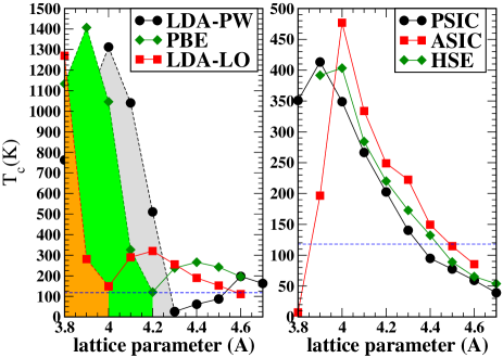
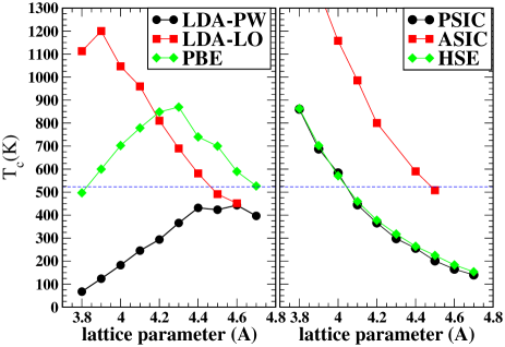
Figure 9: (Color on-line) Critical temperatures as a function of lattice constant for MnO (top panel) and NiO (bottom) calculated by simulated-annealing MonteCarlo simulation of the Heisenberg Hamiltonian in Eq.11. Left and right panels separate local and advanced functionals used to determine each set of (J₁, J₂). The shaded areas in the top-left panel indicate FM metallic regions; apart from that, each curve separates low-T insulating AF₂ from high-T insulating PM regions (PM stands for Pauli Paramagnetic ordering). The dashed horizontal lines indicate experimental T_N values.

Moving to the analysis of NiO, the three local functionals behave quite differently from each other, although PBE and LDA-LO fortuitously cross nearby the equilibrium value. So, it is all the more remarkable that their beyond-local counterparts are capable to rebuild a very consistent picture, with T_N linearly growing along with the decrease of lattice parameter. The near-overlap of HSE and PSIC is especially striking, and already noticed for the J’s. The ASIC curve appears translated upward by nearly a factor 2, coherently with the overestimate of the dominant J₂ value. Notice that for NiO there is no lattice parameter turning point in the considered range, thus T_N keeps growing up to 3.8 Å, corresponding to a pressure of about 100-120 GPa (see Fig.3). The agreement with the experiment for NiO is much less outstanding than for MnO, as both HSE and PSIC remains below the experimental T_N=523 K by $\sim$20% (at the equilibrium structure the PSIC value is actually not too far from the experiment thanks to its underestimated lattice parameter), while ASIC is close to the much overestimated LDA-LO value.

The disagreement between ab initio theoretical estimates and the experimental value of T_N for NiO is typical and well documented in literature (see e.g. Ref.fischer, and references therein) and a full discussion on the subject is beyond our present scope. We only remark that the mismatch with HSE and PSIC is somewhat puzzling, in consideration of the excellent agreement of the calculated J₂ with the experimental value. In fact, even using experimental sets of J’s, the MC-calculated T_N would change only marginally our theoretical value: as a useful reference we also report in the Table the T_N of MnO and NiO calculated by MC using sets of experimental J’s reported in Table 2. It turns out that these T_N underestimate by $\sim$ 30% the directly measured T_N (they are even lower than those obtained with our calculated J’s, since the slight overestimation of our calculated J’s helps in shifting up the predicted T_N). The discrepancy between experimental J’s and T_N somewhat points out to possible inadequacies of the employed Heisenberg model, possibly due to further terms (not included in Eq.11) which might be important at the relatively high ordering temperature of NiO.

In Tab.3 we compare our results with some previous theoretical predictions (we omit the many mean-field approximations which are known anderson59 to grossly overestimate the critical temperature). Ref. fischer, proposes T_N obtained by disordered local moments (DLM), random-phase approximations (RPA) and MC, based on the MFT-calculated J’s given in Table 2. The DLM values are closest to our HSE and PSIC estimate, while RPA and MC values for NiO are larger than our values despite smaller J’s, due to the debatable inclusion in Ref.fischer of the quantum rescaling factor (S+1)/S.wan Ref.wan, also proposes MFT-calculated J’s, derived from LDA, LDA+U, and LDA plus dynamical mean field approach solved through cluster exact diagonalization (CED). The latter seems to restore an outstanding agreement with the experimental T_N for NiOnote .

Table 3: Critical temperatures (K) for MnO and NiO calculated in this work at equilibrium and experimental (in brackets) lattice constant, compared with experimental (neutron diffraction, ND) and theoretical values from previous works. As a reference we also report MC-calculated values obtained by using the experimental J’s (see text for discussion).

	MnO	NiO
Experiment
NDa,b	118	523
Expt. J’s	85c	340d
Expt. J’s	90e	300f
This work: local functionals
LDA-PW	55 (71)	272 (280)
LDA-LO	220 (176)	967 (851)
PBE	249 (257)	824 (829)
This work: advanced functionals
PSIC	116 (89)	458 (387)
HSE	125 (116)	393 (400)
ASIC	182 (137)	1048 (850)
Previous works
LSICg (DLM)	126	336
LSICg (RPA)	87	448
LSICg (MC)	90	458
LDAh (MC)	423	965
LDA+Uh(MC)	240	603
CEDh (MC)	172	519
a): Ref.roth, , b): Ref.shull, , c) Ref.kohgi, , d) Ref.hutchings, , e) Ref.lines, .
f) Ref.shanker, , g) Ref.fischer, , h) Ref.wan, .

V Summary and Conclusions

It is fair to affirm that the overall account of the structural, electronic, and magnetic properties of MnO and NiO provided by the advanced functionals is overall quite satisfying, internally consistent, and in good agreement with experiments. In particular, HSE shows a remarkable quantitative agreement with experiments on most examined properties; the PSIC, perhaps surprisingly when considering the substantially different conception at the basis of their theoretical constructions, is quite comparable with HSE results, and in some cases in spectacular quantitative agreement (e.g. the NiO exchange interactions vs. lattice constant). An important persistent shortcoming of PSIC or ASIC, however, is the prediction of structure: the predicted lattice constant is below experiment by $\sim$1-2%. This tendency to deliver smaller-than-optimal structural parameters was also encountered in other situationsvpsic , and it is probably not an isolated occurrence, but rather a characteristics of the PSIC/ASIC method. In perspective, we expect that this drawback could be overcome by adopting the GGA (e.g. PBE) instead of the LDA as reference functional upon which to build the PSIC projector (see Refs.fs, ; ff-coll, for details). This would probably lead, as in the case of HSE, to a moderate volume reduction compared to the slightly overestimated GGA volume, hence probably to an end product much nearer to experiments.

Some additional considerations concern the comparison of different implementations of the same theory, i.e. LDA-PW vs. LDA-LO and PSIC vs. ASIC. Interestingly, some visible quantitative differences appear already at level of local functionals. Hence, these are not induced by the ASIC/PSIC formulation, which in fact tends to re-equalize the respective descriptions. The amplitude of the PSIC vs. ASIC discrepancy is only minor for MnO, and a bit more pronounced for NiO, especially concerning the amplitude of J₂. This is not particularly surprising, since different choices of local orbital basis set and/or pseudopotentials can easily alter meV-scale quantities. In fact we can find in the literature a wide spread of values for exchange interactions predicted by different implementations of the same theory (even at the LDA level). Not by chance the different basis set has more impact on NiO exchange interactions than in the MnO ones, since the e_g charge spreads more in space than the highly localized t_2g one, and as such it is clearly more sensitive to the incomplete description of the intersticial space due to local orbital basis. As a trade off, this larger error bar is compensated by the ASIC capability to tackle large-size systems (up to a few thousands atoms) which in fact are impracticable for the, in principle, more accurate plane-wave approaches such as PSIC and HSE. A valuable testing ground of this capability may be the field of oxide interfaces, where a plethora of new exciting phenomena have been recently discovered. It will be interesting to evaluate whether PSIC/ASIC or HSE are capable to describe e.g. composite systems such as an interface between a metal and insulator, where the degree of charge localization at the two sides is rather different.

Finally, our evaluation of the exchange-interaction parameters and of the Néel temperatures requires a mention. While the calculated J’s of both MnO and NiO are found in satisfying agreement with the experiments, only for the first an equally satisfying T_N is predicted by the MC-solved Heisenberg Hamiltonian. This discrepancy can stimulate debate and more work devoted to investigate the possible inadequacies of the Heisenberg Hamiltonian at high temperature, an aspect that has not been sufficiently stressed in previous literature.

In conclusion, we have presented a systematic analysis of the structural and magnetic properties of MnO and NiO under applied pressure, including ground-state and finite temperature properties, by using a range of standard and advanced first-principle approaches. The advanced techniques (HSE, PSIC, ASIC) describe very consistenly the behavior of the exchange interactions in a wide range of lattice constant values around the equilibrium structure, showing an overall agreement with experiments. This places such methods among the most accurate now available to the first-principles community. Our results establish a benchmark of accuracy for innovative techniques aimed at the determination of the magnetic properties of magnetic oxides.

- (1) P.W. Anderson, Phys. Rev. 115, 2 (1959).
- (2) I. V. Solovyev and K. Terakura, Phys. Rev. B 58, 15496 (1998).
- (3) X. Wan, Q. Yin, and S. Y. Savrasov, Phys. Rev. Lett. 97, 266403 (2006).
- (4) T. Kotani and M. van Shilfgaarde, J. Phys. Condensed Matter 20, 295214 (2008).
- (5) S.L. Dudarev, G.A. Botton, S.Y. Savrasov, C.J. Humphreys, and A.P. Sutton, Phys. Rev. B 57, 1505 (1998).
- (6) Z. Fang, K. Terakura, H. Sawada, T Miyazaki, and I. Solovyev, Phys. Rev. Lett. 81, 1027 (1998); Z. Fang, I.V. Solovyev, H. Sawada, and K. Terakura, Phys. Rev. B 59, 762 (1999).
- (7) A. Rohrbach, J. Hafner, and G. Kresse, Phys. Rev. B 69, 075413 (2004).
- (8) J. E. Pask, D. J. Singh, I. I. Mazin, C. S. Hellberg, and J. Kortus, Phys. Rev. B 64, 024403 (2001).
- (9) W.-B. Zhang, Y.-L. Hu, K.-L. Han, and B.-Y. Tang, Phys. Rev. B 74, 054421 (2006).
- (10) V. Bayer, C. Franchini and R. Podloucky, Phys. Rev. B 75, 035404 (2007).
- (11) F. Aryasetiawan and O. Gunnarsson, Phys. Rev. Lett. 74, 3221 (1995).
- (12) S. Massidda, A. Continenza, M. Posternak, and A. Baldereschi, Phys. Rev. B 55, 13 494 (1997).
- (13) A. Svane and O. Gunnarsson, Phys. Rev. Lett. 65, 1148 (1990).
- (14) Z. Szotek, W.M. Temmerman, and H. Winter, Phys. Rev. B 47, 4029 (1993).
- (15) D. Kodderitzsch, W. Hergert, W. M. Temmerman, Z. Szotek, A.Ernst, and H. Winter, Phys. Rev. B 66, 064434 (2002).
- (16) G. Fischer, M. Däne, A. Ernst, P. Bruno, M. Lüeders, Z. Szotek, W. Temmerman, and W. Hergert, Phys. Rev. B 80, 014408 (2009).
- (17) M. Däne, M. Lüders, A. Ernst, D. Ködderitzsch, W.M. Temmerman, Z. Szotek, and W. Hergert, J. Phys.: Condens. Matter 21, 045604 (2009).
- (18) I.D. Huges, M. Däne, A. Ernst, W. Hergert, M. Lüders, J. B. Stounton, Z. Szotek, W. Temmermann, New Journal of Physics 10 063010 (2008).
- (19) M.D. Towler, N.L. Allan, N.M. Harrison, V.R. Saunders, W.C. Mackrodt, and E. Apra, Phys. Rev. B 50, 5041 (1994).
- (20) Th. Bredow and A.R. Gerson, Phys. Rev. B 61, 5194 (2000).
- (21) C. Franchini, V. Bayer, R. Podloucky, J. Paier, and G. Kresse, Phys. Rev. B 72, 045132 (2005).
- (22) I. P. R. Moreira, F. Illas, and R. L. Martin, Phys. Rev. B 65, 155102 (2002).
- (23) X.-B. Feng, Phys. Rev. B 69, 155107 (2004); X-B. Feng and N.M. Harrison, Phys. Rev. B 69 035114 (2004).
- (24) F. Tran, P. Blaha, K. Schwarz, and P. Novák, Phys. Rev. B 74 155108 (2006).
- (25) Xing-Qiu Chen, C. L. Fu, C. Franchini, and R. Podloucky, Phys. Rev. B 80 094527 (2009).
- (26) D. Kasinathan, J. Kunes, K. Koepernik, C. V. Diaconu, R. L. Martin, I. Prodan, G. E. Scuseria, N. Spaldin, L. Petit, T. C. Schulthess, and W. E. Pickett, Phys. Rev. B 74, 195110 (2006).
- (27) R. Cohen, I. Mazin, and I.G. Isaak, Science 275, 654 (1997).
- (28) A. Mattila, J-P. Rueff, J. Badro, G. Vankó, and A. Shukla, Phys. Rev. Lett. 98, 196404 (2007).
- (29) J. Kunes, A. V. Lukoyanov, V. I. Anisimov, R. T. Scalettar, and W. E. Pickett, Nature Materials, 7 , 198 (2008).
- (30) J. Heyd, G. Scuseria, and M. Ernzerhof, J. Chem. Phys. 118, 8207 (2003); 124, 219906 (2006); A. V. Krukau, et. al. J. Chem. Phys. 125, 224106 (2006).
- (31) A. Filippetti, C. D. Pemmaraju, P. Delugas, D. Puggioni, V. Fiorentini, and S. Sanvito, arXiv:1106.5993v1.
- (32) D. Vanderbilt, Phys. Rev. B 41, R7892 (1990).
- (33) J. P. Perdew, K. Burke, and M. Ernzerhof, Phys. Rev. Lett. 77, 3865 (1996).
- (34) J. Zaanen, G. A. Sawatzky, J. W. Allen, Phys. Rev. Lett 55, 418 (1985).
- (35) I.A. Nekrasov, M.A. Korotin and F. V.I. Anisimov, arXiv:cond-mat/0009107v1.
- (36) See the review of the method and of recent results in A. Filippetti and V. Fiorentini, Eur. Phys. J. B 71, 139 (2009).
- (37) A. D. Becke, J. Chem. Phys. 98, 1372 (1993).
- (38) A. Filippetti and V. Fiorentini, Eur. Phys. J. B 71 , 139 (2009).
- (39) J.M. Soler et al., J. Phys. Cond. Matter 14, 2745 (2002).
- (40) G. Kresse and J. Hafner, Phys. Rev. B 48, 13115 (1993); G. Kresse and J. Furthmller, Comput. Mater. Sci. 6, 15 (1996).
- (41) A. Filippetti and N. A. Spaldin, Phys. Rev. B 67, 125109 (2003). Phys. Rev. B, 68, 045111 (2003).
- (42) C. D. Pemmaraju, T. Archer, D. Sanchez-Portal, and S. Sanvito, Phys. Rev. B 75, 045101 (2007).
- (43) Aliaksandr V. Krukau, Oleg A. Vydrov, Artur F. Izmaylov, and Gustavo E. Scuseria, J. of Chem. Phys. 125, 224106 (2006).
- (44) M. Ernzerhof and G. E. Scuseria J. Chem. Phys. 110 5029 (1999); C. Adamo and V. Barone J. Chem. Phys. 110 6158 (1999).
- (45) M. Marsman, J. Paier, A. Stroppa and G. Kresse, J. Phys.: Condens. Matter 20 064201 (2008).
- (46) J. Paier, M. Marsman, K. Hummer, G. Kresse, Iann C. Gerber and János G. Ángyán, J. of Chem. Phys. 124, 154709 (2006).
- (47) C. Franchini, R. Podloucky, J. Paier, M. Marsman, and G. Kresse, Phys. Rev. B 75, 195128 (2007).
- (48) C. Franchini, G. Kresse, R. Podloucky, Phys. Rev. Lett. 102, 256402 (2009); C. Franchini, A. Sanna, M. Marsman, and G. Kresse, Phys. Rev. B 81, 085213 (2010).
- (49) A. Droghetti, C. D. Pemmaraju, and S. Sanvito, Phys. Rev. B 81, 092403 (2010).
- (50) A. Stroppa, G. Kresse, and A. Continenza, Phys. Rev. B 83, 085201 (2011).
- (51) A. Stroppa and S. Picozzi, Phys. Chem. Chem. Phys. 12 5405 2010.
- (52) C. Franchini, T. Archer, Jiangang He, Xing-Qiu Chen, A. Filippetti and S. Sanvito, Phys. Rev. B 83, 220402(R) (2011).
- (53) Birch F, Phys. Rev. 71, 809 (1947).
- (54) M. T. Hutchings and E. J. Samuelsen, Phys. Rev. B 6, 3447 (1972).
- (55) S. Sasaki, K. Fujino, Y. Takeguchi, and R. Sadanaga, Acta Crystallogr. A 36 904 (1980).
- (56) Y. Noguchi, K. Kusaba, K. Fukuoka, and Y. Syono, Geophys. Res. Lett. 23, 1469 (1996).
- (57) R. Jeanloz and A. Rudy, J. Geophys. Res. 92, 11433 (1987).
- (58) N.G. Schmahl, J. Barthel, and G.F. Eikerling, Z. Anorg. Allg. Chem. 332 230 (1964).
- (59) E. Huang, K. Jy, and S.-C. Yu, J. Geophys. Soc. China 37, 7 (1994).
- (60) T.M. Schuler, D.L. Ederer, S. Itza-Ortiz, G.T. Woods, T.A. Callcott, and J.C. Woicik, Phys. Rev. B 71, 115113 (2005).
- (61) A. Shukla, J.-P. Rueff, J. Badro, G. Vanko, A. Mattila, F.M.F. de Groot, and F. Sette, Phys. Rev. B 67, 081101(R) (2003).
- (62) J. Kunes, V.I. Anisimov, S.L. Skornyakov, A.V. Lukoyanov, and D. Vollhardt, Phys. Rev. Lett. 99, 156404 (2007).
- (63) J. B. Goodenough, Phys. Rev. 100, 564 (1955); J. Kanamori, J. Phys. Chem. Solids 10, 87 (1959).
- (64) A. I. Liechtenstein, M. I. Katsnelson, V. P. Antropov, and V. A. Gubanov, J. Magn. Magn. Mater. 67, 65 (1987).
- (65) G. Vignale and M. Rasolt, Phys. Rev. Lett. 59, 2360 (1987); Phys. Rev. B 37, 10 685 (1988); M. Rasolt and G. Vignale, Phys. Rev. Lett. 65, 1498 (1990).
- (66) S.Y. Savrasov, Phys. Rev. Lett. 81, 2570 (1998).
- (67) K. Karlsson and F. Aryasetiawan, Phys. Rev. B 62, 3006 (2000).
- (68) M. Kohgi, Y. Ishikawa, and Y. Endoh, Solid State Commun. 11, 391 (1972); G. Pepy, J. Phys. Chem. Solids 35, 433 (1974).
- (69) M. E. Lines and E. D. Jones, Phys. Rev. 139, A1313 (1965).
- (70) R. Shanker and R. A. Singh, Phys. Rev. B 7, 5000 (1973).
- (71) D. Landau and K. Binder, A Guide to Monte Carlo Simulations in Statistical Physics (Cambridge University Press, Cambridge, England, 2000).
- (72) A proper comparison with our data cannot be drawn as the employed Heisenberg Hamiltonian and the J’s are not reported.
- (73) W. L. Roth, Phys. Rev. 110, 1333 (1958).
- (74) C. G. Shull, W. A. Strauser, and E. O. Wollan, Phys. Rev. 83, 333 (1951).