Domain wall dynamics in integrable and chaotic spin-1/2 chains

Abstract

We study the time evolution of correlation functions, spin current, and local magnetization in an isolated spin-1/2 chain initially prepared in a sharp domain wall state. The results are compared with the level of spatial delocalization of the eigenstates of the system which is measured using the inverse participation ratio. Both integrable and non-integrable regimes are considered. Non-integrability is introduced to the integrable Hamiltonian with nearest neighbor couplings by adding a single site impurity field or by adding next-nearest-neighbor couplings. A monotonic correspondence between the enhancement of the level of delocalization, spin current and magnetization dynamics occurs in the integrable domain. This correspondence is however lost for chaotic models with weak Ising interactions.

I Introduction

The dynamical behavior of quantum many-body systems out of equilibrium offers several open questions. In terms of transport properties, for example, the conditions for ballistic or diffusive transport have received a good deal of attention throughout the years Zotos et al. (1997); Heidrich-Meisner et al. (2003); Alvarez and Gros (2002a); Heidrich-Meisner et al. (2004); Zotos (2005); Jung et al. (2006); Jung and Rosch (2007); Mukerjee and Shastry (2008); Langer et al. (2009); Barisic et al. (2009); Sirker et al. (2011). The interest in the subject has been further reinforced by experiments with magnetic compounds, where ballistic transport of heat has been reported Sol ; Hes . Another stimulating scenario appears in the context of experiments with optical lattices Greiner and Fölling (2008); Bloch et al. (2008), where the dynamics of strongly correlated quantum systems can be investigated for long times. Here, the possibility of studying the problem of thermalization in isolated quantum systems Kinoshita et al. (2006) has in part motivated the renewed interest in this topic of research Rigol et al. (2008); Polkovnikov et al. .

In the present work we are interested in the quench dynamics of one-dimensional systems of interacting spins-1/2. We focus on a particular initial state corresponding to a sharp domain wall where the spins point up in the first half of the chain and down in the other half. The experimental realization of such inhomogeneous states requires a magnetic field gradient, which has been realized in an optical lattice loaded with atoms in two hyperfine states Weld et al. (2009). The domain wall state was considered before in numerical studies of magnetization transport in antiferromagnetic spin-1/2 XXZ chains Gobert et al. (2005), where using the adaptive time-dependent density-matrix renormalization group method, a sharp suppression of transport was verified for large interactions. It also appeared in studies of the dynamics of a spinon in an external magnetic field Cai2011 and was used in numerical comparisons of transport behavior in integrable and nonintegrable systems Steinigeweg et al. (2006); Santos (2008); San . In the context of thermalization, the dynamics of a sharp domain wall in the gapped phase of the XXZ chain was studied using Algebraic Bethe Ansatz in Mossel and Caux (2010).

The evolution of a domain wall state was investigated analytically in Antal et al. (1999) and Lancaster and Mitra (2010) for the XX model and numerically employing the truncated Wigner approximation for the quantum sine-Gordon model Lancaster et al. (2010). The domain wall in the XX model and the Luttinger liquid was found to spread out ballistically into a current carrying steady state Lancaster and Mitra (2010); Lancaster et al. (2010). In a spin-chain, current flow implies a rotation in space of the transverse component of the spins. As a result, the transverse spin correlation function in these simple models were found to reach a nonequilibrium steady state which showed spatial oscillations at a wavelength inversely related to the magnitude of the current Lancaster and Mitra (2010). As back-scattering interactions were added, the current was found to decrease, and consequently, the wavelength of the oscillations in the transverse spin correlation function was found to increase Lancaster et al. (2010). These results are further explored here taking into account both integrable and nonintegrable systems. The approach is to study the time-evolution numerically employing EXPOKIT Exp ; Sidje (1998).

EXPOKIT is a software package based on Krylov subspace projection methods. Instead of diagonalizing the complete system Hamiltonian $H$, we use this package to directly compute the action of the matrix exponential $e^{-iHt}$ on a vector of interest. We consider spin-chains with short range couplings and $20$ sites leading to sparse matrix Hamiltonians of dimension $184\,756$.

Based on transverse spin correlation function, spin current, and local magnetization, we perform a numerical comparison between integrable spin-1/2 chains with nearest-neighbor couplings only and their nonintegrable counterparts. The latter are realized by adding a single-site impurity field or by adding next-nearest-neighbor couplings. The wavelength of the oscillations of the transverse spin correlation function increases with the Ising interaction for the three models. More unexpected are the results for current and magnetization for the chaotic models. For the integrable model, the behavior is predictable. As the Ising interaction increases, the eigenstates of the system become spatially more localized, which reflects in the motion of the excitations: the spin current decreases and the decay of the absolute local magnetization slows down. For large interactions, the same tendency is verified for the chaotic models, whereas surprises appear as the strength $\Delta$ of the Ising interaction changes from zero to small values. For the model with impurity, the addition of a small interaction leads to the onset of chaos, which is followed by a significant increase of the level of spatial delocalization of the eigenstates. Contrary to that, the magnitude of the current and the decay rate of the magnetization decrease. In the case of next-nearest-neighbor couplings, the system is chaotic even in the absence of Ising interaction (provided that the ratio between next-nearest- and nearest-neighbor couplings is sufficiently large). Adding $\Delta$ contracts the eigenstates, whereas, quite counterintuitively, the spin current increases and the decay of the absolute local magnetization is enhanced.

For the model with impurity, the opposite behavior between delocalization and dynamical spreading of excitations may be an indication of the transition from ballistic to diffusive transport. We do not have a complete explanation for the behavior of the chaotic system with next-nearest-neighbor couplings, but hope this work will motivate further investigation.

The paper is organized as follows. In Sec. II, the models and the physical quantities studied are defined and a description of the numerical method is provided. In Sec. III, the results for the correlation function, magnetization and current are analyzed, and in Sec. IV, these results are compared with the level of spatial delocalization of the eigenstates of the system which is measured in terms of the inverse participation ratio. Concluding remarks are presented in Sec. V.

II Models and numerical method

We study a one-dimensional spin-1/2 system with open boundary conditions described by the Hamiltonian

$$H=H_{z}+H_{\text{NN}}+\alpha H_{\text{NNN}},$$ (1)

where

$$H_{z}=\epsilon_{L/2+1}S_{L/2+1}^{z},$$ (2)

$$H_{\text{NN}}=\sum_{n=1}^{L-1}J\left[\left(S_{n}^{x}S_{n+1}^{x}+S_{n}^{y}S_{n+1}^{y}\right)+\Delta S_{n}^{z}S_{n+1}^{z}\right],$$ (3)

$$H_{\text{NNN}}=\sum_{n=1}^{L-2}J\left[\left(S_{n}^{x}S_{n+2}^{x}+S_{n}^{y}S_{n+2}^{y}\right)+\Delta S_{n}^{z}S_{n+2}^{z}\right]\>.$$ (4)

Above, $\hbar$ is set equal to 1, $L$ is the number of sites, and $S^{x,y,z}_{n}=\sigma^{x,y,z}_{n}/2$ are the spin operators at site $n$, $\sigma^{x,y,z}_{n}$ being the Pauli matrices.

(i) The system is clean when all Zeeman splittings, determined by a static magnetic field in the $z$ direction, are equal and it has on-site disorder when the spins have different energy splittings. We will consider the case of a single-site impurity field where only the Zeeman splitting $\epsilon_{L/2+1}$ at site $L/2+1$ is different from zero.

(ii) The XXZ Hamiltonian $H_{\text{NN}}$ describes the nearest-neighbor (NN) exchange; $S_{n}^{z}S_{n+1}^{z}$ is the Ising interaction and $S_{n}^{x}S_{n+1}^{x}+S_{n}^{y}S_{n+1}^{y}$ is the flip-flop term which tends to orient the spins in the $XY$ plane. The coupling strength $J$ and the anisotropy $\Delta$ are assumed positive, thus favoring antiferromagnetic order. By varying $\Delta$ in $H=H_{NN}$, the system moves from the gapless $XY$ phase ($\Delta<1$) to the gapped Ising phase ($\Delta>1$), which, at $T=0$, corresponds to the metal-insulator Mott transition Cloizeaux and Gaudin (1966). In the particular case of $\Delta=0$, we deal with the XX model; whereas $\Delta=1$ corresponds to the isotropic Heisenberg Hamiltonian Sutherland (2005).

(iii) The parameter $\alpha$ refers to the ratio between the next-nearest-neighbor (NNN) exchange, as determined by $H_{\text{NNN}}$, and the NN couplings. The inclusion of NNN antiferromagnetic exchange frustrates the chain, since NN exchange favors ferromagnetic alignment between the second neighbors.

Depending on the parameters of Hamiltonian (1), different symmetries are found. The total spin in the $z$ direction, $S^{z}=\sum_{n=1}^{L}S_{n}^{z}$, is conserved for all parameters. When $\epsilon_{L/2+1}=0$, other symmetries include Brown et al. (2008): invariance under lattice reflection, which leads to parity conservation; invariance under a $\pi$-rotation around the $x$-axis in the case of $S^{z}=0$; and conservation of total spin, $S^{2}=(\sum_{n=1}^{L}\vec{S}_{n})^{2}$ when $\Delta=1$.

II.1 Integrable and chaotic regimes

Adjusting the parameters of the Hamiltonian, the system may undergo a crossover to the chaotic regime. We consider here the following scenarios.

$\bullet$ Integrable model with $\epsilon_{L/2+1}=0.0,\alpha=0.0$; $H=H_{\text{NN}}$. A clean one-dimensional spin-1/2 model with NN couplings only is integrable. When $\Delta=0$, it can be mapped onto a system of noninteracting spinless fermions Jordan and Wigner (1928). When $\Delta\neq 0$, its ground state properties can be studied using Bethe Ansatz Bet .

$\bullet$ Chaotic model with $\epsilon_{L/2+1}\neq 0,\alpha=0.0$; $H=H_{z}+H_{\text{NN}}$. The addition of on-site disorder Avishai et al. (2002) to the XXZ model, even if it corresponds to a single impurity in the middle of the chain Santos (2004), leads to the onset of quantum chaos provided $\epsilon_{L/2+1}\lesssim J$ (if the impurity becomes too large it breaks the chain in two pieces) and $\Delta\leq 1$, but not zero. The presence of interaction is essential; it is the interplay between interaction and disorder that leads to chaos. Here, we will consider an impurity of strength $\epsilon_{L/2+1}=0.5J$.

$\bullet$ Chaotic model with $\epsilon_{L/2+1}=0.0,\alpha\neq 0$; $H=H_{\text{NN}}+\alpha H_{\text{NNN}}$. The inclusion of NNN couplings may also drive the system to the chaotic domain for sufficiently large values of $\alpha$ Hsu and d’Auriac (1993); Kudo and Deguchi (2005); not . We will consider $\alpha=0.4$, which guarantees chaoticity when $\Delta\leq 1$. It is interesting that the system is chaotic even when $\Delta=0$, which we verified by computing the level spacing distribution Guhr et al. (1998). When $\alpha\neq 0$ and $\Delta=0$, the Jordan-Wigner transformation does not map the spin-1/2 chain onto a system of noninteracting spinless fermions, but instead correlated hopping terms appear, which is the cause for the onset of chaos. The level spacing distribution is the most common way to verify whether a system becomes chaotic. It requires the complete diagonalization of the Hamiltonian and, very importantly, the separation of the eigenvalues according to symmetry sectors. If eigenvalues from different subspaces are mixed, we may obtain a Poisson distribution (indicating integrability) even if the system is chaotic.

II.2 Quantities of interest

In Sec. III, we will study the dynamical properties of three quantities of interest, which are described below.

(i) The transverse spin correlation function corresponds to

$$C^{xx}(n,n+m)=\langle S^{x}_{n}S^{x}_{n+m}\rangle.$$ (5)

(ii) The local spin current, $I_{s,n}$, is associated with the conservation of total spin in the $z$ direction, $S^{z}=\sum_{n=1}^{L}S_{n}^{z}$ and obeys the continuity equation,

$$\frac{\partial S^{z}_{n}}{\partial t}+div(I_{s,n})=0.$$

In the bulk clo ,

$$-i[H,S_{n}^{z}]=div(I_{s,n})=(I_{s,n}-I_{s,n-1}),$$

but in the extremes, since the chain is open, we have

$$-i[H,S_{1}^{z}]=div(I_{s,1})=I_{s,1}$$

and

$$-i[H,S_{L}^{z}]=div(I_{s,L})=-I_{s,L-1}.$$

From the equations above, we find that the local spin current for a system with NN couplings only, with or without impurity, is given by

$$I_{s,n}^{(1)}=J(S_{n}^{x}S_{n+1}^{y}-S_{n}^{y}S_{n+1}^{x}),$$ (6)

where $1\leq n\leq L-1$.

In the case of the model with NN and NNN couplings, the local spin current becomes

$$I_{s,n}^{(2)} = J(S_{n}^{x}S_{n+1}^{y}-S_{n}^{y}S_{n+1}^{x})$$

$$+ \alpha J(S_{n}^{x}S_{n+2}^{y}-S_{n}^{y}S_{n+2}^{x}+S_{n-1}^{x}S_{n+1}^{y}-S_{n-1}^{y}S_{n+1}^{x}),$$

for $2\leq n\leq L-2$, and at the borders,

$$I_{s,1}^{(2)}=J(S_{1}^{x}S_{2}^{y}-S_{1}^{y}S_{2}^{x})+\alpha J(S_{1}^{x}S_{3}^{y}-S_{1}^{y}S_{3}^{x}),$$

$$I_{s,L-1}^{(2)}=J(S_{L-1}^{x}S_{L}^{y}-S_{L-1}^{y}S_{L}^{x})+\alpha J(S_{L-2}^{x}S_{L}^{y}-S_{L-2}^{y}S_{L}^{x}).$$

Equations. (5) and (6) imply that for the XXZ chain a nonzero current gives rise to a static spin configuration where the spins rotate in the $XY$ plane from one site to the next at a rate which increases with the magnitude of the current. However, as is apparent in Eq. (II.2), this simple relation between the NN spin correlations and the current is lost for NNN couplings.

(iii) The local magnetization of each site is,

$$M_{n}=\langle\Psi(t)|S_{n}^{z}|\Psi(t)\rangle,$$ (8)

while the local magnetization of the first half of the chain is given by,

$$M_{(1,L/2)}=\langle\Psi(t)|\sum_{n=1}^{L/2}S_{n}^{z}|\Psi(t)\rangle.$$ (9)

The results for the dynamical behavior of the above quantities will then be compared with the level of delocalization of the eigenstates in Sec. IV.

II.3 Numerical method

We use EXPOKIT Exp ; Sidje (1998) to study numerically the time evolution of the system. This is a software package that can deal with large sparse matrices, as the ones we have in this work. It avoids the complete diagonalization of the Hamiltonian and instead provides routines to compute the matrix exponential $e^{-iHt}$. The algorithm computes the matrix exponential times a vector $|\Psi\rangle$. The main idea is to approximate $e^{-iHt}|\Psi\rangle$ by an element of the Krylov subspace of dimension $k$, which is small compared to the dimension of the total Hamiltonian. The Krylov technique is based on the Arnoldi iteration when dealing with a general matrix and on the Lanczos iteration if the matrix is symmetric or Hermitian. The product $e^{-iHt}|\Psi\rangle$ is approximately evaluated within the low-dimensional Krylov subspace. The problem is then reduced to the calculation of an exponential of a dense $k\times k$ matrix, which is done by using the rational Padé approximations.

Here, we consider $k=30$ and time steps of $0.01/J$. The software proved to be very fast and accurate. For a chain with $L=16$, for example, we computed the deviation $|M_{exact}-M_{expokit}|$ between the result for site magnetization obtained from exact diagonalization ($M_{exact}$), and that obtained with EXPOKIT ($M_{expokit}$), for all sites of the chain. This was done for all 3001 instants of time between 0 and $30/J$. For a system with 8 up-spins, $\Delta=0.5$, and for both NN and NNN couplings ($\alpha=0.4$), the deviation was always smaller than $10^{-8}$. Using complete exact diagonalization, it took almost 23 hours to get the results, whereas with EXPOKIT it took less than 8 minutes on the same machine.

III Numerical results: comparison between integrable and nonintegrable models

We consider $L$ even and choose as an initial state a sharp domain wall where the spins point up in the first half of the chain and down in the other half, $|\Psi(0)\rangle=|\uparrow\uparrow\uparrow\ldots\uparrow\downarrow\ldots\downarrow\downarrow\downarrow\rangle$. This state belongs to the largest subspace, $S^{z}=0$, which has dimension $\mbox{dim}={L\choose L/2}=L!/[(L/2)!]^{2}$.

Experimentally such a domain wall state may be created by the application of a strong spatially varying magnetic field. The time-evolution is initiated when this strong field is quenched and the couplings become suddenly effective. The system dynamics is then dictated by Hamiltonian (1) with $\epsilon_{n}=0$ for all sites or, in the case of an impurity, with a small field remaining only on site $L/2+1$.

The decision to place the impurity at site $L/2+1$ and not at $L/2$ has a reason. Placing it at $L/2$ implies the same results in terms of chaos indicators, but the transport of the excitations is impeded even before $\Delta$ surpasses 1. Due to the Ising interaction and border effects, the domain wall has a very large energy of $(L-3)\Delta/4$. As $\Delta$ increases, and especially when it becomes larger than 1, it becomes difficult to find states that are resonant with $|\Psi(0)\rangle$ and the domain wall hardly moves. This localization occurs for even smaller values of $\Delta$ if the impurity is at $L/2$, because it adds to the already large energy of the domain wall state an additional positive contribution from the impurity field Santos (2008).

For the XX model, the width of the domain wall increases linearly in time Lancaster and Mitra (2010). As a result, the rightmost excitation (the up-spin in the middle of the domain wall) reaches the border of the chain at time $t\sim L/(2J)$. Thus, to avoid border effects, we will focus on $t\leq L/(2J)$ for models with NN couplings only, even in the presence of interaction and disorder. In the case of systems with both NN and NNN couplings, the excitations move faster (as can be seen in Fig. 3), so we will center our attention on times not much larger than $L/(4J)$.

III.1 Transverse spin correlation function

We study the transverse spin correlation function, Eq. (5), between site $L/2$ and sites $L/2+m$ after a time long enough for the domain wall to have broadened and short enough to prevent effects from the borders.

It was analytically shown for the XX model that the correlation function at $t\rightarrow\infty$ reaches a nonequilibrium steady state given by Lancaster and Mitra (2010),

$$C^{xx}(n,n+m)\stackrel{{\scriptstyle t\rightarrow\infty}}{{\rightarrow}}C_{eq}^{xx}(m)\cos\left(\frac{2\pi m}{\lambda}\right),$$ (10)

where the ground state correlation function is,

$$C_{eq}^{xx}(m)\approx\frac{1}{\sqrt{8m}}\kappa^{2},$$ (11)

with $\log\kappa=\frac{1}{4}\int_{0}^{\infty}\frac{dt}{t}\left(e^{-4t}-\frac{1}{\cosh^{2}t}\right)$. Thus the ground state correlation function is modulated by oscillations at a wavelength $\lambda$ where $\lambda=2/p_{0}$, $\pm p_{0}$ being the polarization at the two halves of the domain wall Antal et al. (1999); Lancaster and Mitra (2010). From Eq. (5) and Eq. (6), these oscillations also imply a current flow of magnitude $I_{s,n}^{(1)}=(J/\pi)\sin(\pi p_{0})$. In our case $p_{0}$=$1/2$.

The equilibrium value of the $xx$-correlation function, $C_{eq}^{xx}(m)$, is shown with a solid (black) line in all panels of Fig. 1. The absolute value of $C^{xx}(L/2,L/2+m)$ for the XX model is depicted with circles in panels (a) and (b), and perfectly agrees with the analytical result. For the XXZ model, as $\Delta$ increases, the results deviate gradually from Eq. (10), as illustrated in panel (a). For $\Delta>0.1$, it reaches a point where longer wavelengths become evident [panel (b)]. As will be shown in the next sub-section, this increase in the wavelength can be associated with a decrease in the current as $\Delta$ is increased.

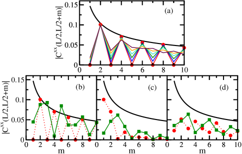
Figure 1: (Color online.) Absolute value of the transverse spin correlation function, $|C^{xx}(L/2,L/2+m)|$ vs $m$ for time $t=10/J$ when only nearest-neighbor couplings are present and for $t=6/J$ when next-nearest-neighbor couplings are also present; $L=20$. For the three models, circle: $\Delta=0$ and square: $\Delta=0.3$. Panels (a) and (b): integrable model with $\epsilon_{L/2+1}=0.0,\alpha=0.0$. In panel (a) the results deviate monotonically from the case where $\Delta=0.0$ as the interaction increases: $\Delta=0.02,0.04,0.06,0.08,0.10$. Panel (c): chaotic model with $\epsilon_{L/2+1}=0.5J,\alpha=0.0$. Panel (d): chaotic model with $\epsilon_{L/2+1}=0.0,\alpha=0.4$.

The results for the chaotic systems are shown in panels (c) and (d). The overall decay of the correlation function is found to be more rapid than for the XX chain [Eq. (10)]. Moreover, both chaotic models show an overall increase in wavelength as $\Delta$ increases. As mentioned before, for the NN+NNN model, the simple correspondence between the nearest-neighbor correlation function ($C^{xx}(n,n+1)$) and current no longer holds. Thus even though the wavelength of oscillations increases for the NN+NNN model as $\Delta$ is increased from $0$ to $0.3$, in this regime the current in fact also increases, as shown in Fig. 2 (c).

III.2 Local spin current

Spin and energy currents, $I_{s}$ and $I_{E}$ respectively, have been extensively studied in the context of integrable periodic chains Zotos et al. (1997); Prelovšek and Zotos ; Zotos and Prelovšek ; Heidrich-Meisner et al. (2003). $I_{E}$ commutes with the Hamiltonian of the XXZ system implying divergent thermal conductivity. Although $I_{s}$ is conserved only for the XX model, it has been argued that spin transport should also be anomalous in the XXZ case when $S^{z}\neq 0$ Zotos et al. (1997); Sirker et al. (2011).

Numerical results for the local spin current, Eqs. (6) and (II.2), for the three models studied here are shown in Fig. 2. For NN couplings only, $I_{s}$ decreases as the strength of the Ising interaction increases for both the integrable model [panel (a)] and the chaotic case with impurity [panel (b)]. For the integrable model, this behavior is expected. Since the energy of the domain wall, $(L-3)\Delta/4$, increases with $\Delta$, the number of states capable of coupling to it decreases and therefore the motion of the excitations becomes more restricted. Equivalently, the eigenstates become spatially more localized. For the system with impurity however, the addition of interaction leads to the onset of chaos and corresponds to eigenstates that are spatially more delocalized. (The relationship between the level of delocalization and the magnitude of the spin current is further explored in Sec. IV). At first sight, the existence of more delocalized eigenstates seems to contradict the decrease of the current, but this decrease may be due to a crossover from ballistic to diffusive transport.

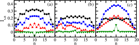
Figure 2: (Color online.) Local current, $I_{s,n}$ [Eqs. (6), (II.2)] vs $n$ for time $t=10/J$ when only nearest-neighbor couplings are present and for $t=6/J$ when next-nearest-neighbor couplings are also present; $L=20$. Panels (a): integrable model with $\epsilon_{L/2+1}=0.0,\alpha=0.0$. Panel (b): chaotic model with $\epsilon_{L/2+1}=0.5J,\alpha=0.0$. Panel (c): chaotic model with $\epsilon_{L/2+1}=0.0,\alpha=0.4$. Circle: $\Delta=0$; square: $\Delta=0.5$; up-triangle: $\Delta=1.0$; down-triangle: $\Delta=2.0$.

The transport behavior of the three models considered here have been studied before. It is ballistic in the integrable domain, which occurs when $\alpha=0,\Delta\leq 1,\epsilon_{n}=0$ Zotos et al. (1997); Heidrich-Meisner et al. (2003); Jung and Rosch (2007) and also when $\alpha=0,\Delta=0,\epsilon_{L/2+1}\neq 0$ Barisic et al. (2009), but it becomes diffusive for the chaotic models. The relationship between non-ballistic transport and the onset of chaos in the single impurity model with interaction was investigated in Ref. Barisic et al. (2009). There it was shown that spin and thermal conductivity relax within a time that scales with the size of the chain. In the case of NNN couplings, the opening of a gap has been associated with diffusive transport Alvarez and Gros (2002b); Heidrich-Meisner et al. (2003, 2004); Langer et al. (2009), but not much work exists that explicitly connects transport behavior with the level of chaoticity of the system.

The model with NNN couplings and $\alpha=0.4$ is chaotic for any value of $\Delta\leq 1$. The results for local current for this system, shown in panel (c), are yet more surprising. Here, the behavior of the current with $\Delta$ is non-monotonic. It first increases with $\Delta$, reaching a maximum level at $\Delta\sim 0.5$, and only then starts diminishing with increasing $\Delta$. The level of spatial delocalization, on the other hand, decreases monotonically with $\Delta$ (see discussion in Sec. IV) and thus cannot justify the result for current. A more thorough analysis of the level of chaoticity in the presence and absence of Ising interaction, as well as how it relates to transport behavior, may shed some light on this scenario.

III.3 Local magnetization

The non-monotonic behavior of the model with $\alpha\neq 0$ is reflected also in the results for the local magnetization in Figs. 3, 4, and 5.

The contour plots in Fig. 3 show the absolute value of the magnetization of each site vs time. The interaction strength increases from top to bottom. For the integrable model (left panels), as $\Delta$ increases, the motion of the excitations becomes more difficult and it takes longer for the sites to reach very low absolute values of the magnetization. A more complicated and asymmetric picture emerges in the presence of an impurity (middle panels), but the trend is still the same. However, when NN and NNN couplings are considered (right panels), as $\Delta$ increases from zero to 0.5, the excitations spread much more efficiently and lead to an enhanced decay of the absolute values of local magnetization. As $\Delta$ is increased beyond $0.5$, the trend finally reverses and the behavior becomes more similar to the other models, where the decay slows down with the Ising interaction.

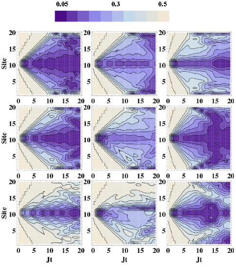
Figure 3: (Color online.) Contour plots of the absolute value of the magnetization of each site $|M_{n}|$ [Eq. (8)] vs time; $L=20$. Left column: integrable model with $\epsilon_{L/2+1}=0.0,\alpha=0.0$. Middle column: chaotic model with $\epsilon_{L/2+1}=0.5J,\alpha=0.0$. Right column: chaotic model with $\epsilon_{L/2+1}=0.0,\alpha=0.4$. Top panels $\Delta=0$; middle panels: $\Delta=0.5$; bottom panels: $\Delta=1.0$. The contour lines range from 0.05 in the darkest region to 0.5 in the lightest region.

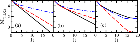
Figure 4: (Color online.) Magnetization of the first half of the chain [Eq. (9)] vs time; $L=20$. Panel (a): integrable model with $\epsilon_{L/2+1}=0.0,\alpha=0.0$. Panel (b): chaotic model with $\epsilon_{L/2+1}=0.5J,\alpha=0.0$. Panel (c): chaotic model with $\epsilon_{L/2+1}=0.0,\alpha=0.4$. Solid line $\Delta=0$; dashed line: $\Delta=0.5$; dot-dashed line: $\Delta=1.0$.

The local magnetization of the first half of the chain [Eq. (9)] is shown in Fig. 4 and reinforces the observations from the contour plots. The decay of $M_{(1,L/2)}$ is linear and the most rapid when $\Delta=0$ in the case of the integrable clean model [panel (a)] and the model with a single impurity [panel (b)]. For these two cases, the decay slows down as the Ising interaction increases. Panel (c), on the other hand, provides a clear illustration of the non-monotonic behavior of the NN+NNN model with $\Delta$. Notice the abrupt and linear decay of $M_{(1,L/2)}$ when $\Delta=0.5$, which is to be contrasted with the slow and nonlinear decay for $\Delta=0$ and 1.

Another perspective to the results of the contour plots is provided in Fig. 5, which shows the behavior of the magnetization $M_{n}$ of site $n$ in time. From this figure one verifies the existence of two different velocities at play. One is related to how fast the magnetization can reach very small values. For the integrable model, $M_{n}$ reaches the lowest values faster when $\Delta$=$0$, which justifies the steep slope of $M_{(1,L/2)}$ (solid line) in Fig. 4 (a), whereas for the chaotic model with NNN couplings, this speed is higher for $\Delta$=$0.5$.

The other velocity is related to the motion of the domain wall front. For the integrable case, this velocity increases with $\Delta$. This is a well known result from Bethe Ansatz Korepin et al. (1993) and bosonization Sirker and Bortz (2006), and has also been studied numerically in Manmana et al. (2009). A rough idea of the front velocity may be obtained by looking at the first moment the magnetization reaches its minimum value. For the integrable model this happens earlier as the Ising interaction increases. Compare, for example, the time when site 10 reaches the lowest magnetization for $\Delta=0$ [top left panel] and $\Delta=1$ [bottom left panel]: it is after $2/J$ for the first and before $2/J$ for the latter. The same pattern is seen for all other sites. By passing an imaginary line through these minima, one sees that the slope becomes steeper as $\Delta$ increases. In the case of the chaotic model with NNN couplings, an evident feature is the suppression of oscillations, but an estimate for the front velocity becomes more difficult. Focusing on the magnetization of the middle site 10, the velocity appears to also show a non-monotonic behavior. Contrary to the integrable case, the front velocity appears to be slightly larger for $\Delta=0$ than for $\Delta=0.5$; it is only for $\Delta>0.5$ that the behavior for the two models become similar and the spin wave velocity increases again with interaction Kol .

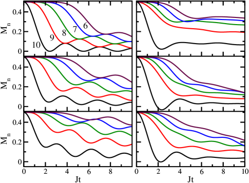
Figure 5: (Color online.) Magnetization of site $n$ vs time; $L=20$. Left panels: integrable clean model with $\epsilon_{L/2+1}=0.0,\alpha=0.0$. Right panels: chaotic clean model with NNN couplings, $\epsilon_{L/2+1}=0.0,\alpha=0.4$. In each panel, the curves range from site 10 to site 6, as indicated in the top left panel. Site 10 corresponds to the center of the domain wall; the up-spin placed here is the first one to move. Top panels $\Delta=0$; middle panels: $\Delta=0.5$; bottom panels: $\Delta=1.0$.

IV Delocalization measure

In an attempt to understand the non-monotonic behavior of the model with NN and NNN couplings, we study here the so-called inverse participation ratio (IPR). For an eigenstate $|\psi_{j}\rangle$ written in the basis vectors $|\phi_{k}\rangle$ as $|\psi_{j}\rangle=\sum_{k=1}^{\text{dim}}c^{k}_{j}|\phi_{k}\rangle$, IPR is defined as

$$\mbox{IPR}_{j}\equiv\frac{1}{\sum_{k=1}^{\text{dim}}|c^{k}_{j}|^{4}}.$$ (12)

This quantity measures the number of basis vectors that contribute to each eigenstate, that is, it measures the level of delocalization of each eigenstate Izrailev (1990); Zelevinsky et al. (1996). It is small when the state is localized and large otherwise. Notice that the result depends on the choice of basis. This choice is made according to the question one is after. In studies of spatial localization, for example, the site-basis is the most appropriate one. When the goal is to separate regular from chaotic behavior, the mean-field basis Zelevinsky et al. (1996), corresponding to the eigenstates of the integrable limit, becomes more relevant.

We consider here the site-basis, since we are interested in quantifying the spatial broadening of the domain wall. For the three models and different values of the Ising interaction strength, Table 1 gives the value of IPR averaged over all eigenstates, $\langle\text{IPR}\rangle$; the number of states that participate in the evolution of the initial domain wall state, $|\Psi(t)\rangle=\sum_{j}C_{j}|\psi_{j}\rangle e^{-iE_{j}t}$, with probability $|C_{j}|^{2}$ larger than $10^{-6}$; and the IPR averaged over these latter eigenstates, $\langle\text{IPR}\rangle_{|C_{j}|^{2}>10^{-6}}$. The purpose of these quantities is the following: $\langle\text{IPR}\rangle$ quantifies the overall level of delocalization of the whole system taking into account all $L!/[(L/2)!]^{2}$ eigenstates; the number of states with $|C_{j}|^{2}>10^{-6}$ identifies the eigenstates that most contribute to the evolution of the domain wall state; and finally $\langle\text{IPR}\rangle_{|C_{j}|^{2}>10^{-6}}$ indicates whether these contributing eigenstates have or have not the same level of delocalization of the whole system.

Table 1: Value of IPR averaged over all eigenstates; number of states participating in the evolution of the domain wall state, $|\Psi(t)\rangle=\sum_{j}C_{j}|\psi_{j}\rangle e^{-iE_{j}t}$, with probability larger than $10^{-6}$; IPR averaged over these eigenstates that contribute with $|C_{j}|^{2}>10^{-6}$. System size: $L=16$, subspace $S^{z}=0$.

Model
($\alpha,\epsilon_{L/2+1}/J$)	$\Delta$	$\langle\text{IPR}\rangle$	$|C_{j}|^{2}$’s $>10^{-6}$	$\langle\text{IPR}\rangle_{|C_{j}|^{2}>10^{-6}}$
(0.0,0.0)	0.0	3075.56	3054	3009.98
(0.0,0.0)	0.5	2358.02	2211	2333.44
(0.0,0.0)	1.0	1732.02	1139	1430.35
(0.0,0.5)	0.0	1921.53	6696	1917.91
(0.0,0.5)	0.5	3679.49	6222	3737.60
(0.0,0.5)	1.0	3118.76	2868	2439.36
(0.4,0.0)	0.0	3906.90	4378	4011.37
(0.4,0.0)	0.5	3684.89	2241	3624.25
(0.4,0.0)	1.0	2840.99	663	1670.35

For the three models, the behavior is the same as $\Delta$ increases from 0.5 to 1.0: the eigenstates become more localized. This is reflected in the dynamics of the three systems: the excitations become more localized, which decreases the magnitude of the spin current and slows down the decay of local magnetization (while the velocity of the domain wall front increases). However, as $\Delta$ changes from 0.0 to 0.5, this correspondence remains valid only for the integrable system, whereas for the other two models orthogonal behaviors are seen:

(i) In the case of the system with impurity, the addition of interaction is followed by a crossover to chaos, which justifies the substantial increase of the value of IPR. The fact that the magnitude of the spin current decreases, going contrary to delocalization, may be indicating a transition from ballistic to diffusive transport, which should slow down the motion of the excitations.

(ii) The system with NN and NNN couplings is chaotic when $\Delta=0.0$ and also when $\Delta=0.5$. Based on the spatial contraction of the eigenstates that occurs when the Ising interaction is turned on, one might expect a decline in the motion of the excitations. However, what is verified in Figs. 2, 3, 4, and 5 is just the opposite. The interpretation of this counter-intuitive behavior requires further studies.

It is interesting to compare the values of $\langle\text{IPR}\rangle$ and $\langle\text{IPR}\rangle_{|C_{j}|^{2}>10^{-6}}$. They are very similar for small $\Delta$, but differ when $\Delta=1$. As mentioned before, the energy of the domain wall increases with the strength of the Ising interaction. At $\Delta=1$ the energy is already very large and close to the edge of the spectrum. In systems with few-body interactions (ours have only two-body interactions), eigenstates with energy close to the edges of the spectrum are more localized Santos and Rigol (2010); Rig . Thus, the eigenstates that contribute to the evolution of the domain wall state are fewer (the numbers in the column of $|C_{j}|^{2}>10^{-6}$ decrease significantly from $\Delta=0.5$ to $\Delta=1.0$) and also more localized than those participating in the evolution of generic initial states ($\langle\text{IPR}\rangle_{|C_{j}|^{2}>10^{-6}}<\langle\text{IPR}\rangle$). This should affect the relaxation process of the domain wall state, which should become slower for large $\Delta$.

V Conclusion

We considered a one-dimensional spin-1/2 system in both integrable and chaotic regimes. The integrable limit corresponded to a clean chain in the presence of nearest-neighbor couplings only. Chaos was induced (i) by adding a single-site impurity field or (ii) by adding next-nearest neighbor couplings. The time-evolution of an initial state in the form of a sharp domain wall was studied.

The analysis of the dynamics focused on transverse spin correlation function, local spin current, and local magnetization. In order to understand the behavior of these quantities, we resorted to delocalization measures; the motivation being that usually a good picture of the static properties of a system may indicate what to expect for its time evolution. This approach served us well when dealing with the integrable model. Here, as the Ising interaction strength $\Delta$ increases, the level of spatial delocalization of the eigenstates lowers and, as one might expect, the magnitude of the spin current decreases and the decay of the absolute value of local magnetization slows down.

The same behavior was verified for the chaotic models for the case of large $\Delta$, but for small Ising interaction, the level of delocalization changed in a way contrary to the change in current and magnetization. For model (i), the addition of interaction leads to the onset of chaos and consequently the eigenstates further delocalize. The magnitude of the current, however, decreased. We speculate that this is due to the transition from ballistic to diffusive transport. For model (ii), the system is already chaotic at $\Delta=0$ and the eigenstates only shrink with the Ising interaction. Contrary to that, the motion of the excitations is enhanced, as attested by the results for spin current and local magnetization. Further studies are needed to clarify this behavior.