Dynamics of diffusion controlled chain closure: flexible chain in presence of hydrodynamic interaction

Abstract

Based on the Wilemski-Fixman approach (J. Chem. Phys. 60, 866 (1974)) we showed that for a flexible chain in $\theta$ solvent hydrodynamic interaction treated with an pre-averaging approximation makes ring closing faster if the chain is not very short. Only for a very short chain the ring closing is slower with hydrodynamic interaction on. We have also shown that the ring closing time for a chain with hydrodynamic interaction in $\theta$ solvent scales with the chain length ($N$) as $N^{1.527}$, in good agreement with previous renormalization group calculation based prediction by Freidman et al. (Phys. Rev. A. 40, 5950 (1989)).

I introduction

Dynamics of loop formation in long chain molecules has been a subject of immense interest to experimentalists Winnik (1986); Haung et al. (2010); Lapidus et al. (2002); Hudgins et al. (2002) and theoreticians Wilemski and Fixman (1974); Doi (1975); Perico and Cuniberti (1977); Szabo et al. (1980); Pastor et al. (1996); Srinivas et al. (2002); Dua and Cherayil (2002a, b); Debnath and Cherayil (2004); Portman (2003); Sokolov (2003); Toan et al. (2008); Santo and Sebastian (2009) for over a decade. Recently the dynamics of loop formation has found greater importance because of its relevance in biophysics. Advances in single molecule techniques made it possible to monitor the kinetics of loop formation involving biomolecules at the single molecule level Cloutier and Widom (2005); Thirumalai and Hyeon (2005). Loop formation is a prime step in protein Buscaqlia et al. (2005) and RNA folding Thirumalai et al. (2001). Also a measure of the intrinsic flexibility of DNA can be found from the rate at which it undergoes cyclization Cloutier and Widom (2005).

Loop formation in polymers is essentially a many body problem as a polymer is made of many connected segments and hence an exact analytical solution is impossible. All the theories of loop closing dynamics are approximate Wilemski and Fixman (1974); Szabo et al. (1980). Although many theoretical and simulation attempts have been made to investigate the effect of flexibility Santo and Sebastian (2009), solvent quality Debnath and Cherayil (2004) on the loop closing dynamics, not much theoretical investigation has been performed to shed light on the effects of hydrodynamic interaction on loop closing dynamics other than the renormalization group calculation by Freidman et al Friedman and O’Shaughnessy (1989). Hydrodynamic interaction which is essentially nonlocal in space has been shown to have profound effects on the dynamics of long chain molecules Das et al. (2010); Iznitli et al. (2008). The rate of translocation of polymer through a nano-pore has been shown to be greatly affected in presence of hydrodynamic interaction Iznitli et al. (2008); Ali and Yeomans (2005). Recently it has been theoretically shown Das et al. (2010) that the breakage rate of stretched polymer tethered to soft bond get enhanced in presence of hydrodynamic interaction.

In this paper we investigate the effect of hydrodynamic interaction on the ring closing dynamics of a flexible chain in $\theta$ solvent. It is well known that the ring closing time ($\tau$) for a flexible chain without excluded volume and hydrodynamic interaction (Rouse chain Doi and Edwards (1988)) scales with the chain length ($N$) as $N^{2}$ in the Wilemski-Fixman (WF) Wilemski and Fixman (1974) theoretical framework. Here we use Zimm model Doi and Edwards (1988) for the polymer which actually takes care of the hydrodynamic interaction at the simplest possible level. Our calculation shows that hydrodynamic interaction profoundly affect the rate of loop formation and also has a different scaling relation with the length of the polymer $N$. The rest of the paper is arranged as follows. In Sec. II the Wilmeski-Fixman (WF) theory for the chain closure Wilemski and Fixman (1974) is briefly discussed. WF formalism gives a prescription to calculate the ring closing time as an integral over a sink-sink time correlation function. Sec. III deals with a brief description of the radial delta function sink which is used later in the calculation of the ring closing time. Time correlation formalism for the flexible chain with and without hydrodynamic interaction is discussed in Sec. IV. Sec. V presents the results and VI is devoted to conclusions.

II Theory of Chain Closure

In an stochastic environment the dynamics of a single polymer chain having reactive end-groups is modeled by the following Smoluchowski equation in WF theory Wilemski and Fixman (1974).

$$\frac{\partial P(\{\mathbf{R}\},t)}{\partial t}=LP(\{\mathbf{R}\},t)-kS(\{\mathbf{R}\})P(\{\mathbf{R}\},t)$$ (1)

Here $P(\{R\},t)$ is the distribution function for the chain that it has the conformation $\{R\}\equiv R_{1},$$R_{2},$$......R_{n}$ at time $t$ where $R_{i}$ denotes the position of the $i$th monomer in the chain of $n$ monomers. $S({R})$ is called the sink function which actually models the reaction between the ends and thus usually is a function of end to end vector. $L$ is a differential operator, defined as

$$L=D_{0}\sum_{i=1}^{n}\frac{\partial}{\partial\mathbf{R}_{i}}.\left[\frac{\partial}{\partial\mathbf{R}_{i}}+\frac{\partial U}{\partial\mathbf{R}_{i}}\right]P(\{\mathbf{R}\},t)$$ (2)

Here $D_{0}$ is the diffusion coefficient of the chain defines as the inverse of the friction coefficient per unit length and $U$ is the potential energy of the chain. Wilemski and Fixman then derived an approximate expression for the mean first passage time from Eq. (1). This mean first passage time is actually the loop closing time for the chain. The expression for this loop closing time reads

$$\tau=\int_{0}^{\infty}dt\left(\frac{C(t)}{C(\infty)}-1\right)$$ (3)

Where $C(t)$ is the sink-sink correlation function defined as

$$C(t)=\int d\mathbf{R}\int d\mathbf{R}_{0}S(\mathbf{R})G(\mathbf{R},t|\mathbf{R}_{0},0)S(\mathbf{R}_{0})P(\mathbf{R}_{0})$$ (4)

In the above expression $G(\mathbf{R},t|\mathbf{R}_{0},0)$ is the Greens function or the conditional probability that a chain with end-to-end distance $R_{0}$ at time $t=0$ has the end-to-end distance $R$ at time $t$; $P(R_{0})$ is the equilibrium distribution of the end to end distance since the chain was in equilibrium at time $t=0$. $S(R)$ is the sink function Sebastian (1992); Debnath et al. (2006); Chakrabarti (2010) which depends only on the separation between the chain ends. We would like to comment that Eq. (3) is not exact and only valid in the limit of infinite sink strength, $k\to\infty$ as this closing time is nothing but the mean first passage time Redner (2001); Chakrabarti and Sebastian (2009).

Now it is obvious that the knowledge of the Greens function, $G(\mathbf{R},t|\mathbf{R}_{0},0)$ is prerequisite to calculate the sink-sink correlation function $C(t)$ and hence the closing time $\tau$. In case of a flexible chain the Greens function and the end-to-end probability distribution functions are known and Gaussian.

For a flexible chain the Greens function is given by

$$G(\mathbf{R},t|\mathbf{R}_{0},0)=\left(\frac{3}{2\pi\left\langle R^{2}\right\rangle_{eq}}\right)^{3/2}\frac{1}{\left(1-\phi^{2}(t)\right)^{3/2}}\times\exp\left[-\frac{3(\mathbf{R}-\phi(t)\mathbf{R}_{0})^{2}}{2\left\langle R^{2}\right\rangle_{eq}(1-\phi^{2}(t))}\right]$$ (5)

Where

$$\phi(t)=\frac{\left\langle\mathbf{R}(t).\mathbf{R}(0)\right\rangle_{eq}}{\left\langle R^{2}\right\rangle_{eq}}$$ (6)

is the normalized end-to-end vector correlation function for the chain. The above ensemble average is taken over the initial equilibrium distribution for end-to-end vector $P(\mathbf{R}_{0})$.

Similarly end-to-end equilibrium distribution for the flexible chain at time $t=0$ is given by Doi and Edwards (1988); Sokolov (2003)

$$P(R_{0})=\left(\frac{3}{2\pi L^{2}}\right)^{3/2}\exp\left[-\frac{3R_{0}^{2}}{2L^{2}}\right]$$ (7)

With the above Gaussian functions the sink-sink correlation function can be written as a radial double integral.

$$C(t) = \left(\frac{3}{2\pi L^{2}}\right)^{3}\frac{1}{\left(1-\phi^{2}(t)\right)^{3/2}}\int_{0}^{\infty}4\pi R^{2}S(R)dR\int_{0}^{\infty}4\pi R_{0}^{2}S(R_{0})dR_{0}\times$$ (8)

$$\exp\left[-\frac{3}{2L^{2}}\frac{(R^{2}+R_{0}^{2})}{(1-\phi^{2}(t))}\right]\frac{\sinh\left[(3\phi(t)RR_{0})/(L^{2}(1-\phi^{2}(t)))\right]}{(3\phi(t)RR_{0})/(L^{2}(1-\phi^{2}(t)))}$$

The above integral can be evaluated analytically for some specific choice of the sink functions. With a radial delta function sink the above integral can be evaluated analytically.

III The radial delta function sink

For our case study we choose a radial delta function sink Pastor et al. (1996), $S(R)=\delta(R-a)$. Since in this case the integration over $R$ and $R_{0}$ can be carried out analytically, the looping time can be expressed in a closed form as follows.

$$\tau=\int_{0}^{\infty}dt\left(\frac{\exp\left[-(2x_{0}\phi^{2}(t))/(1-\phi^{2}(t))\right]\sinh\left[(2x_{0}\phi(t))/(1-\phi^{2}(t))\right]}{2x_{0}\phi(t)\sqrt{1-\phi^{2}(t)}}-1\right)$$ (9)

with

$$x_{0}=\frac{3a^{2}}{2L^{2}}$$

Obviously if the end-to-end vector correlation function $\phi(t)$ is known the closing time can be calculated by carrying out the integration over time. Here we calculate the looping time given by the above expression for a flexible polymer in presence and absence of hydrodynamic interaction and make a comparative study. Throughout the paper it is assumed that the chain was in equilibrium at $t=0$ and only at $t=0^{+}$ the hydrodynamic interaction is turned on (for the Zimm chain). Thus the equilibrium end-to-end distribution for the Rouse as well as for the Zimm chain is given by (Eq.(7)). The last integration over time is not analytical so has to be carried out numerically.

IV Flexible polymer without and with hydrodynamic interactions

The simplest dynamical description of a flexible chain or polymer in solution is given by Rouse Model Doi and Edwards (1988); Kawakatsu (2004). This model does not take into account of excluded volume and hydrodynamic interaction and has been the basis of dynamics of dilute polymer solution and has been successfully used in the context of ring closing in polymers Srinivas et al. (2002), breathing dynamics in DNA Chakrabarti (2011), polymer translocation Sebastian and Paul (2000) etc. In the continuum limit the governing equation of motion for the position vector $\mathbf{R}(n,t)$ is given by

$$\zeta\frac{\partial\mathbf{R}(n,t)}{\partial t}=k\frac{\partial^{2}\mathbf{R}(n,t)}{\partial n^{2}}+f(n,t)$$ (10)

Here $n$ is a continuous variable, $k=\frac{3k_{B}T}{b^{2}}$ where $b$ is the length of a monomer in the discrete representation of the Rouse polymer and $f(n,t)$ is the random force with the moments

$$\left\langle f(n,t)\right\rangle = 0$$

$$\left\langle f_{\alpha}(n,t_{1})f_{\beta}(m,t_{2})\right\rangle = 2\zeta k_{B}T\delta(n-m)\delta_{\alpha\beta}\delta(t_{1}-t_{2})$$ (11)

It is straightforward to show that the Rouse normal modes ($X_{p}$) obey the following equation

$$\zeta_{p}\frac{\partial{X}_{p}}{\partial t}=-k_{p}X_{p}+f_{p}(t)$$ (12)

Where $\zeta_{0}=N\zeta$, $\zeta_{p}=2N\zeta$ for $p=0,1,2,...$ and $k_{p}=2\pi^{2}kp^{2}/N=\frac{6\pi^{2}k_{B}T}{Nb^{2}}p^{2}$ for $p=0,1,2,...$. Here $f_{p}(t)$ is the random force satisfying $\left<f_{p\alpha}\right>=0$ and $\left<f_{p\alpha}(t)f_{q\beta}(t_{1})\right>=2\delta_{pq}\delta_{\alpha\beta}\zeta_{p}k_{B}T\delta(t-t_{1})$.

Then for a Rouse polymer it can be shown that the normalized end-to-end vector time correlation function defined in (6) is given by

$$\phi(t)=\frac{\left\langle\mathbf{R}(t).\mathbf{R}(0)\right\rangle_{eq}}{\left\langle R^{2}\right\rangle_{eq}}=\sum_{p=odd}\frac{8}{p^{2}\pi^{2}}e^{-tp^{2}/\tau_{1}}=\sum_{p=odd}\frac{8}{p^{2}\pi^{2}}e^{-t\omega^{Rouse}_{p}}$$ (13)

Where $\tau_{1}=\frac{\zeta N^{2}b^{2}}{3\pi^{2}k_{B}T}$ and $\omega^{Rouse}_{p}=\frac{p^{2}}{\tau_{1}}$.

The simplest possible model for the dynamics of a flexible chain with the hydrodynamic interaction but without the excluded volume interaction is known as the Zimm model Doi and Edwards (1988); Kawakatsu (2004). In $\theta$ condition the continuum limit equation of motion for the position vector $\mathbf{R}(n,t)$ in the Zimm model is given by

$$\zeta\frac{\partial\mathbf{R}(n,t)}{\partial t}=\sum_{m}H_{mn}.\left(k\frac{\partial^{2}\mathbf{R}(m,t)}{\partial m^{2}}+f(m,t)\right)$$ (14)

Here $H_{mn}$ is the mobility matrix and is generally a nonlinear function of $\mathbf{R}(n,t)-\mathbf{R}(m,t)$ and the above equation is quite difficult to handle. To simplify this analysis Zimm introduced a pre-averaging approximation, which replaces $H_{mn}$ by its equilibrium average, $\left\langle H_{mn}\right\rangle_{eq}$.  It can be shown that with this pre-averaging approximation Doi and Edwards (1988) becomes a linear function of $\mathbf{R}(n,t)$.

$$\zeta\frac{\partial\mathbf{R}(n,t)}{\partial t}=\sum_{m}h(n-m)\left(k\frac{\partial^{2}\mathbf{R}(m,t)}{\partial m^{2}}+f(m,t)\right)$$ (15)

where $h(n-m)$ decreases slowly as $h(n-m)\propto\left|(n-m)\right|^{-1/2}$. Thus in Zimm model interaction among the segments is not localized. This is how a Zimm chain in different from a Rouse chain.

It is possible to show Doi and Edwards (1988) that for the Zimm chain in $\theta$ solvent, the normal modes ($X^{Zimm,\theta}_{p}$) can be shown to obey an equation which has the same structure as the Rouse normal modes

$$\zeta_{p}\frac{\partial{X}^{Zimm,\theta}_{p}}{\partial t}=-k_{p}{X}^{Zimm,\theta}_{p}+f_{p}(t)$$ (16)

Where $\zeta_{p}=\zeta\sqrt{\frac{\pi Np}{3}}$ for $p=0,1,2,...$ and $k_{p}=2\pi^{2}kp^{2}/N=\frac{6\pi^{2}k_{B}T}{Nb^{2}}p^{2}$ for $p=0,1,2,...$. Here $f_{p}(t)$ is the random force satisfying $\left<f_{p\alpha}\right>=0$ and $\left<f_{p\alpha}(t)f_{q\beta}(t_{1})\right>=2\delta_{pq}\delta_{\alpha\beta}\zeta_{p}k_{B}T\delta(t-t_{1})$.

In case of $\theta$ solvent condition the normalized end-to end vector time correlation function (Eq.(6)) for the Zimm chain is given by

$$\phi(t)=\frac{\left\langle\mathbf{R}(t).\mathbf{R}(0)\right\rangle_{eq}}{\left\langle R^{2}\right\rangle_{eq}}=\sum_{p=odd}\frac{8}{p^{2}\pi^{2}}e^{-tp^{3/2}/\tau^{Zimm,\theta}_{1}}=\sum_{p=odd}\frac{8}{p^{2}\pi^{2}}e^{-t\omega^{Zimm,\theta}_{p}}$$ (17)

Where $\tau^{Zimm,\theta}_{1}=\frac{\zeta N^{3/2}b^{2}}{6\sqrt{3}\pi^{3/2}k_{B}T}$ and $\omega^{Zimm,\theta}_{p}=\frac{p^{3/2}}{\tau^{Zimm,\theta}_{1}}$.

In principle it is straightforward to calculate the closing time with a delta function sink (Eq.(9)) as it involves evaluating $\phi(t)$ and carrying out an integration over time. We evaluate $\phi(t)$ for both the cases exactly by carrying out the sums defined in (Eq.(13)) and (Eq.(17)).

Figure 1: $\phi(t)$ against time ($t$). The values of other parameters used are: $N=1,b=1,\zeta=1,k_{B}T=1$. In the inset the short time ($t$) behavior of $\tau$ is shown. Note up to a short time range $\phi(t)$ for the chain with hydrodynamic interaction (Zimm chain in $\theta$ solvent) decays slowly as compared to a chain without hydrodynamic interaction (Rouse chain).

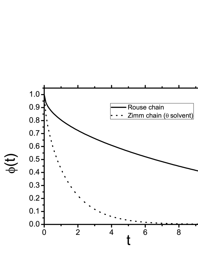
Figure 2: $\phi(t)$ against time ($t$). The values of other parameters used are: $N=20,b=1,\zeta=1,k_{B}T=1$.

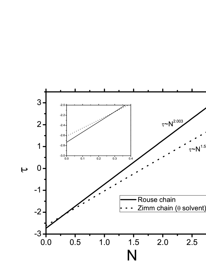
Figure 3: $\tau$ against the chain length($N$). The values of other parameters used are: $b=1,\zeta=1,k_{B}T=1,a=0.01$. In the inset $\tau$ for a short range of the chain length, $N$ shown. Note for a very short chain the $\tau$ for the chain with hydrodynamic interaction (Zimm chain in $\theta$ solvent) is higher meaning a slower ring closure.

V Results

The closing time ($\tau$) with the radial delta function sink is calculated for the Rouse chain as well as for the Zimm chain in $\theta$ solvent. Calculation of $\tau$ involves evaluating $\phi(t)$ for the respective chains and then putting it in Eq. (9) followed by an integration over time which has to be carried out numerically. The end-to-end vector correlation function defined in Eq. (6) is actually a sum over the decays of all the odd modes and at a given time $t$ the bulk of the contribution to $\phi(t)$ comes from the lower normal modes. Each normal mode decays with an effective rate constant, $\omega^{Rouse}_{p}=p^{2}/\tau_{1}$ for the Rouse chain (Eq.(13)) and in case of a Zimm chain in $\theta$ solvent it is $\omega^{Zimm,\theta}_{p}=p^{3/2}/\tau^{Zimm,\theta}_{1}$ (Eq.(17)). Now had it been $\tau_{1}=\tau^{Zimm,\theta}_{1}$ all the odd modes of the Rouse chain hence the end-to-end vector correlation function would have decayed faster resulting a faster ring closure compared to that for a Zimm chain in $\theta$ solvent. In reality $\tau_{1}\neq\tau^{Zimm,\theta}_{1}$ and the ratio $\omega^{Zimm,\theta}_{p}/\omega^{Rouse}_{p}$ has a strong length ($N$) dependence, $\omega^{Zimm,\theta}_{p}/\omega^{Rouse}_{p}=\frac{(\tau_{1}/\tau^{Zimm,\theta}_{1})}{\sqrt{p}}=\frac{2\sqrt{3}}{\sqrt{\pi}}\sqrt{N/p}$. Only when, $\sqrt{N/p}<<\frac{2\sqrt{3}}{\sqrt{\pi}}$ the normal modes of the Zimm chain in $\theta$ solvent decay faster. For a very short chain or in case of higher normal modes the condition $\sqrt{N/p}<<\frac{2\sqrt{3}}{\sqrt{\pi}}$ can be achieved and then only the normal modes for the Zimm chain (in $\theta$ solvent) will decay slowly compared to the normal modes of the Rouse chain. Thus for a short Zimm chain (in $\theta$ solvent) initial decay of $\phi(t)$ is slow compared to a Rouse chain. This is shown in the inset of Fig. 1. On the other hand for a long Zimm chain all the normal modes decay faster than the Rouse chain normal modes. This naturally results a slowly decaying $\phi(t)$ for a Rouse chain as is shown in Fig. 2.

In Fig. 3 log-log plot of the closing time ($\tau$) is plotted against the chain length $N$ for both the chains. The slope for the Rouse chain has been found out to be $2.003$ very close to previously found values based on WF theory calculation Debnath and Cherayil (2004); Thirumalai and Hyeon (2005). For the Zimm chain (in $\theta$ solvent) the slope is $1.527$. Thus hydrodynamic interaction makes ring closure faster. Also notice for a very short chain the ring closure is faster for a Rouse chain as shown in the inset of Fig. 3. This actually suggests that the proportionality factor or the frequency factor between the ring closing rate, $\tau$ and $N^{\alpha}$, where $\alpha=1.527$ with the hydrodynamic interaction on and $\alpha=2.003$ without the hydrodynamic interaction, too has a length ($N$) dependence.

VI Conclusions

In this paper we show that the hydrodynamic interaction makes ring closure faster within WF Wilemski and Fixman (1974) framework if the chain is not very short. For a very short chain ring closure can be slower in presence of hydrodynamic interaction. The ring closing time ($\tau$) for the Zimm chain (in $\theta$ solvent) scales as $N^{1.527}$. This is actually in very good agreement with the renormalization group calculation prediction of Friedman et al. Friedman and O’Shaughnessy (1989). They showed that for a Zimm chain not too short the closing time scales as $N^{3/2}$. But surprisingly $N^{3/2}$ behavior can also be seen even without hydrodynamic interaction. For example, harmonic chain approximation within WF framework leads to similar scaling Doi (1975). Also in the model of Szabo, Schulten and Schulten (SSS) Szabo et al. (1980), in which the difficult problem of the polymeric chain having many degrees of freedom is replaced with a single particle diffusing in a potential of mean force predicts $N^{3/2}$ scaling for a chain without hydrodynamic interaction. Portman Portman (2003) pointed out that SSS theory Szabo et al. (1980) actually gives a lower bound to the chain closing time and WF theory Wilemski and Fixman (1974) gives an upper bound. So a faster ring closure in SSS formalism as compared to WF theory prediction is expected. Experimentally the closure rate $\kappa$ for a $10-20$ residue polypeptides of the alanine-gylcine-glutamine trimer have been found out to be vary as $N^{-3/2}$ for large $N$ Lapidus et al. (2002). Although in accordance with SSS theory Szabo et al. (1980), this faster ring closing as compared to a flexible chain without hydrodynamic interaction might also be due to hydrodynamic interaction as found in our theoretical analysis here.

Thus just by looking at the length dependence of the ring closing time it is rather impossible to comment on the microscopic basis of ring closure. Similar scalings can arise due to completely different reasons. As a future problem it will be interesting to see what happens to the closing time for a chain with hydrodynamic interaction as different sink functions are used and also in the SSS formalism Szabo et al. (1980). It is expected since the SSS formalism gives a lower bound to the ring closing rate Portman (2003), ring closing with the hydrodynamic interaction work in the SSS framework will make ring closing even faster as compared to in the WF framework.

VII acknowledgement

This work was supported by the Department of Science and Technology through the J. C. Bose fellowship project of K. L. Sebastian. The author thanks K. L. Sebastian for illuminating discussions.

References

- Winnik (1986) M. A. Winnik, In Cyclic Polymers, Chapter 9 (Elsivier, New York, 1986).
- Haung et al. (2010) Z. Haung, H. Ji, J. Mays, and M. Dadmun, Langmuir 26, 202 (2010).
- Lapidus et al. (2002) L. J. Lapidus, P. J. Steinbach, W. A. Eaton, A. Szabo, and J. Hofrichter, J. Phys. Chem. B 106, 11628 (2002).
- Hudgins et al. (2002) R. R. Hudgins, F. Huang, G. Gramlich, and W. M. Nau, J. Am. Chem. Soc. 124, 556 (2002).
- Wilemski and Fixman (1974) G. Wilemski and M. Fixman, J. Chem. Phys. 60, 866 (1974).
- Doi (1975) M. Doi, Chem. Phys. 9, 455 (1975).
- Perico and Cuniberti (1977) A. Perico and C. Cuniberti, J. Polym. Sci.,Polym. Phys. Ed. 15, 1435 (1977).
- Szabo et al. (1980) A. Szabo, K. Schulten, and Z. Schulten, J. Chem. Phys. 72, 4350 (1980).
- Pastor et al. (1996) R. W. Pastor, R. Zwanzig, and A. Szabo, J. Chem. Phys. 105, 3878 (1996).
- Srinivas et al. (2002) G. Srinivas, B. Bagchi, and K. L. Sebastian, J. Chem. Phys. 116, 7276 (2002).
- Dua and Cherayil (2002a) A. Dua and B. J. Cherayil, J. Chem. Phys. 116, 399 (2002a).
- Dua and Cherayil (2002b) A. Dua and B. J. Cherayil, J. Chem. Phys. 117, 7765 (2002b).
- Debnath and Cherayil (2004) P. Debnath and B. J. Cherayil, J. Chem. Phys. 120, 2482 (2004).
- Portman (2003) J. J. Portman, J. Chem. Phys. 118, 2381 (2003).
- Sokolov (2003) I. M. Sokolov, Phys. Rev. Lett. 90, 080601 (2003).
- Toan et al. (2008) N. M. Toan, G. Morrison, C. Hyeon, and D. Thirumalai, J. Phys. Chem. B 112, 6094 (2008).
- Santo and Sebastian (2009) K. P. Santo and K. L. Sebastian, Phys. Rev. E. 80, 061801 (2009).
- Cloutier and Widom (2005) T. E. Cloutier and J. Widom, Proc. Natl. Acad. Sci. U.S.A. 102, 5397 (2005).
- Thirumalai and Hyeon (2005) D. Thirumalai and C. Hyeon, Biochemistry 44, 4957 (2005).
- Buscaqlia et al. (2005) M. Buscaqlia, J. Kubelka, W. A. Eaton, and J. Hofrichtev, J. Mol. Biol. 347, 657 (2005).
- Thirumalai et al. (2001) D. Thirumalai, N. Lee, S. A. Woodson, and D. Klimov, Annu. Rev. Phys. Chem. 52, 751 (2001).
- Friedman and O’Shaughnessy (1989) B. Friedman and B. O’Shaughnessy, Phys. Rev. A 40, 5950 (1989).
- Das et al. (2010) S. G. Das, D. Pescia, M. Biswas, and A. Sain, Phys. Rev. E. 82, 041910 (2010).
- Iznitli et al. (2008) A. Iznitli, D. C. Schwartz, M. D. Graham, and J. J. de Pablo, J. Chem. Phys. 128, 085102 (2008).
- Ali and Yeomans (2005) I. Ali and J. M. Yeomans, J. Chem. Phys. 123, 234903 (2005).
- Doi and Edwards (1988) M. Doi and S. F. Edwards, The Theory of Polymer Dynamics (Clarendon Press. Oxford, 1988).
- Sebastian (1992) K. L. Sebastian, Phys. Rev. A. 46, R1732 (1992).
- Debnath et al. (2006) A. Debnath, R. Chakrabarti, and K. L. Sebastian, J. Chem. Phys. 124, 204111 (2006).
- Chakrabarti (2010) R. Chakrabarti, Chem. Phys. Lett. 495, 60 (2010).
- Redner (2001) S. Redner, A Guide to First Passage Processes (Cambridge University Press, Cambridge UK, 2001).
- Chakrabarti and Sebastian (2009) R. Chakrabarti and K. L. Sebastian, J. Chem. Phys. 131, 224504 (2009).
- Kawakatsu (2004) T. Kawakatsu, Statistical Physics of Polymers An Introduction (Springer, 2004).
- Chakrabarti (2011) R. Chakrabarti, Chem. Phys. Lett. 502, 107 (2011).
- Sebastian and Paul (2000) K. L. Sebastian and A. K. R. Paul, Phys. Rev. E. 62, 927 (2000).