Exact Entanglement Dynamics Beyond the Rotating Wave Approximation

Abstract

The entanglement dynamics of two remote qubits is examined analytically. The qubits interact arbitrarily strongly with separate harmonic oscillators in the idealized degenerate limit of the Jaynes-Cummings Hamiltonian. In contrast to well known non-degenerate RWA results, it is shown that ideally degenerate qubits cannot induce bipartite entanglement between their partner oscillators.

I Introduction

Entanglement is considered a necessary resource for many of the algorithms proposed for quantum computation and communication Nielsen and Chuang (2000). Over the course of the last decade there has been a growing interest in finding ways to quantify Horodecki et al. (2009), manipulate, and control Raimond et al. (2001) the initial entanglement shared by different parties when they come in contact with different local Benatti, Floreanini, and Piani (2003); *PhysRevLett.89.277901; *PhysRevA.65.040101; *PhysRevA.68.062316; *springerlink:10.1007/s11128-009-0137-6; *springerlink:10.1134/S0030400X10030069 and non-local Yu and Eberly (2004); Yönaç et al. (2006); Bellomo et al. (2007); Al-Qasimi and James (2008); Chruściński and Kossakowski (2010); Liu and Goan (2007) environments. For two remote systems coming in contact with two uncorrelated reservoirs, typically the initial entanglement between the two systems ultimately ends up as a bipartite entanglement between the two reservoirs López et al. (2008). For the single mode environments, however, the entanglement dynamics depends strongly on the initial state of the two environments and the interaction between each system and the corresponding environment Yönaç et al. (2006); Yönaç and Eberly (2010).

In many of the previous investigations the Jaynes-Cummings (JC) model Jaynes and Cummings (1963) has been invoked to describe the interaction between each party, described as qubits, and the corresponding environment, modeled by a harmonic oscillator. The JC Hamiltonian reads

$$H=\hbar\frac{\omega_{0}}{2}\sigma_{z}+\hbar\omega a^{\dagger}a+\hbar\lambda(a^{\dagger}+a)\sigma_{x},$$ (1)

where $\sigma_{z}$ and $\sigma_{x}$ are Pauli matrices and $a$ and $a^{\dagger}$ are the usual ladder operators. The model has been used extensively to describe the interaction between an atom and a single mode of a cavity in quantum optics Jaynes and Cummings (1963); Allen and Eberly (1987). In the studies of strong light-matter interaction and/or in the search for potential quantum computation and quantum information applications, the model has also been invoked to describe the interaction between a Cooper pair box with a nanomechanical resonator Irish and Schwab (2003) or with a transmission line resonator Blais et al. (2004); Wallraff et al. (2004), etc. In quantum optics, typically, the nearly resonant ($|\omega-\omega_{0}|\ll\omega+\omega_{0}$) and weak coupling ($\lambda\ll\omega,\omega_{0})$ conditions apply and the rotating wave approximation (RWA) is valid Jaynes and Cummings (1963); Allen and Eberly (1987). Yet with the advent of circuit QED it has become feasible experimentally to explore regimes of the model where the dynamics is not well described within the RWA Niemczyk et al. (2010); Fedorov et al. (2010); Forn-Díaz et al. (2010).

There have already been many investigations exploring analytically and/or numerically the local dynamics of the model beyond the RWA *[][andreferencestherein]BWShorebook; Swain (1973); *PhysRevA.46.4138; *PhysRevA.68.063811; *1402-4896-76-2-007; Zaheer and Zubairy (1988); Finney and Gea-Banacloche (1994); Irish (2007); Irish et al. (2005); Casanova et al. (2010); Hausinger and Grifoni (2010) . Some of the developed techniques deal with nearly resonant but strong couplings Irish (2007); Finney and Gea-Banacloche (1994); Zaheer and Zubairy (1988) and some deal with highly detuned and/or strong coupling scenarios Irish et al. (2005); Casanova et al. (2010); Hausinger and Grifoni (2010). Remote entanglement dynamics beyond the RWA has also been the subject of a recent note by Chen et al. Chen et al. (2010). They focused on the nearly resonant and strong coupling scenario. In this note we present exact analytic formulas for the entanglement dynamics, beyond the RWA, in the far from resonance regime of the model where the qubits are degenerate $(\omega_{0}=0)$. A study of the dynamics of a degenerate qubit interacting with a classical field, and a discussion of a physical system which can be treated as a degenerate qubit, has been given by Shakov and McGuire Shakov and McGuire (2003).

In Fig. 1 we present a schematic comparison of the energy levels of the qubit and the harmonic oscillator in both RWA and near-degenerate regimes. The system we study consists of two non-communicating subsystems. Each subsystem itself consists of a qubit that interacts with a partner harmonic oscillator. From now on we refer to the harmonic oscillators as the fields.

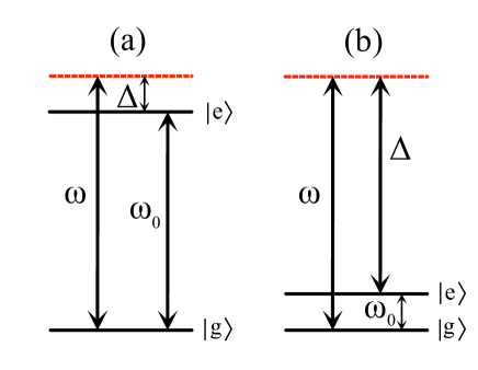
Figure 1: The energy level representation of (a) RWA and (b) nearly degenerate regime. In the degenerate regime $\omega_{0}=0$.

The structure of the current note is as follows. In section II we briefly examine the JC Hamiltonian in the degenerate regime. Section III is devoted to the dynamics of a single qubit and a single harmonic oscillator in the degenerate regime where we completely avoid the RWA. In section IV we focus on a certain class of initial states to study the entanglement dynamics of two remote initially entangled qubits in the degenerate regime. The effect of different initial fields as well as the effect of coupling strength on the bipartite entanglement in the degenerate regime is studied. Intuitively we may think that when two separable fields come in contact with remote entangled qubits, some of the coherence between the two qubits gets transferred to the fields and they develop bipartite entanglement Yönaç et al. (2007). We show that in the degenerate regime two initially separable fields do not develop bipartite entanglement.

II Degenerate Regime

In the degenerate regime $(\omega_{0}=0)$, the JC Hamiltonian reads

$$H =\left(\hbar\omega a^{\dagger}a+\hbar\lambda(a^{\dagger}+a)+\hbar\frac{\lambda^{2}}{\omega}\right)|\uparrow\rangle\langle\uparrow|$$ (2)

$$+\left(\hbar\omega a^{\dagger}a-\hbar\lambda(a^{\dagger}+a)+\hbar\frac{\lambda^{2}}{\omega}\right)|\downarrow\rangle\langle\downarrow|.$$

In this note $\sigma_{x}|\uparrow\rangle=|\uparrow\rangle$, $\sigma_{x}|\downarrow\rangle=-|\downarrow\rangle$, $\sigma_{z}|e\rangle=|e\rangle$ and $\sigma_{z}|g\rangle=-|g\rangle$. For simplicity we added a constant value ($\hbar\frac{\lambda^{2}}{\omega}$) to the Hamiltonian that has no effect on the dynamics. $H$ can be diagonalized as follows:

$$H|E_{n,\pm}\rangle=E_{n}|E_{n,\pm}\rangle,~{}~{}~{}~{}~{}~{}~{}~{}E_{n}=n\hbar\omega,$$

$$|E_{n,+}\rangle=|\uparrow,n_{+}\rangle,$$

$$|n_{+}\rangle=D^{\dagger}(\beta)|n\rangle=D^{\dagger}(\beta)\frac{{a^{\dagger}}^{n}}{\sqrt{n!}}|0\rangle,$$

$$|E_{n,-}\rangle=|\downarrow,n_{-}\rangle,$$

$$|n_{-}\rangle=D^{\dagger}(-\beta)|n\rangle=D^{\dagger}(-\beta)\frac{{a^{\dagger}}^{n}}{\sqrt{n!}}|0\rangle.$$ (3)

Here $\beta=\frac{\lambda}{\omega}$, and $D(\beta)=\exp(\beta a^{\dagger}-\beta^{*}a)$ is the harmonic oscillator displacement operator. The set of all eigenstates provides a complete basis for the Hilbert space and the closure relation reads

$$\sum_{n}\Big{(}|\uparrow,n_{+}\rangle\langle\uparrow,n_{+}|+|\downarrow,n_{-}\rangle\langle\downarrow,n_{-}|\Big{)}=\openone.$$ (4)

III Dynamics in degenerate regime

Here we focus on the dynamics of a single degenerate qubit interacting with a single harmonic oscillator. This is to emphasize that some of the features of the entanglement dynamics are generic consequences of the degenerate regime and not the specific setup we focus on next. The qubit and the field are assumed to be initially separable i.e. $\rho_{QF}(0)=Q\otimes F$ where $Q$ and $F$ denote the qubit and field states respectively. Here we focus on the reduced density matrix of the qubit alone, $Q(t)=Tr_{F}[\rho_{QF}(t)]$, and ask how its matrix elements evolve in time. With a generic initial atomic state, the qubit density matrix can be written as

$$\rho_{QF}(0)=(Q_{\uparrow\uparrow}|\uparrow\rangle\langle\uparrow|+Q_{\downarrow\downarrow}|\downarrow\rangle\langle\downarrow|+$$

$$Q_{\uparrow\downarrow}|\uparrow\rangle\langle\downarrow|+Q_{\downarrow\uparrow}|\downarrow\rangle\langle\uparrow|)\otimes F.$$ (5)

As mentioned in the previous section $[\sigma_{x},H]=0$ and thus one can conclude that $Q_{\uparrow\uparrow}(t)=\langle\uparrow|Q(t)|\uparrow\rangle=Q_{\uparrow\uparrow}$ and $Q_{\downarrow\downarrow}(t)=\langle\downarrow|Q(t)|\downarrow\rangle=Q_{\downarrow\downarrow}$ and only $Q_{\uparrow\downarrow}(t)$ and $Q_{\downarrow\uparrow}(t)$ have nontrivial dynamics. Furthermore we know that $Q_{\uparrow\downarrow}(t)=Q_{\downarrow\uparrow}(t)^{*}$. The only contributing term to $Q_{\uparrow\downarrow}(t)=\langle\uparrow|Q(t)|\downarrow\rangle$ comes from the propagation of the third term in Eq. (5):

$$Q_{\uparrow\downarrow}(t)=Q_{\uparrow\downarrow}\langle\uparrow|Tr_{F}\{U|\uparrow\rangle\langle\downarrow|\otimes F~{}U^{\dagger}\}|\downarrow\rangle,$$ (6)

where $U=e^{-iHt/\hbar}$ is the propagator. In Appendix A we have worked out the dynamics when the field was initially in a coherent state and the qubit is initially in either $|\uparrow\rangle$ or $|\downarrow\rangle$. Thus, here we can invoke a diagonal coherent state representation of the field and the result of Appendix A to find $Q_{\uparrow\downarrow}(t)$. By employing the Glauber-Sudarshan representation Glauber (1963); Sudarshan (1963):

$$F=\int\text{d}^{2}\alpha P(\alpha)|\alpha\rangle\langle\alpha|$$

one can rewrite $Q_{\uparrow\downarrow}(t)$ as the following:

$$Q_{\uparrow\downarrow}(t)=Q_{\uparrow\downarrow}\int\text{d}^{2}\alpha P(\alpha)\langle\uparrow|Tr_{F}\{U|\uparrow,\alpha\rangle\langle\downarrow,\alpha|U^{\dagger}\}|\downarrow\rangle.$$ (7)

In Appendix A it is shown that:

$$U|\uparrow,\alpha\rangle=|\uparrow,(\alpha+\beta)e^{-i\omega t}-\beta\rangle e^{-i\beta^{2}\sin\omega t}e^{i\beta Im[\alpha\gamma^{*}(t)]}$$

$$U|\downarrow,\alpha\rangle=|\downarrow,(\alpha-\beta)e^{-i\omega t}+\beta\rangle e^{-i\beta^{2}\sin\omega t}e^{i\beta Im[\alpha^{*}\gamma(t)]}$$ (8)

where

$$\gamma(t)=e^{i\omega t}-1.$$ (9)

The factor $\gamma(t)$ is a complex number that follows a circle around $-1$ in the complex plane. The field components of the above evolved states are coherent states. In deriving these relations we assumed $\beta$ to be real. Using identities in Eq. (8) one can show that

$$Q_{\uparrow\downarrow}(t) =Q_{\uparrow\downarrow}\int\text{d}^{2}\alpha P(\alpha)e^{\beta\alpha\gamma^{*}(t)}e^{-\beta\alpha^{*}\gamma(t)}$$

$$~{}~{}~{}~{}~{}~{}~{}\left\langle(\alpha-\beta)e^{-i\omega t}+\beta|(\alpha+\beta)e^{-i\omega t}-\beta\right\rangle$$ (10)

$$=Q_{\uparrow\downarrow}e^{-2\beta^{2}|\gamma(t)|^{2}}\int\text{d}^{2}\alpha P(\alpha)e^{4i\beta Im[\alpha\gamma^{*}(t)]}.$$ (11)

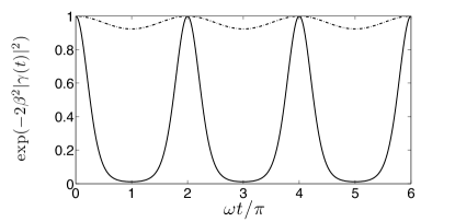
Figure 2: The time evolution of exp$(-2\beta^{2}|\gamma(t)|^{2})$ for (solid line) $\beta=0.75$ and (dotted-dashed line) $\beta=0.1$.

The integral in Eq.(11) is a two dimensional Fourier transform of $P$. So for each initial field, one needs to use its corresponding $P$ representation and calculate its two dimensional Fourier transform and hence $Q(t)$. In Eq.(11) all time dependences are captured in terms of $\gamma(t)$ and $\gamma^{*}(t)$. This guarantees that irrespective of the initial state the value of Eq.(11) is a periodic function with the period $T=2\pi/\omega$. The periodic dynamics is a manifestation of the fact that, in the degenerate regime, the JC Hamiltonian becomes a doubly degenerate harmonic oscillator. Furthermore, the periodic modulating factor, $\text{exp}({-2\beta^{2}|\gamma(t)|^{2}})$, is present irrespective of the initial field state. In Fig. 2 we have plotted the evolution of this factor for different values of $\beta$. This factor comes from the inner product between two coherent states in Eq.(10). These two coherent states came from the evolution of $|\uparrow,\alpha\rangle$ and $|\downarrow,\alpha\rangle$. The average complex excitation amplitudes of these two coherent states are $\alpha$ initially. As time increases these average excitation amplitudes follow two different circles in the complex plane and if $\beta\gtrsim 0.75$ these coherent states become effectively orthogonal to each other and their inner product becomes much smaller than 1. At $t=2\pi/\omega$ the average excitation amplitudes become $\alpha$ again and that is when the modulating factor becomes 1. The periodic damping in the modulating envelope (Fig.2) is a manifestation of this effective orthogonality.

IV Entanglement Dynamics

The system we choose to study consists of two non-communicating subsystems, labeled as $Aa$ and $Bb$. Each subsystem itself consists of a qubit, labeled as $A$ and $B$, each interacts with a partner field, labeled as $a$ and $b$. In figure Fig. 3 we show a schematic representation of the setup whose entanglement dynamics we seek to analyze. A particular point for attention is whether the initial entanglement shared between two remote systems dies out in a finite period of time, a phenomenon called early stage disentanglement or entanglement sudden death (ESD) Yu and Eberly (2009).

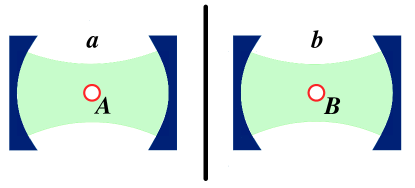
Figure 3: A schematic representation of the setup where two remote qubits are interacting with their own environments. There is no interaction between remote parties. Two qubits are assumed to be initially maximally entangled and the fields are in individual separable states.

The Hamiltonian of the system can be written as the sum of the Hamiltonians of each subsystem. The Hamiltonian of each subsystem is a JC Hamiltonian in the degenerate regime:

$$H=2\hbar\frac{\lambda}{\omega^{2}}+\sum_{i=1,2}\Bigg{(}\hbar\omega a^{\dagger}_{i}a_{i}+\hbar g(a_{i}^{\dagger}+a_{i})\sigma_{x}^{(i)}\Bigg{)}.$$ (12)

Two qubits, $A$ and $B$, are assumed to be initially maximally entangled and separable from the fields. After $t=0$ each qubit interacts with its partner field.

The initial qubit states under consideration are

$$|\Phi_{\pm}\rangle=\frac{|e,e\rangle\pm|g,g\rangle}{\sqrt{2}}.$$ (13)

These are the maximally entangled Bell states that were invoked in previous investigations Yönaç et al. (2006, 2007) for a similar scenario in the RWA regime Yönaç et al. (2006). Two other Bell states

$$|\Psi_{\pm}\rangle=\frac{|e,g\rangle\pm|g,e\rangle}{\sqrt{2}}$$ (14)

are not considered separately since in the degenerate regime there is no difference between the entanglement dynamics of $|\Phi_{\pm}\rangle$ and $|\Psi_{\pm}\rangle$. To see the reason for this note that

$$\sigma_{x}^{(1)}U|\Phi_{\pm}\rangle\otimes|\Lambda_{a},\Lambda_{b}\rangle=U|\Psi_{\pm}\rangle\otimes|\Lambda_{a},\Lambda_{b}\rangle,$$ (15)

where we used the fact that $[\sigma^{(1)},H]=0$ and $|\Lambda_{a},\Lambda_{b}\rangle$ can be any combination of initial pure field states. Thus, there is a local unitary transformation that brings the state that is produced by the initial state $|\Phi_{\pm}\rangle$ to the state that is the result of the propagation of $|\Psi_{\pm}\rangle$. This means that these two states have the same entanglement Horodecki et al. (2009). This result can be readily generalized for all initial states. Throughout this section, where it is needed to quantify entanglement, we take advantage of Wootters concurrence Wootters (1998) as is already used in the RWA regime Yönaç et al. (2006).

To find the reduced density matrix of two qubits, $Q^{\pm}(t)$, one can generalize the technique we employed in the previous section. We assume that at $t=0$ the qubits are entangled with each other but are separable from the fields and furthermore, two fields are initially separable too. Thus, the density matrix of the system can be written as

$$\rho_{ABab}^{\pm}(0)=|\Phi_{\pm}\rangle\langle\Phi_{\pm}|\otimes F_{a}\otimes F_{b}.$$ (16)

If we use the $|\uparrow\uparrow\rangle$,$|\uparrow\downarrow\rangle$, $|\downarrow\uparrow\rangle$ and $|\downarrow\downarrow\rangle$ basis, the diagonal terms of $Q^{\pm}(t)$ remain constant. In $Q^{+}(t)$ the only non-vanishing off-diagonal elements are $Q_{\uparrow\uparrow,\downarrow\downarrow}^{+}(t)$ and its conjugate. In $Q^{-}(t)$, however, the only non-vanishing off-diagonal elements are $Q_{\uparrow\downarrow,\downarrow,\uparrow}^{-}(t)$ and its conjugate. Here, for simplicity, we assume the initial fields are identical. If the $P$ representation of the initial fields is $P(\alpha)$, then it can be shown that

$$Q_{\uparrow\uparrow,\downarrow\downarrow}^{+}(t) =\frac{e^{-4\beta^{2}|\gamma(t)|^{2}}}{2}\left(\int\text{d}^{2}\alpha P(\alpha)e^{4i\beta Im[\alpha\gamma^{*}(t)]}\right)^{2},$$

$$Q_{\uparrow\downarrow,\downarrow\uparrow}^{-}(t) =\frac{e^{-4\beta^{2}|\gamma(t)|^{2}}}{2}~{}\left|\int\text{d}^{2}\alpha P(\alpha)e^{4i\beta Im[\alpha\gamma^{*}(t)]}\right|^{2}.$$ (17)

Now for each choice of initial field one can evaluate the integral and through it find $Q(t)$. For the above initial conditions, the concurrence also takes a very simple form:

$$C_{AB}^{+}(t)=C_{AB}^{-}(t)=2|Q_{\uparrow\uparrow,\downarrow\downarrow}^{+}(t)|=2|Q_{\uparrow\downarrow,\downarrow\uparrow}^{-}(t)|.$$ (18)

The fact that concurrence depends only on the absolute value of $Q_{\uparrow\uparrow,\downarrow\downarrow}^{+}(t)$ guarantees that the evolution of concurrence is the same for $|\Phi_{\pm}\rangle$ states. For simplicity from now on we drop the subscript $AB$ and superscripts $\pm$ and focus only on the state $|\Phi_{+}\rangle$.

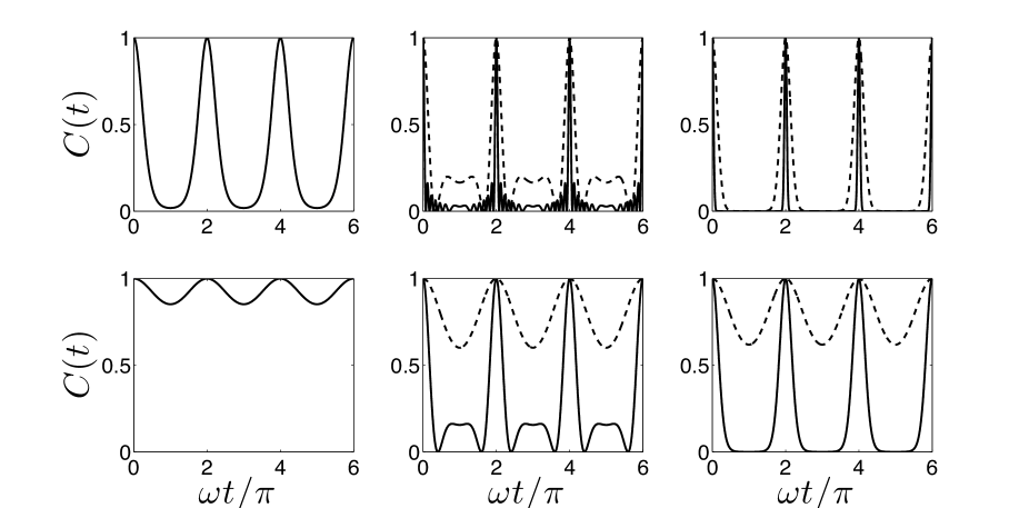
Figure 4: The evolution of concurrence between two qubits in the degenerate regime for different initial fields and different coupling strength. In the top row we used $\beta=0.5$ and for the bottom row $\beta=0.1$. In the left column the two initial fields are assumed to be in coherent states. In the middle column two initial fields are initially in number states (solid) N=25 and (dashed) N=1. In the right column the initial fields are initially in thermal fields with (solid) $\bar{n}=25$ and (dashed) $\bar{n}=1$

Coherent states: We assume two fields are initially in identical coherent states $|\alpha_{0}\rangle$. The initial state of the whole system then reads

$$|\Phi_{+}\rangle\otimes|\alpha_{0}\rangle\otimes|\alpha_{0}\rangle.$$

In the degenerate regime the off-diagonal term, $Q_{\uparrow\uparrow,\downarrow\downarrow}(t)$, reads

$$Q_{\uparrow\uparrow,\downarrow\downarrow}(t)=\frac{1}{2}e^{8i\beta Im{[\alpha_{0}\gamma^{*}(t)]}}e^{-4\beta^{2}|\gamma(t)|^{2}}.$$ (19)

Thus, $\alpha_{0}$ only appears in a phase and this means the average excitation number of a coherent state does not have any effect on the concurrence. Thus, in the degenerate regime, the concurrence between two qubits that are coming in contact with two coherent fields, $C_{coh}(t)$, is the same as two qubits interacting with two initial vacuum fields. In Fig. 4 (left panel), we present the evolution of concurrence between qubits for a coherent state. As $\beta$ increases, the minimum of the concurrence decreases, but the change of $\alpha_{0}$ does not have any effect on the concurrence. At $\omega t=2k\pi$, where $k$ is a natural number, $\gamma(t)=0$ and the initial entanglement revives completely. This is a result of harmonic oscillation in the dynamics and independent of the initial state.

Number states: Next we focus on the initial fields being number states. Here also for simplicity we assume both initial fields are identical and the initial state is

$$|\Phi_{+}\rangle\otimes|N\rangle\otimes|N\rangle.$$

To derive the entanglement dynamics in the degenerate regime one can use the $P$ representation of a number state Scully and Zubairy (1997):

$$P_{N}(\alpha)=\frac{e^{\alpha\alpha^{*}}}{N!}\frac{\partial^{2N}}{\partial\alpha^{N}\partial\alpha^{*N}}\delta^{(2)}(\alpha)$$

and evaluate the integral in Eq.(17). It can be shown that

$$C_{N}(t)=e^{-4\beta^{2}|\gamma(t)|^{2}}[L_{N}(4\beta^{2}|\gamma(t)|^{2})]^{2},$$ (20)

where $L_{N}$ is a Laguerre polynomial. In Fig. 4 (middle column) we plotted $C_{N}(t)$ for different values of $N$. The complete restoration of the entanglement is again a signature of the harmonic oscillatior dynamics. As $\beta$ increases, $4\beta^{2}|\gamma(t)|^{2}$ reaches more zeros of $L_{N}$ in a period of oscillation and thus concurrence vanishes momentarily at more points of time. $L_{N}$ has only $N$ roots and thus the number of moments at which concurrence vanishes is at most $2N$. As $N$ increases, the two qubits spend less time remaining maximally entangled. Thus, for a thermal field which is a mixture of Fock states one would also expect the temporal width of the restoration to decrease as the average excitation number of the two fields increases.

Thermal states: In this section we assume that two fields are initially in identical thermal states. Thermal environments are typically associated with the loss of coherence in the system when it comes in contact with the environment. However, due to the harmonic nature of the degenerate regime we do expect a complete restoration of the concurrence when $\gamma(t)=0$. To study the entanglement dynamics in the degenerate regime we can invoke the $P$ representation of a thermal field Scully and Zubairy (1997):

$$P_{th}(\alpha)=\frac{1}{\pi\bar{n}}\text{exp}(-|\alpha|^{2}/\bar{n}).$$

The integral in Eq.(17) becomes a Gaussian integral. For two initially identical fields with average excitation $\bar{n}$, the concurrence between two qubits in the degenerate regime is given by

$$C_{th}(t)=\text{exp}(-4(1+2\bar{n})\beta^{2}|\gamma(t)|^{2}).$$ (21)

As argued before, by increasing the average excitation number of thermal fields the temporal width of the restoration period decreases. This can also be understood in terms of coherent states. To the off-diagonal elements of the density matrix of two qubits, each coherent state contributes a specific phase $\text{exp}(8i\beta Im{[\alpha\gamma^{*}(t)]})$. As $\bar{n}$ increases the width of the Gaussian in the complex plane increases and more $\alpha$’s contribute significantly to the integral in Eq.(17). This leads to a faster collapse of $C_{th}(t)$ as $\gamma(t)$ becomes non-zero. In other words as a Gaussian broadens in the $\alpha$ domain, its Fourier transform becomes narrower. From Eq.(17) one can conclude that the effect of the average excitation number in the thermal field is the same as to enhance the coupling $\beta$. In Fig. 4 (right column) $C_{th}(t)$ is presented for different values of $\bar{n}$. It is interesting that for a weak coupling and far from the resonance if the fields are thermally excited enough, i.e. $8\bar{n}\beta^{2}\gtrsim 1$, then the fields effect both the local-coherences and entanglement between two qubits considerably in a short time.

For all the initial states we studied so far, the concurrence is an explicit function of $4\beta^{2}|\gamma(t)|^{2}$. This control quantity is a periodic function in time and it also depends explicitly on $\beta$. Our treatment of the degenerate regime does not impose any constraint on the value of $\beta$. Here we fix a time and study the effect of the coupling strength on the concurrence. We study the effect of $\beta$ at time $t=\frac{\pi}{\omega}$, when the control quantity, $4\beta^{2}|\gamma(t)|^{2}$, takes its maximum value $16\beta^{2}$. One can show that at $t=\frac{\pi}{\omega}$

$$C_{coh}(\pi/\omega) =e^{-16\beta^{2}},$$

$$C_{N}(\pi/\omega) =e^{-16\beta^{2}}[L_{N}(16\beta^{2})]^{2},$$

$$C_{th}(\pi/\omega) =e^{-16\beta^{2}(1+2\bar{n})}.$$ (22)

In Fig. 5 we plot the concurrence at $t=\frac{\pi}{\omega}$ versus $\beta$. As $\beta$ increases the concurrence decreases exponentially. The initial excitation in coherent states, (top panel), does not effect the concurrence. In the middle panel we plot the concurrence for the number state fields. The effect of the number state excitation is captured in the Laguerre polynomial modulation of the exponential decay. As we see in the bottom panel, increasing the average excitation number in thermal fields enhances the exponential decrease of the concurrence.

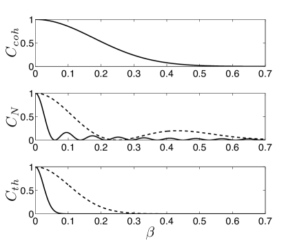
Figure 5: Concurrence between two qubits, evaluated at $t=\pi/\omega$, as a function of $\beta$. Top, we presented the concurrence when the initial fields are identical coherent states. Middle row, presented is the concurrence when the initial fields are number states (solid) N=25 and (dashed) N=1. Bottom, we presented the concurrence when the initial fields are identical thermal fields (solid) $\bar{n}=25$ and (dashed) $\bar{n}=1$.

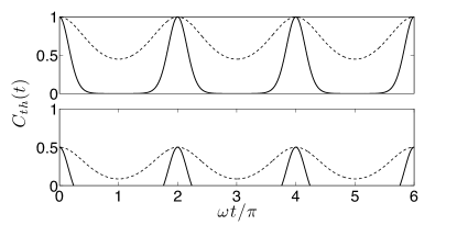
Figure 6: The evolution of concurrence between two qubits in the degenerate regime for $\beta=0.1$. In the top the initial fields are identical thermal fields with (solid) $\bar{n}=25$ and (dashed) $\bar{n}=2$. In the bottom we presented $C_{th}(t)$ for the initial thermal fields and qubits are initially in the state described in Eq.(23) in degenerate regime. (solid) $\bar{n}=25$ and (dashed) $\bar{n}=2$.

Next we focus on the phenomenon of ESD Yu and Eberly (2009). From Eq.(21) one sees that $C_{th}(t)>0$, so irrespective of how strong the coupling is, ESD does not happen in the degenerate regime. Increasing the coupling strength only decreases the minimum of the entanglement. It shall be pointed out that this is an artifact of the initial qubit state that was chosen and is not a generic property of the degenerate regime. The reason that this initial state does not show ESD is that in the basis $|\uparrow\uparrow\rangle$,$|\uparrow\downarrow\rangle$, $|\downarrow\uparrow\rangle$ and $|\downarrow\downarrow\rangle$, two of the diagonal terms of the density matrix $Q(t)$ are zero. Thus to have ESD the off-diagonal element, $Q_{\uparrow\uparrow,\downarrow\downarrow}(t)$, should vanish for a finite time interval, but this element does not vanish.

In Fig. 6, along with $C_{th}(t)$ for $|\Phi_{+}\rangle$, we also plot $C_{th}(t)$ when the qubits share the initial state

$$Q(0)=\frac{3}{4}|\Phi_{+}\rangle\langle\Phi_{+}|+\frac{1}{8}|\uparrow\downarrow\rangle\langle\uparrow\downarrow|+\frac{1}{8}|\downarrow\uparrow\rangle\langle\downarrow\uparrow|.$$ (23)

For this initial state, if $\beta$ is big enough, two qubits become disentangled for a finite period of time and thus ESD happens.

So far we studied the evolution of the bipartite entanglement between two qubits and focused on the effect of the local environments on $C(t)$. The question that arises is how does the this entanglement get transferred between the different parties involved? In the RWA regime, the question is answered for the case when the initial fields are in the vacuum Yönaç et al. (2007). They showed that after $t=0$ the interaction between each qubit and the corresponding field leads to the development of non-local bipartite entanglement between two non-local fields. In what follows we show that in the degenerate regime, irrespective to how strong the coupling is, and what the initial fields are, the two initially separable non-local fields do not develop bipartite entanglement.

To this end, assume the initial fields to be two vacuum fields so that the initial state of the system reads

$$|\Phi_{+}\rangle\otimes|0,0\rangle=\frac{1}{\sqrt{2}}\Big{(}|\uparrow\uparrow\rangle+|\downarrow\downarrow\rangle\Big{)}\otimes|0,0\rangle.$$ (24)

After $t=0$, each qubit interacts with the corresponding field. Therefore at $t>0$ the state of the system is given by

$$U|\Phi_{+}\rangle\otimes|0,0\rangle=\frac{|\uparrow\uparrow,\beta(t),\beta(t)\rangle+|\downarrow\downarrow,-\beta(t),-\beta(t)\rangle}{\sqrt{2}},$$ (25)

where $|\pm\beta(t)\rangle$ are coherent states and $\beta(t)=\beta(e^{-i\omega t}-1)=\beta\gamma^{*}(t)$. For the above state if two qubits are traced out, the reduced density matrix of the two fields is separable. In other words at any moment an observer can measure the state of the qubits in the basis $|\uparrow\uparrow\rangle$, $|\uparrow\downarrow\rangle$, $|\downarrow\uparrow\rangle$ and $|\downarrow\downarrow\rangle$ and by knowing the result one can also tell the state of each field. One can readily generalize the above result to any initial state for which the fields are separable from each other and from the qubits.

The question that remains is the destination of initial entanglement. To where is it transferred? For the initial condition we studied above, if the coupling is strong enough such that $\left\langle\beta(t)|-\beta(t)\right\rangle\approx 0$, then the initial bipartite entanglement between two qubits becomes a pure 4-partite entanglement between all the parties involved and there remains no bipartite entanglement in the system.

V conclusion

In this report we studied the excitation exchange and entanglement dynamics in the Jaynes-Cummings model far from the RWA regime. In the degenerate regime, the dynamics can be understood as displaced harmonic oscillations of the field around a center that depends on the qubit state. This leads to complete restoration of coherences irrespective of the initial state.

We also invoked a previously studied model Yönaç et al. (2007) and studied the entanglement dynamics for two remote qubits that are interacting with two local environments in the degenerate regime. We assumed that initially the qubits are separable from the environments and of all initial qubit states we chose to focus on the Bell states. It was shown that $|\Psi_{\pm}\rangle$ has the same entanglement dynamics as $|\Phi_{\pm}\rangle$. Different choices of single mode environments were examined. We showed that the effect of all coherent states on the concurrence is the same as the effect of the vacuum state and initial excitation in a coherent state does not have any effect on the bipartite entanglement between two qubits. In cases of number state and thermal fields the initial excitation of the fields does effect the evolution of concurrence between two qubits. In the case of thermal fields, the effect can be captured as an enhancement of the coupling between each qubit and the corresponding field. The fact that a highly excited thermal field can, in a short time, affect the local and non-local coherences of a degenerate off-resonance qubit that is weakly coupled to it and a highly excited coherent state can not, is of importance.

In another sharp contrast to the previously studied scenario Yönaç et al. (2007), it was shown that no bipartite entanglement can be induced between two remote fields using the initial entanglement between two qubits in degenerate regime. This raises a question about the quasi-degenerate regime that remains to be considered for future investigation. The question is, for the regime where the degeneracy of the qubits is broken with a small splitting $\omega_{o}\ll\omega,\lambda$, can the initial entanglement between two qubits induce a non-zero bipartite entanglement between two fields. If yes, then is there a limit on the amount of this induced entanglement or not, and in what time scale does the entanglement get transferred? Finally, for the initial state that we examined, all the initial entanglement transformed to a 4-partite entanglement between all parties involved. The presented scenario can also be thought of as a scenario to produce pure 4-partite entanglement which is potentially useful in the studies of multi-partite entanglement.

VI acknowledgement

We acknowledge partial financial support from ARO W911NF-09-1-0385 and NSF PHY-0601804.

VII Appendix A

In this section we prove the equation 8. We are interested in finding the evolution of $|\uparrow,\alpha\rangle$. Note that

$$U|\uparrow,\alpha\rangle=|\uparrow\rangle\otimes D(\beta)^{\dagger}e^{-i\omega ta^{\dagger}a}D(\beta)|\alpha\rangle$$

$$=|\uparrow\rangle\otimes D(\beta)^{\dagger}e^{-i\omega ta^{\dagger}a}|(\alpha+\beta)\rangle e^{iIm{(\beta\alpha^{*})}}$$

$$=|\uparrow\rangle\otimes D(\beta)^{\dagger}|(\alpha+\beta)e^{-i\omega t}\rangle e^{iIm{(\beta\alpha^{*})}}$$

$$=|\uparrow\rangle\otimes|(\alpha+\beta)e^{-i\omega t}-\beta\rangle e^{-i\beta^{2}\sin\omega t}e^{-i\beta Im(\alpha^{*}(e^{i\omega t}-1))}$$

$$=|\uparrow,(\alpha+\beta)e^{-i\omega t}-\beta\rangle e^{-i\beta^{2}\sin\omega t}e^{\frac{1}{2}\beta\alpha\gamma^{*}(t)}e^{-\frac{1}{2}\beta\alpha^{*}\gamma(t)}$$

$$=|\uparrow,(\alpha+\beta)e^{-i\omega t}-\beta\rangle e^{-i\beta^{2}\sin\omega t}e^{i\beta Im[\alpha\gamma^{*}(t)]}.$$

In deriving the above result it is assumed that $\beta$ is a real number. The evolution of the state $|\downarrow,\alpha\rangle$ can be worked out in a similar way.

References

- Nielsen and Chuang (2000) M. A. Nielsen and I. L. Chuang, Quantum Computation and Quanum Information (Cambridge U.P., 2000).
- Horodecki et al. (2009) R. Horodecki, P. Horodecki, M. Horodecki, and K. Horodecki, Rev. Mod. Phys. 81, 865 (2009).
- Raimond et al. (2001) J. M. Raimond, M. Brune, and S. Haroche, Rev. Mod. Phys. 73, 565 (2001).
- Benatti et al. (2003) F. Benatti, R. Floreanini, and M. Piani, Phys. Rev. Lett. 91, 070402 (2003).
- Braun (2002) D. Braun, Phys. Rev. Lett. 89, 277901 (2002).
- Kim et al. (2002) M. S. Kim, J. Lee, D. Ahn, and P. L. Knight, Phys. Rev. A 65, 040101 (2002).
- Tessier et al. (2003) T. E. Tessier, I. H. Deutsch, A. Delgado, and I. Fuentes-Guridi, Phys. Rev. A 68, 062316 (2003).
- Anastopoulos et al. (2009) C. Anastopoulos, S. Shresta, and B. Hu, Quant. Inf. Process. 8, 549 (2009).
- Ficek (2010) Z. Ficek, Opt. Spect. 108, 347 (2010).
- Yu and Eberly (2004) T. Yu and J. H. Eberly, Phys. Rev. Lett. 93, 140404 (2004).
- Yönaç et al. (2006) M. Yönaç, T. Yu, and J. H. Eberly, J. Phys. B 39, S621 (2006).
- Bellomo et al. (2007) B. Bellomo, R. Lo Franco, and G. Compagno, Phys. Rev. Lett. 99, 160502 (2007).
- Al-Qasimi and James (2008) A. Al-Qasimi and D. F. V. James, Phys. Rev. A 77, 012117 (2008).
- Chruściński and Kossakowski (2010) D. Chruściński and A. Kossakowski, Phys. Rev. Lett. 104, 070406 (2010).
- Liu and Goan (2007) K.-L. Liu and H.-S. Goan, Phys. Rev. A 76, 022312 (2007).
- López et al. (2008) C. E. López, G. Romero, F. Lastra, E. Solano, and J. C. Retamal, Phys. Rev. Lett. 101, 080503 (2008).
- Yönaç and Eberly (2010) M. Yönaç and J. H. Eberly, Phys. Rev. A 82, 022321 (2010).
- Jaynes and Cummings (1963) E. Jaynes and F. Cummings, Proc. IEEE 51, 89 (1963).
- Allen and Eberly (1987) L. Allen and J. H. Eberly, Optical Resonance and Two-Level Atoms (Dover Publications, 1987).
- Irish and Schwab (2003) E. K. Irish and K. Schwab, Phys. Rev. B 68, 155311 (2003).
- Blais et al. (2004) A. Blais, R.-S. Huang, A. Wallraff, S. M. Girvin, and R. J. Schoelkopf, Phys. Rev. A 69, 062320 (2004).
- Wallraff et al. (2004) A. Wallraff, D. I. Schuster, A. Blais, L. Frunzio, R.-S. Huang, J. Majer, S. Kumar, S. M. Girvin, and R. J. Schoelkopf, Nature 431, 162 (2004).
- Niemczyk et al. (2010) T. Niemczyk, F. Deppe, H. Huebl, E. P. Menzel, F. Hocke, M. J. Schwarz, J. J. García-Ripoll, D. Zueco, T. Hummer, E. Solano, A. Marx, and R. Gross, Nat. Phys. 6, 772 (2010).
- Fedorov et al. (2010) A. Fedorov, A. K. Feofanov, P. Macha, P. Forn-Díaz, C. J. P. M. Harmans, and J. E. Mooij, Phys. Rev. Lett. 105, 060503 (2010).
- Forn-Díaz et al. (2010) P. Forn-Díaz, J. Lisenfeld, D. Marcos, J. J. García-Ripoll, E. Solano, C. J. P. M. Harmans, and J. E. Mooij, Phys. Rev. Lett. 105, 237001 (2010).
- Shore (1990) B. W. Shore, The Theory of Coherent Atomic Excitation: Vol. 1, Simple Atoms and Fields (Wiley-Intersceience Publication, 1990) Chap. 4.
- Swain (1973) S. Swain, J. Phys. A: Math. Nucl. Gen. 6, 192 (1973).
- Crisp (1992) M. D. Crisp, Phys. Rev. A 46, 4138 (1992).
- Klimov et al. (2003) A. B. Klimov, I. Sainz, and S. M. Chumakov, Phys. Rev. A 68, 063811 (2003).
- Larson (2007) J. Larson, Phys. Scr. 76, 146 (2007).
- Zaheer and Zubairy (1988) K. Zaheer and M. S. Zubairy, Phys. Rev. A 37, 1628 (1988).
- Finney and Gea-Banacloche (1994) G. A. Finney and J. Gea-Banacloche, Phys. Rev. A 50, 2040 (1994).
- Irish (2007) E. K. Irish, Phys. Rev. Lett. 99, 173601 (2007).
- Irish et al. (2005) E. K. Irish, J. Gea-Banacloche, I. Martin, and K. C. Schwab, Phys. Rev. B 72, 195410 (2005).
- Casanova et al. (2010) J. Casanova, G. Romero, I. Lizuain, J. J. García-Ripoll, and E. Solano, Phys. Rev. Lett. 105, 263603 (2010).
- Hausinger and Grifoni (2010) J. Hausinger and M. Grifoni, Phys. Rev. A 82, 062320 (2010).
- Chen et al. (2010) Q.-H. Chen, Y. Yang, T. Liu, and K.-L. Wang, Phys. Rev. A 82, 052306 (2010).
- Shakov and McGuire (2003) K. K. Shakov and J. H. McGuire, Phys. Rev. A 67, 033405 (2003).
- Yönaç et al. (2007) M. Yönaç, T. Yu, and J. H. Eberly, J. Phys. B 40, S45 (2007).
- Glauber (1963) R. J. Glauber, Phys. Rev. 131, 2766 (1963).
- Sudarshan (1963) E. C. G. Sudarshan, Phys. Rev. Lett. 10, 277 (1963).
- Yu and Eberly (2009) T. Yu and J. H. Eberly, Science 323, 598 (2009).
- Wootters (1998) W. K. Wootters, Phys. Rev. Lett. 80, 2245 (1998).
- Scully and Zubairy (1997) M. O. Scully and M. S. Zubairy, Quantum Optics (Cambridge University Press, 1997).