RU-NHETC-2011-9

Critical values of the Yang-Yang functional in the quantum sine-Gordon model

Sergei L. Lukyanov

NHETC, Department of Physics and Astronomy

Rutgers University

Piscataway, NJ 08855-0849, USA

and

L.D. Landau Institute for Theoretical Physics

Chernogolovka, 142432, Russia

Abstract

The critical values of the Yang-Yang functional corresponding to the vacuum states of the sine-Gordon QFT in the finite-volume are studied. Two major applications are discussed: (i) generalization of Fendley-Saleur-Zamolodchikov relations to arbitrary values of the sine-Gordon coupling constant, and (ii) connection problem for a certain two-parameter family of solutions of the Painlev${\acute{\rm e}}$ III equation.

1 Introduction

Throughout the past, a number of important facts about the quantum sine-Gordon model were discovered. Among them are elegant relations between the zero-point energy and the Painlev${\acute{\rm e}}$ III transcendent. To describe them explicitly let us recall some elementary facts about a structure of the Hilbert space of the model,

$$\mathcal{L}={\frac{1}{\beta^{2}_{\rm sg}}}\ \Big{(}\,\ {\frac{1}{2}}\ (\partial_{\mu}\phi)^{2}+\Lambda\ \cos(\phi)\,\Big{)}\ ,$$ (1.1)

in finite-size geometry with the spatial coordinate $x$ compactified on a circle of a circumference $R$, with the periodic boundary conditions

$$\phi(x+R,t)=\phi(x,t)\ .$$ (1.2)

Due to the periodicity of the potential term $\Lambda\,\cos(\phi)$ in (1.1) in $\phi$, the space of states $\mathcal{H}$ splits into orthogonal subspaces $\mathcal{H}_{k}$, characterized by the “quasi-momentum” $k$,

$$\phi\to\phi+2\pi\,:\qquad\mid\Psi_{k}\,\rangle\ \to\ \mbox{e}^{2\pi{\rm i}\,k}\,\mid\Psi_{k}\,\rangle$$ (1.3)

for $\mid\Psi_{k}\,\rangle\in\mathcal{H}_{k}$. We call $k$-vacuum the ground state of the finite-size system (1.1) in the sector $\mathcal{H}_{k}$ and denote it by $|\,\Psi^{{\rm(vac)}}_{k}\,\rangle$. The corresponding energy will be denoted by $E_{k}$.

In general, the coupling constant in (1.1) should be restricted by the condition $\beta^{2}_{\rm sg}<8\pi$ [1] and it is convenient to substitute $\beta^{2}_{\rm sg}$ for the “renormalized coupling”:

$$\xi=\frac{\beta^{2}_{\rm sg}}{8\pi-\beta^{2}_{\rm sg}}\ .$$ (1.4)

The value $\xi=2$ is special. For this coupling, the theory possesses ${\cal N}=2$ supersymmetry which is spontaneously broken, except the subspaces $\mathcal{H}_{k}$ corresponding to $k=\pm\frac{1}{4}$ [2]. In the sectors with unbroken supersymmetry the ground state energy is of course identically zero. In Ref.[3] Fendley and Saleur (see also related Ref.[4]) applied the general construction [5] to derive the remarkable relation

$$\frac{R}{\pi}\ \Big{(}\frac{\partial E_{k}}{\partial k}\Big{)}_{\xi=2\atop k=\pm 1/4}=\mp 4r\,\frac{\mbox{d}U(r)}{\mbox{d}r}\ .$$ (1.5)

Here the variable $r$ stands for the size of the system measured in the units of the correlation length (inverse soliton mass $M$),

$$r=MR\ ,$$ (1.6)

and $U=U(t)$ is a particular solution to the Painlev${\acute{\rm e}}$ III equation

$$\frac{1}{t}\ \frac{\mbox{d}}{\mbox{d}t}\Big{(}t\,\frac{\mbox{d}U}{\mbox{d}t}\Big{)}=\frac{1}{2}\ \sinh(2U)\ .$$ (1.7)

This equation admits a one-parameter family of solutions regular at $t>0$ (see e.g.[6]) called the Painlev${\acute{\rm e}}$ III transcendents. The special solution in (1.5) is fixed by the following boundary conditions

$$U(t)=\begin{cases}-\frac{1}{3}\ \log(t)+O(1)\ \ \ \ \ {\rm as}\ \ \ \ t\to 0\\ \ o(1)\ \ \ \ \ \ \ \ \ \ \ \ \ \ \ \ \ \ \ \ \ \ {\rm as}\ \ \ \ t\to\infty\end{cases}\ .$$ (1.8)

In the consequent work [7] Alyosha Zamolodchikov derived one more mysterious relation

$$\frac{R}{\pi}\ \Big{(}\frac{\partial E_{k}}{\partial\xi}\Big{)}_{\xi=2\atop k=\pm 1/4}=-\frac{r^{2}}{8}+\frac{1}{2}\ \int_{r}^{\infty}\mbox{d}t\ t\ \sinh^{2}U(t)\ .$$ (1.9)

Below, we will refer to Eqs. (1.5), (1.9) as the FSZ relations.

Relations similar to (1.5) and (1.9) were also discovered in other models [4], [8], [9]. However all the generalizations had limitations in the choice of coupling constants and sectors of the theories. The long-time consensus was the FSZ relations are due to the accidental symmetry and do not possess any interesting generalizations for general values of $\xi$ and $k$. The first serious sign that this may not be true came from the study of $D=4$ supersymmetric gauge theories [11, 12, 13, 14, 15]. In these works a link was observed between certain Thermodynamic Bethe Ansatz (TBA) type integral equations and partial differential equations integrated by the inverse scattering methods. Some of the integral equations were in fact identical to the sine-Gordon TBA systems corresponding to $\xi\not=2$ and $k\not=\pm\frac{1}{4}$. Inspired by this remarkable development, A. Zamolodchikov and the author found a classical integrable equation associated with the quantum sine-Gordon model for generic $\xi$ and $k$ [10]. It turned out to be the classical Modified Sinh-Gordon equation (MShG)

$$\partial_{z}\partial_{\bar{z}}\eta-\mbox{e}^{2\eta}+p(z)\,{p}({\bar{z}})\ \mbox{e}^{-2\eta}=0$$ (1.10)

with $p(z)$ of the form

$$p(z)=z^{2\alpha}-s^{2\alpha}\,.$$

Parameters $\alpha$ and $s$ are real and positive, related to the sine-Gordon parameters $\xi$ (1.4) and $r=MR$ (1.6) as follows

$$\alpha={\xi}^{-1}\ ,\ \ \ \ \ \ \qquad\qquad s=\Big{(}\frac{2\,r}{\xi\,r_{\xi}}\Big{)}^{\frac{\xi}{1+\xi}}\ ,$$ (1.11)

where, for future references, we use the notation

$$r_{\xi}=\frac{2\sqrt{\pi}\,\Gamma(\frac{\xi}{2})}{\Gamma(\frac{3}{2}+\frac{\xi}{2})}\ .$$ (1.12)

The MShG equation in general has no rotational symmetry. Instead, it has the discrete symmetry $z\to\text{e}^{\frac{{\rm i}\pi}{\alpha}}\,z\,,\ {\bar{z}}\to\text{e}^{-\frac{{\rm i}\pi}{\alpha}}\,{\bar{z}}$. Solutions of the MShG equation (1.10) relevant to the problem respect this symmetry, are continuous at all finite nonzero $z$, and grow slower then the exponential as $|z|\to\infty$. In other words, they are single-valued functions on a cone with the apex angle $\frac{\pi}{\alpha}$ including the zero of $p(z)$ (see Fig.1). There is a one-parameter family of such solutions, characterized by the behavior at the apex: $\eta\to 2l\,\log|z|+O(1)$ as $|z|\to 0$, with real $l\in(-\frac{1}{2},\,\frac{1}{2}\,)$ which turns out to be related to the quasi-momentum (1.3) by

$$l=2\,|k|-{\textstyle\frac{1}{2}}\ .$$ (1.13)

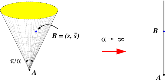
Figure 1: The world sheet for the MShG equation (1.10). The dots $A$ and $B$ indicate positions of the apex and zero of $p(z)$, respectively. At the minisuperspace limit ($\alpha\to\infty$, $r$ is kept fixed) the world sheet shrinks to a single ray.

The MShG equation can be represented as a flatness condition for certain $SL(2)$ connection. In Ref.[10] it was shown that the monodromy from the apex to infinity corresponding to the above described solution is essentially the sine-Gordon $Q$-function, whose asymptotic expansions generate the vacuum eigenvalues of integrals of motions of the quantum theory.

The original motivation for the present work was to incorporate the FSZ relations to the construction of Ref.[10]. This problem is solved in Section 2 of this work. It turned out that the main player in the derivation of the generalized FSZ relations is a properly defined “on-shell” action for the MShG equation. Remarkably it can also be interpreted as a critical value of the Yang-Yang (YY) functional in the quantum sine-Gordon model.

In the seminal work [16] the variational principle was applied to prove an existence of a solution to vacuum Bethe Ansatz (BA) equations for the XXZ spin chain. From that time the functional whose extremum condition reproduce BA equations bears the Yang-Yang name. The YY-functional proves to be useful for computing norms of the Bethe states (see e.g. [17] and references therein). Recently it attracts a great deal of attention in the context of the relation between supersymmetric gauge theories and quantum mechanical integrable systems [18, 19, 20]. However, the r${\hat{\rm o}}$le of the YY-functional in 2D QFT seems to be undervalued. To the best of my knowledge, it was never defined in intrinsic terms of integrable QFT. Nevertheless, there is a brute-force approach for the calculation of critical values of the YY-functional in the sine-Gordon QFT. It is based on the discretization of the theory, i.e., reducing it to the system with finite number of degrees of freedom, which then can be solved by standard methods of BA. Although this formal approach does not clarify the meaning of the YY-functional itself, it is sufficient for the calculation of the YY-functions, i.e., the critical values of YY-functional corresponding to the Bethe states. In this work we restrict our attention to the $k$-vacuum state $\mid\Psi^{{\rm(vac)}}_{k}\,\rangle\in\mathcal{H}_{k}$. In Section 3 it is shown that the corresponding YY-function can be identified with the on-shell action for the MShG equation. Another purpose of Section 3 is to discuss technical tools for the calculation of the YY-function. We review the well-known approach [21, 22] which allows one to express partial derivatives of the YY-function in terms of a solution to the non-linear integral equation from Ref.[22].

Section 4 is devoted to the so-called minisuperspace approximation (in the stringy terminology). The approximation implies the $\xi\to 0$ limit such that the soliton mass $M$ is kept fixed. In this case the sine-Gordon QFT reduces to the quantum mechanical problem of particle in the cosine potential. At the minisuperspace limit the world sheet of the MShG equation collapses into a single ray (see Fig. 1) and the solution $\eta$ at the segment $(A,\,B)$ is expressed in terms of a solution of the Painlev${\acute{\rm e}}$ III equation (1.7), subject of the boundary conditions

$$U(t)=\begin{cases}\ 2l\,\log(t)+O(1)\,\ \ \ \ \ \ \ \ {\rm as}\ \ \ \ t\to 0\\ -\log(r-t)+O(1)\ \ \ \ \ {\rm as}\ \ \ \ t\to r\end{cases}\ .$$ (1.14)

Real solutions of the Painlev${\acute{\rm e}}$ III equation which are regular at the open segment $t\in(0,r)$, and satisfy the boundary conditions (1.14), form a family which is parameterized by $r>0$ and $-\frac{1}{2}<l<\frac{1}{2}$. By taking the minisuperspace limit of the generalized FSZ relation, we solve the connection problem for the local expansions of the solution $U(t)$ (1.14) at $t=0$ and $t=r$. The results obtained in Section 4 provide an interesting link between the Painlev${\acute{\rm e}}$ III and Mathieu equations.

2 On-shell action for the ShG equation

2.1 From MShG to ShG

In practical calculations it is convenient to trade the world sheet variable $z$ in the MShG equation (1.10) to

$$w=\mbox{e}^{\frac{{\rm i}\pi(\alpha+1)}{2\alpha}}\ \int\mbox{d}z\ \sqrt{p(z)}\ ,$$ (2.1)

and similarly for ${\bar{w}}$. The branch of the multivalued function (2.1) can be chosen to provide the map of the cone with the cut along the ray $(AB)$ visualized in Fig.2a to the domain of the $w$-complex plane in Fig.2b (see Ref. [10] for details).

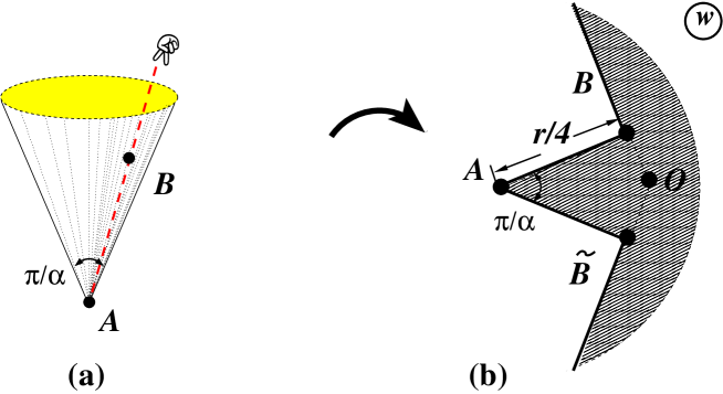
Figure 2: The $w$-image of the cutted cone under the map (2.1). The points on the cone and their images are denoted by the same symbols. The segment $A{\tilde{B}}$ is identified with $AB$, and the boundary line from ${\tilde{B}}$ to infinity is identified with the line from $B$ to infinity. The point $O$ is an origin of the $w$-plane.

This conformal map brings the MShG equation to the conventional Sinh-Gordon (ShG) form

$$\partial_{w}{\partial}_{\bar{w}}{\hat{\eta}}-\mbox{e}^{2{\hat{\eta}}}+\mbox{e}^{-2{\hat{\eta}}}=0$$ (2.2)

for ${\hat{\eta}}=\eta-{\textstyle\frac{1}{4}}\ \log\big{(}\,p(z)p({\bar{z}})\,\big{)}$, which vanishes at infinity

$$\lim_{|w|\to\infty}{\hat{\eta}}=0\ ,$$ (2.3)

becoming singular at the apex

$${\hat{\eta}}=2l\ \log|w-w_{A}|+O(1)\ \ \ \ \ {\rm as}\ \ \ \ \ |w-w_{A}|\to 0$$ (2.4)

and at the point $B\sim{\tilde{B}}$

$${\hat{\eta}}=-\frac{1}{3}\ \log|w-w_{B}|+O(1)\ \ \ \ \ {\rm as}\ \ \ \ \ |w-w_{B}|\to 0\ .$$ (2.5)

Unlike the apex singularity, the asymptotic (2.5) is an artifact of the coordinate transformation (2.1).

2.2 Action functional

To generalize relations (1.5), (1.9) we need an extra ingredient – the “on-shell” action for the ShG equation (2.2). It can be defined through the following limiting procedure. Start with the domain $D$ depicted in Fig.2b of the complex $w$-plane. Cut out the small sectors of radius $\epsilon$ around the point $A$, $B$ and ${\tilde{B}}$ to obtain the domain $D_{\epsilon}$ shown in Fig.3.

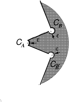
Figure 3: The integration domain $D_{\epsilon}$ for the regularized action (2.6).

Define the regularized action functional

$${\cal A}[\,{\hat{\eta}}\,] = \lim_{\epsilon\to 0}\,\bigg{[}\,\int_{D_{\epsilon}}\frac{\mbox{d}w\wedge\mbox{d}{\bar{w}}}{2\pi{\rm i}}\ \big{(}\,\partial_{w}{\hat{\eta}}\partial_{\bar{w}}{\hat{\eta}}+4\,\sinh^{2}({\hat{\eta}})\,\big{)}+\frac{l}{\pi\epsilon}\ \int_{C_{A}}\mbox{d}\ell\ {\hat{\eta}}-\frac{l^{2}}{\alpha}\ \log(\epsilon)$$ (2.6)

$$- \frac{1}{6\pi\epsilon}\ \int_{C_{B}}\mbox{d}\ell\ {\hat{\eta}}-\frac{1}{6\pi\epsilon}\ \int_{C_{{\tilde{B}}}}\mbox{d}\ell\ {\hat{\eta}}-\frac{1}{12}\ \log(\epsilon)\,\bigg{]}\ .$$

The first term is the “cutoff” version of the naive action for the ShG equation (2.2). The additional terms involves integrals over three arcs $C_{A}$, $C_{B}$ and $C_{{\tilde{B}}}$ and field-independent counterterms which provide an existence of the limit. Then the ShG equation supplemented by asymptotic behaviors near the singularities (2.4), (2.5) and at large $w$ (2.3) constitute a sufficient condition for an extremum of the functional (2.6):

$$\delta{\cal A}=0\ .$$ (2.7)

Finally we define the on-shell action ${\cal A}^{*}$ as the value of ${\cal A}[{\hat{\eta}}]$ calculated on the solution ${\hat{\eta}}$ (2.2)-(2.5).

For the variation (2.7) the world sheet geometry, as well as the parameter $l$ controlling the behavior of the solution at the apex, is assumed to be fixed. Varying the on-shell action with respect to the parameter $l$, it is observed that

$$\Big{(}\frac{\partial{\cal A}^{*}}{\partial l}\Big{)}_{r,\alpha}=\frac{1}{\alpha}\ {\hat{\eta}}_{A}\ ,$$ (2.8)

where the constant ${\hat{\eta}}_{A}$ can be thought of as a regularized value of the solution ${\hat{\eta}}$ at the apex

$${\hat{\eta}}_{A}=\lim_{|w-w_{A}|\to 0}\big{(}\,{\hat{\eta}}(w,{\bar{w}})-2l\,\log|w-w_{A}|\,\big{)}\ .$$ (2.9)

It should be stressed that unlike $l$, which is the “input” parameter applied with the problem, the value of the constant ${\hat{\eta}}_{A}$ is not prescribed in advance but determined through the solution, i.e. it is rather part of the “output”.

Let us consider now the infinitesimal variations of the world-sheet geometry. The corresponding $\delta{\cal A}$ do not vanish on-shell and can be expressed through the on-shell values of the stress-energy tensor. Under the infinitesimal dilation $\frac{\delta r}{r}=\frac{\delta\epsilon}{\epsilon}=\lambda\ll 1$,

$$\delta_{r}{\cal A}^{*}=\frac{\delta r}{r}\,\bigg{[}\,\lim_{\epsilon\to 0}\int_{D_{\epsilon}}\frac{\mbox{d}w\wedge\mbox{d}{\bar{w}}}{\pi{\rm i}}\ \Theta-\Big{(}\frac{l^{2}}{\alpha}+\frac{1}{12}\,\Big{)}\,\bigg{]}\ ,$$ (2.10)

where

$$\Theta=4\,\sinh^{2}({\hat{\eta}})$$ (2.11)

is a trace of the stress-energy tensor for the classical ShG equation. The other two non-vanishing components of $T_{\mu\nu}$ are given by

$$T=(\partial_{w}{\hat{\eta}})^{2}\,,\ \ \ \ \ \ \ {\bar{T}}=(\partial_{\bar{w}}{\hat{\eta}})^{2}\ .$$ (2.12)

By virtue of the ShG equation, they satisfy the continuity equations

$$\partial_{\bar{w}}T=\partial_{w}\Theta\ ,\ \ \ \ \ \partial_{w}{\bar{T}}=\partial_{\bar{w}}\Theta\ ,$$ (2.13)

and, hence, they can be expressed in terms of a single scalar potential

$$T=\partial^{2}_{w}\Phi\ ,\ \ \ \ \ {\bar{T}}={\bar{\partial}}^{2}_{w}\Phi\ ,\ \ \ \ \ \ \Theta=\partial_{w}\partial_{\bar{w}}\Phi\ .$$ (2.14)

Combining the last formula with (2.10), one has

$$r\,\Big{(}\frac{\partial{\cal A}^{*}}{\partial r}\Big{)}_{\alpha,l}=\lim_{\epsilon\to 0}\int_{D_{\epsilon}}\frac{\mbox{d}w\wedge\mbox{d}{\bar{w}}}{\pi{\rm i}}\ \partial_{w}\partial_{\bar{w}}\Phi-\Big{(}\frac{l^{2}}{\alpha}+\frac{1}{12}\,\Big{)}\ .$$ (2.15)

The 2-fold integral here can be reduced to the linear integral over the boundary of $D_{\epsilon}$. The linear integrals over the arcs $C_{A}$, $C_{B}$ and $C_{\tilde{B}}$ from Fig.3 cancel out the term in the brackets in (2.15). This follows from the asymptotic formulas

$${\Phi}(w,\,{\bar{w}})=-2l^{2}\ \log|w-w_{A}|+O(1)\ ,\ \ \ \ \ \ \ \ \ |w-w_{A}|\to 0$$ (2.16)

and

$${\Phi}(w,\,{\bar{w}})=-\frac{1}{18}\times\begin{cases}\log|w-w_{B}|+O(1)\ ,\ \ \ \ \ \ \ \ \ |w-w_{B}|\to 0\\ \log|w-w_{\tilde{B}}|+O(1)\ ,\ \ \ \ \ \ \ \ \ |w-w_{\tilde{B}}|\to 0\end{cases}\ ,$$ (2.17)

which are consequences of Eqs. (2.12), (2.14) and (2.4), (2.5). To proceed further, we need to use some properties of the potential $\Phi$ discussed in Appendix A. Namely, for $|w|>|w_{B}|$

$$\Phi\big{(}w\,\mbox{e}^{\frac{{\rm i}\pi(\alpha+1)}{\alpha}},\,{\bar{w}}\,\mbox{e}^{-\frac{{\rm i}\pi(\alpha+1)}{\alpha}}\,\big{)}=\Phi(w,\,{\bar{w}})$$ (2.18)

and

$$\lim_{|w|\to\infty}{\Phi}(w,\,{\bar{w}})=0\ .$$ (2.19)

Eq.(2.18) implies that the half-infinite boundary rays $(B,\,\infty)$ and $({\tilde{B}},\,\infty)$ from Fig.3 do not contribute into the integral (2.15). Now, taking into account Eq.(2.19), it is straightforward to show that

$$r\,\Big{(}\frac{\partial{\cal A}^{*}}{\partial r}\Big{)}_{\alpha,l}=-\frac{1}{2\pi}\ \sin\Big{(}{\frac{\pi}{2\alpha}}\Big{)}\ \big{(}\,{\mathfrak{J}}_{1}+{\bar{\mathfrak{J}}}_{1}\,\big{)}\ ,$$ (2.20)

where notations from Ref.[10] are adopted,

$$\sin\big{(}{\textstyle\frac{\pi}{2\alpha}}\big{)}\ {\mathfrak{J}}_{1} = {\textstyle\frac{1}{4}}\ \ \mbox{e}^{\frac{{\rm i}(\alpha+1)\pi}{2\alpha}}\ \int_{C}\big{(}\,\mbox{d}w\,T+\mbox{d}{\bar{w}}\,\Theta\,\big{)}$$ (2.21)

$$\sin\big{(}{\textstyle\frac{\pi}{2\alpha}}\big{)}\ {\bar{\mathfrak{J}}}_{1} = {\textstyle\frac{1}{4}}\ \ \mbox{e}^{-\frac{{\rm i}(\alpha+1)\pi}{2\alpha}}\int_{C}\big{(}\,\mbox{d}{\bar{w}}\,{\bar{T}}+{\mbox{d}w}\,\Theta\,\big{)}\ .$$

The integration contour $C$ is visualized in Fig. 4.

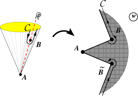
Figure 4: The integration contour $C$ in (2.21). The contour on the cone and its $w$-image are denoted by the same symbol.

Due to the continuity equations, ${\mathfrak{J}}_{1}$ and ${\bar{\mathfrak{J}}}_{1}$ are integrals of motion, i.e., they do not change under continuous deformations of the integration contour.

Finally, let us consider the variation of the on-shell ShG action under an infinitesimal change of the apex angle $\frac{\pi}{\alpha}$. In this case, using the simple electrostatic analogy, one can express $\delta_{\alpha}{\cal A}^{*}$ through the torque applied to the boundary $\partial D_{\epsilon}$

$$\delta_{\alpha}{\cal A}^{*} = \delta\Big{(}\frac{\pi}{\alpha}\Big{)}\ \lim_{\epsilon\to 0}\bigg{[}\,-\int_{\partial D_{\epsilon}}\frac{\mbox{d}\ell}{\pi}\ \epsilon^{\mu\nu}x^{\mu}n^{\sigma}\ T_{\nu\sigma}+\frac{l}{\pi}\ {\hat{\eta}}_{A}+\frac{l^{2}}{\pi}\ \log(\epsilon)\,\bigg{]}\ ,$$ (2.22)

where $x^{1}=\Re e(w-w_{A})$ and $x^{2}=\Im m(w-w_{A})$ are real coordinates on $D_{\epsilon}$, $n^{\sigma}$ is a unit external normal to the boundary $\partial D_{\epsilon}$ and $T_{\mu\nu}=-\frac{1}{4}\ \partial_{\mu}{\hat{\eta}}\partial_{\nu}{\hat{\eta}}+\delta_{\mu\nu}\ \big{[}\,\frac{1}{8}\ \big{(}\partial_{\sigma}{\hat{\eta}})^{2}+2\,\sinh^{2}({\hat{\eta}})\,\big{]}$. The integration contour $\partial D_{\epsilon}$ contains two components $\partial D^{+}_{\epsilon}$ and $\partial D^{-}_{\epsilon}$, related by reflection on the axis $x^{2}=0$. Since each component contributes equally, we replace the integral in (2.22), by $2\int_{\partial D^{+}_{\epsilon}}$ and then evaluate it using the identity

$$4\ \int_{C}\mbox{d}\ell\ \epsilon^{\mu\nu}x^{\mu}n^{\sigma}T_{\nu\sigma}=\int_{C}\mbox{d}x^{\mu}\,\partial_{\mu}\Phi-\int_{C}\mbox{d}\ell\ \partial_{\mu}\big{(}x^{\mu}\Phi)$$ (2.23)

and Eq.(2.19). This yields

$$\alpha^{2}\,\Big{(}\frac{\partial{\cal A}^{*}}{\partial\alpha}\Big{)}_{r,l}=-{\textstyle\frac{1}{2}}\ \Phi_{A}-l\ {\hat{\eta}}_{A}\ ,$$ (2.24)

where ${\hat{\eta}}_{A}$ is given by Eq.(2.9) and $\Phi_{A}$ stands for another “output” constant determined through the solution of the ShG equation – the regularized value of the potential at the apex

$$\Phi_{A}=\lim_{|w-w_{A}|\to 0}\big{(}\,\Phi(w,{\bar{w}})+2l^{2}\,\log|w-w_{A}|\,\big{)}\ .$$ (2.25)

2.3 Generalized FSZ relations

The compatibility of the derived above equations (2.8), (2.20) and (2.24) implies

$$\alpha\,\Big{(}\frac{\partial{\mathfrak{F}}}{\partial l}\Big{)}_{r,\alpha} = -r\,\Big{(}\frac{\partial{\hat{\eta}}_{A}}{\partial r}\Big{)}_{\alpha,l}$$ (2.26)

$$\alpha^{2}\,\Big{(}\frac{\partial{\mathfrak{F}}}{\partial\alpha}\Big{)}_{r,l} = {\textstyle\frac{1}{2}}\ r\,\Big{(}\frac{\partial{\Phi}_{A}}{\partial r}\Big{)}_{\alpha,l}+l\,r\,\Big{(}\frac{\partial{\hat{\eta}}_{A}}{\partial r}\Big{)}_{\alpha,l}\ ,$$

where we introduce the notation

$${\mathfrak{F}}=\frac{r}{2\pi}\ \sin\Big{(}{\frac{\pi}{2\alpha}}\Big{)}\ \big{(}\,{\mathfrak{J}}_{1}+{\bar{\mathfrak{J}}}_{1}\,\big{)}\ .$$ (2.27)

According to Ref.[10] this constant is related to the sine-Gordon $k$-vacuum energy $E_{k}$

$${\mathfrak{F}}=\frac{R}{\pi}\ (\,E_{k}-e_{\infty}\,R\,)\ ,$$ (2.28)

provided $l=2|k|-\frac{1}{2}$, $\alpha=\xi^{-1}$, and $e_{\infty}$ stands for the specific energy of the system with the infinitely large space size [23]:

$$e_{\infty}=\lim_{R\to\infty}\frac{E_{k}}{R}=-\frac{M^{2}}{4}\ \tan\Big{(}\frac{\pi\xi}{2}\Big{)}\ .$$ (2.29)

Thus, for $0<k<\frac{1}{2}$, relations (2.26) are recast into the form

$$\frac{R}{\pi\xi}\ \Big{(}\frac{\partial E_{k}}{\partial k}\Big{)}_{r,\xi}=-r\,\Big{(}\frac{\partial{\hat{\eta}}_{A}}{\partial r}\Big{)}_{\alpha,l}$$ (2.30)

$$\frac{R}{\pi}\ \Big{(}\frac{\partial E_{k}}{\partial\xi}\Big{)}_{r,k}=-\frac{r^{2}}{8\cosh^{2}(\frac{\pi}{2\alpha})}-{\textstyle\frac{1}{2}}\ r\,\Big{(}\frac{\partial{\Phi}_{A}}{\partial r}\Big{)}_{\alpha,l}-l\ r\,\Big{(}\frac{\partial{\hat{\eta}}_{A}}{\partial r}\Big{)}_{\alpha,l}\ .$$

Formulas (2.30) generalize the FSZ relations (1.5) and (1.9) to arbitrary values of the sine-Gordon coupling constant and the quasi-momentum. Indeed, as $\xi=2$, the apex angle of the cone in Fig.2a becomes $2\pi$, whereas $k=\frac{1}{4}$ corresponds to $l=0$, i.e., the solution of the (M)ShG equation remains finite at the tip $A$. In this special case, ${\hat{\eta}}(w,{\bar{w}})$ is expressed in terms of the Painlev${\acute{\rm e}}$ III transcendent (1.7),  (1.8):

$${\hat{\eta}}(w,{\bar{w}})=U\big{(}\,4\,|w-w_{B}|\,\big{)}\ .$$ (2.31)

Since $|w_{A}-w_{B}|=r/4$ (see Fig.2b), the value ${\hat{\eta}}$ at the apex is given by

$${\hat{\eta}}_{A}=U(r)\ ,$$ (2.32)

whereas, as it follows from the general relations $\partial_{w}\partial_{\bar{w}}\Phi=4\ \sinh^{2}({\hat{\eta}})$ and (2.19),

$$r\,\frac{\mbox{d}\Phi_{A}}{\mbox{d}r}=-\int_{r}^{\infty}\mbox{d}t\ t\ \sinh^{2}U(t)\ .$$ (2.33)

2.4 Normalized on-shell action

Although the on-shell action ${\cal A}^{*}$ disappears from the generalized FSZ relations, it is a main player in the derivation of (2.30). Let us discuss some of its properties.

The R.H.S. of (2.28) exponentially decays at $r\to\infty$ (see e.g. [24]). This enables us to represent the on-shell action in the form

$${\cal A}^{*}={\cal A}^{*}_{\infty}+\int_{r}^{\infty}\frac{\mbox{d}r}{r}\ {\mathfrak{F}}\ ,$$ (2.34)

where the integration constant stands for $\lim_{r\to\infty}{\cal A}^{*}$. The calculations outlined in Appendix B yield its explicit form

$${\cal A}^{*}_{\infty} = \log\big{(}3^{\frac{1}{12}}2^{-\frac{2}{9}}\big{)}+(3\xi+1)\ \log\big{(}A_{G}\,2^{-\frac{1}{9}}\,\big{)}$$

$$+ 2\xi k\ \log\Big{(}\frac{4k}{\mbox{e}}\Big{)}+\xi\ \int_{0}^{2k}\mbox{d}x\ \log\left(\,\frac{2^{-2x}\,\Gamma(1-x)}{\Gamma(1+x)}\,\right)\ ,$$

where $A_{G}=1.28243\ldots$ is Glaisher’s constant and we use the sine-Gordon variables $\xi=\alpha^{-1}$ and $k=(2l+1)/4>0$.

The second term in Eq.(2.34) is of primary interest thus we introduce the special notation

$${\mathfrak{Y}}=\int_{R}^{\infty}\frac{\mbox{d}R}{\pi}\ (\,E_{k}-e_{\infty}\,R\,)\ .$$ (2.36)

Evidently it is the on-shell ShG action normalized by the condition

$$\lim_{r\to\infty}{\mathfrak{Y}}=0\ .$$ (2.37)

Then Eqs.(2.8), (2.24) are replaced by

$$\Big{(}\frac{\partial{\mathfrak{Y}}}{\partial k}\Big{)}_{r,\xi} = 2\xi\ \eta_{A}-\Big{(}\frac{\partial{\cal A}_{\infty}^{*}}{\partial k}\Big{)}_{\xi}$$ (2.38)

$$\Big{(}\frac{\partial{\mathfrak{Y}}}{\partial\xi}\Big{)}_{r,k} = {\textstyle\frac{1}{2}}\ \Phi_{A}+l\,\eta_{A}-\Big{(}\frac{\partial{\cal A}_{\infty}^{*}}{\partial\xi}\Big{)}_{k}\ ,$$

where we still assume that $0<k<\frac{1}{2}$.

Using the relation (see the conformal perturbation theory expansion (4.1) bellow)

$$\lim_{R\to 0}RE_{k}=-{\frac{\pi}{6}}\ c_{\rm eff}\ ,$$ (2.39)

where

$$c_{\rm eff}=1-\frac{24\xi k^{2}}{1+\xi}$$ (2.40)

is the “effective” central charge, one can represent ${\mathfrak{Y}}$ in the form which is appropriate for the study of the $R\to 0$ limit,

$${\mathfrak{Y}}={\textstyle\frac{1}{6}}\ c_{\rm eff}\ \log(MR)+{\mathfrak{Y}}_{0}-\frac{(MR)^{2}}{8\pi}\ \tan\Big{(}\frac{\pi\xi}{2}\Big{)}-\int_{0}^{R}\frac{\mbox{d}R}{\pi}\,\left(\,E_{k}+{\frac{\pi c_{\rm eff}}{6R}}\,\right)\ .$$ (2.41)

Here ${\mathfrak{Y}}_{0}$ is some $R$-independent constant. To calculate this constant explicitly one should write ${\mathfrak{Y}}$ as ${\cal A}^{*}-{\cal A}^{*}_{\infty}$, express the functional (2.6) in terms of the original variables of the MShG equation (1.10), and then analyze the limit of a small $r$. The straightforward calculations yield

$${\mathfrak{Y}}_{0} = {\textstyle\frac{1}{12}}\ \log\big{(}\,4\,\xi^{\xi}\,(1+\xi)^{-1-\xi}\,\big{)}-{\textstyle\frac{1}{6}}\ c_{\rm eff}\ \log(r_{\xi})$$

$$- \int_{0}^{\infty}\frac{\mbox{d}x}{x}\ \left(\,\frac{\sinh(x)\cosh(4\xi kx)}{2x\sinh(\xi x)\sinh\big{(}x(1+\xi)\big{)}}-\frac{1}{2\xi(1+\xi)\,x^{2}}+\frac{c_{\rm eff}}{6}\ \mbox{e}^{-2x}\,\right)\,,$$

where $r_{\xi}$ is given by Eq.(1.12).

3 YY-function in the sine-Gordon model

In this section we identify ${\mathfrak{Y}}$ (2.36) with the YY-function and briefly review the approach to numerical calculation of its partial derivatives.

3.1 YY-function for the inhomogeneous 6-vertex model

The sine-Gordon model admits an integrable lattice regularization based on the conventional $R$-matrix of the six-vertex model (see Fig. 5).

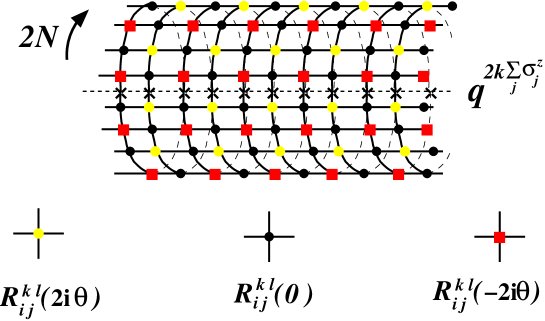
Figure 5: Partition function $Z_{N}={\rm Tr}\big{[}\,q^{k\sum_{j}\sigma_{j}^{z}}\,{\boldsymbol{\tau}}^{N}\,\big{]}$ of the inhomogeneous 6-vertex model on an infinite cylinder. Here ${\boldsymbol{\tau}}$ is the monodromy matrix along the infinite direction and $q=\mbox{e}^{\frac{{\rm i}\pi\xi}{1+\xi}}$. $R_{ij}^{kl}(\lambda)$ are conventional Boltzmann weights for the $6$-vertex model satisfying the Yang-Baxter equation.

Here I shall recall some basic facts concerning the lattice BA equations which are relevant for the purposes of this work. All the details can be found in Refs.[24, 25].

The energy-momentum spectrum in the lattice theory can be calculated by means of the algebraic BA, or Quantum Inverse Scattering Method: BA state is identified by an unordered finite set of distinct, generally complex numbers $\theta_{j}$ which satisfy BA equations

$$\bigg{[}\,\frac{s(\theta_{j}+\Theta+\frac{{\rm i}\pi}{2})\,s(\theta_{j}-\Theta+\frac{{\rm i}\pi}{2})}{s(\theta_{j}+\Theta-\frac{{\rm i}\pi}{2})\,s(\theta_{j}-\Theta-\frac{{\rm i}\pi}{2})}\,\bigg{]}^{N}=-\mbox{e}^{\frac{4{\rm i}\pi\xi k}{1+\xi}}\ \prod_{n}\frac{s(\theta_{j}-\theta_{n}+{\rm i}\pi)}{s(\theta_{j}-\theta_{n}-{\rm i}\pi)}\ ,$$ (3.1)

where

$$s(x)=\sinh\Big{(}\frac{x}{1+\xi}\Big{)}\ ,$$ (3.2)

and $N$ stands for one-half of the number of sites along the compactified direction in Fig. 5. The parameter $\Theta$ controls the world-sheet inhomogeneity of the Boltzmann weights, whereas $k$ in (3.1) is proportional to the twist angle for the quasiperiodic boundary conditions imposed along the compactified direction. Then the energy $E^{(N)}$ and momentum $P^{(N)}$ of the BA state can be extracted from the formulas

$$\exp\Big{(}-{\rm i}\ \frac{E^{(N)}\pm P^{(N)}}{2N}\,\Big{)}=\prod_{j}\frac{s(\frac{{\rm i}\pi}{2}+\Theta\pm\theta_{j})}{s(\frac{{\rm i}\pi}{2}-\Theta\mp\theta_{j})}\ .$$ (3.3)

For the vacuum state all the BA roots are real and their number coincides with $N$, which is assumed to be even bellow. Following Yang and Yang [16], the BA equations in this case can be bring to the form of the extremum condition

$$\frac{\partial Y^{(N)}}{\partial\theta_{j}}=0\ \ \ \ \ \ \ \ \ \ \big{(}\,j=-{\textstyle\frac{N}{2}},\,-{\textstyle\frac{N}{2}}+1,\ldots{\textstyle\frac{N}{2}}-2,\,{\textstyle\frac{N}{2}}-1\,\big{)}$$ (3.4)

for the YY-functional defined by the formulas:

$${Y}^{(N)}=2\ \sum_{j}\Big{(}\,V(\theta_{j})-\frac{2\xi k\,\theta_{j}}{1+\xi}\,\Big{)}+\sum_{j,n}\ U(\theta_{j}-\theta_{n})$$ (3.5)

with

$$V(\theta)=-\frac{N}{\pi}\ \mathchoice{{\vbox{\hbox{$\textstyle-$}}\kern-4.86108pt}}{{\vbox{\hbox{$\scriptstyle-$}}\kern-3.25pt}}{{\vbox{\hbox{$\scriptscriptstyle-$}}\kern-2.29166pt}}{{\vbox{\hbox{$\scriptscriptstyle-$}}\kern-1.875pt}}\!\int_{-\infty}^{\infty}\frac{\mbox{d}\omega}{\omega^{2}}\ \frac{\sinh(\frac{\pi\omega\xi}{2})\,\cos(\omega\Theta)}{\sinh(\frac{\pi\omega(1+\xi)}{2})}\ \mbox{e}^{{\rm i}\omega\theta}$$ (3.6)

and

$$U(\theta)=\frac{1}{\pi}\ \mathchoice{{\vbox{\hbox{$\textstyle-$}}\kern-4.86108pt}}{{\vbox{\hbox{$\scriptstyle-$}}\kern-3.25pt}}{{\vbox{\hbox{$\scriptscriptstyle-$}}\kern-2.29166pt}}{{\vbox{\hbox{$\scriptscriptstyle-$}}\kern-1.875pt}}\!\int_{-\infty}^{\infty}\frac{\mbox{d}\omega}{\omega^{2}}\ \ \frac{\sinh(\frac{\pi\omega\xi}{2})\cosh(\frac{\pi\omega}{2})}{\sinh(\frac{\pi\omega(1+\xi)}{2})}\ \mbox{e}^{{\rm i}\omega\theta}\ .$$ (3.7)

Here and bellow the symbol $\mathchoice{{\vbox{\hbox{$\textstyle-$}}\kern-4.86108pt}}{{\vbox{\hbox{$\scriptstyle-$}}\kern-3.25pt}}{{\vbox{\hbox{$\scriptscriptstyle-$}}\kern-2.29166pt}}{{\vbox{\hbox{$\scriptscriptstyle-$}}\kern-1.875pt}}\!\int$ stands for a principal value integral defined as the half-sum $\frac{1}{2}\,\big{(}\,\int_{-\infty-{\rm i}0}^{+\infty-{\rm i}0}+\int_{-\infty+{\rm i}0}^{+\infty+{\rm i}0}\,\big{)}$.

Eqs.(3.4) can be interpreted as an equilibrium condition for the system of $N$ one-dimensional “electrons” in a presence of confining and linear external potentials. For large separations, $\theta\gg 1$,

$$U(\theta)=-\frac{\xi}{1+\xi}\ |\theta|+O\big{(}\,\mbox{e}^{-\frac{2|\theta|}{1+\xi}}\,\big{)}\ ,$$ (3.8)

therefore the 2-body potential is essentially a 1D repulsive Coulomb potential slightly modified at short distances. Since

$$V(\theta)=\frac{N\xi}{2(1+\xi)}\ |\,\theta-\Theta\,|+\frac{N\xi}{2(1+\xi)}\ |\,\theta+\Theta\,|+O\big{(}\,\mbox{e}^{-\frac{2|\theta\pm\Theta|}{1+\xi}}\,\big{)}\ ,$$ (3.9)

$V(\theta)$ can be interpreted as a potential produced by two heavy positive charges $+\frac{N\xi}{2(1+\xi)}$ placed at $\pm\Theta$. We shall always assume that the external linear potential in (3.5) is sufficiently week and the inequality

$$-{\textstyle\frac{1}{2}}<k<{\textstyle\frac{1}{2}}$$ (3.10)

is fulfilled. For

$$0<\xi<1\ ,$$ (3.11)

the Hessian of the system (3.4), $\frac{\partial^{2}Y_{N}}{\partial\theta_{j}\partial\theta_{n}}$, is positive definite therefore we will focus primarily on this case.

As the physical intuition suggests, the YY-functional (3.5) has a stable minimum at some real distribution of the BA roots

$$\theta^{(N)}_{-\frac{N}{2}}<\theta^{(N)}_{-\frac{N}{2}+1}<\ldots<\theta^{(N)}_{\frac{N}{2}-2}<\theta^{(N)}_{\frac{N}{2}-1}\ .$$ (3.12)

The main subject of our interest is the YY-function, i.e., a critical value of ${Y}^{(N)}$ calculated at this minimum. With some abuse of notations we will denote it by the same symbol as the YY-functional,

$${Y}^{(N)}={Y}^{(N)}(\Theta,\,\xi,\,k)\ .$$ (3.13)

Using the YY-function, the ground state energy (3.3) can be written as

$${E}^{(N)}=\Big{(}\frac{\partial{Y}^{(N)}}{\partial\Theta}\Big{)}_{N,\xi,k}\ ,$$ (3.14)

whereas the momentum associated with the ground state is of course zero.

At large $N$ and finite $\Theta$, the distribution of the BA roots

$$\rho^{(N)}(\theta_{n+\frac{1}{2}})=\frac{1}{N(\theta_{n+1}-\theta_{n})}\ \ \ \ \ \ \ \ \ \ \ \ \big{(}\,\theta_{n+\frac{1}{2}}\equiv{\textstyle\frac{1}{2}}\,(\,\theta_{n+1}+\theta_{n}\,)\,\big{)}$$ (3.15)

is well approximated by the continuous density (see Fig.6)

$$\rho(\theta)=\frac{1}{2\pi}\ \Big{[}\,\frac{1}{\cosh(\theta-\Theta)}+\frac{1}{\cosh(\theta+\Theta)}\,\Big{]}\ .$$ (3.16)

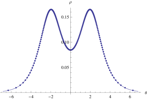
Figure 6: $\rho^{(N)}$ from Eq.(3.15) for $N=400$ and $\Theta=2,\,k=0,\,\xi=\frac{2}{3}.$ The solid line represents the continuous density (3.16).

Therefore the following limit does exist

$$\lim_{N\to\infty\atop\Theta-{\rm fixed}}N^{-2}\,{Y}^{(N)}(\Theta)=y_{\infty}(\Theta)\ ,$$ (3.17)

and it is a simple exercise to show that

$$y_{\infty}(\Theta)=-\frac{1}{\pi}\ \mathchoice{{\vbox{\hbox{$\textstyle-$}}\kern-4.86108pt}}{{\vbox{\hbox{$\scriptstyle-$}}\kern-3.25pt}}{{\vbox{\hbox{$\scriptscriptstyle-$}}\kern-2.29166pt}}{{\vbox{\hbox{$\scriptscriptstyle-$}}\kern-1.875pt}}\!\int_{-\infty}^{\infty}\frac{\mbox{d}\omega}{\omega^{2}}\ \frac{\sinh(\frac{\pi\omega\xi}{2})\ \cos^{2}(\omega\Theta)}{\sinh(\frac{\pi\omega(1+\xi)}{2})\cosh(\frac{\pi\omega}{2})}\ .$$ (3.18)

For large $\Theta$, Eq.(3.18) yields

$$y_{\infty}(\Theta)=\frac{\xi\,|\Theta|}{1+\xi}+\frac{y_{\infty}(0)}{2}+\frac{2}{\pi}\ \mbox{e}^{-2|\Theta|}\ \tan\Big{(}\frac{\pi\xi}{2}\,\Big{)}+O\Big{(}\mbox{e}^{-\frac{4|\Theta|}{1+\xi}}\Big{)}\ .$$ (3.19)

The constant term here coincides with half of the value of (3.18) taken at $\Theta=0$. This is not an accidental relation. Indeed, as $|\Theta|\to+\infty$, all the BA roots split into two clusters centered at $\pm\Theta$. The systems of BA equations for each cluster are completely separated in this limit and reduce to the original form (3.1) with $\Theta=0$ and $N$ is replaced by $N\to N/2$. Hence for any even $N$

$${Y}^{(N)}(\Theta)=\frac{\xi N^{2}}{1+\xi}\ |\Theta|+2\,Y^{({N}/{2})}(0)+o(1)\ \ \ \ \ \ \ {\rm as}\ \ \ \ \Theta\to\pm\infty\ ,$$ (3.20)

where the first term describes monopole-monopole interaction of the “electron” clusters while the second one represents their intrinsic potential energy. Combining (3.14) with (3.20) one also has

$$E^{(N)}(\Theta)-\frac{\xi\,N^{2}}{1+\xi}=o(1)\ \ \ \ \ \ \ {\rm as}\ \ \ \ \Theta\to+\infty\ .$$ (3.21)

It should be emphasized that asymptotic formulas (3.20) and (3.21) do not assume the large-$N$ limit and can be applied for any finite $N$.

3.2 Scaling limit

The sine-Gordon QFT (1.1) manifests itself in the scaling limit when both $N,\,\Theta\to+\infty$ while the scaling parameter

$$r=4\,N\ \mbox{e}^{-\Theta}$$ (3.22)

is kept fixed (RG-invariant). In this case the L.H.S. of (3.21) does not vanish, but has a simple relation to the $k$-vacuum energy [24]:

$$\lim_{N,\Theta\to+\infty\atop r-{\rm fixed}}\ \left(\,{E}^{(N)}-\frac{\xi\,N^{2}}{1+\xi}\ \,\right)=\frac{RE_{k}}{2\pi}+\frac{c_{\rm eff}}{12}\ ,$$ (3.23)

where the effective center charge $c_{\rm eff}$ is given by Eq.(2.40).

In order to study the scaling behavior of the YY-function, it makes sense to consider only the part of the “electron-ion” potential energy corresponding to the mutual interaction of the clusters,

$${Y}_{\rm int}^{(N)}(\Theta)={Y}^{(N)}(\Theta)-\frac{\xi N^{2}}{1+\xi}\ |\Theta|-2\,Y^{(N/2)}(0)\ ,$$ (3.24)

which vanishes as $\Theta\to+\infty$ for any fixed $N$. Taking into account Eqs.(3.14), (3.23), we get

$$\lim_{N,\Theta\to+\infty\atop r-{\rm fixed}}{Y}_{\rm int}^{(N)}(\Theta)=-\int_{0}^{r}\frac{\mbox{d}r}{\pi r}\ \left(\,RE_{k}+{\frac{\pi c_{\rm eff}}{6}}\,\right)\ ,$$ (3.25)

or, equivalently using (2.41),

$$\lim_{N,\Theta\to+\infty\atop r-{\rm fixed}}{Y}_{\rm int}^{(N)}(\Theta)={\mathfrak{Y}}-{\textstyle\frac{1}{6}}\ c_{\rm eff}\ \log(r)+\frac{r^{2}}{8\pi}\ \tan\Big{(}\frac{\pi\xi}{2}\Big{)}-{\mathfrak{Y}}_{0}\ .$$ (3.26)

The last formula allows one to identify the YY-function in the sine-Gordon QFT with the normalized on-shell action ${\mathfrak{Y}}$.

The following comment is in order here. Our analysis is based on the existence of solutions (3.12) of the vacuum BA equations. It can be directly applied to the case $0<\xi<1$ only. At $\xi=1$, the sine-Gordon model is equivalent to the free massive Dirac fermions theory and a closed form of the YY-function can be easily derived from definition (2.36):

$${\mathfrak{Y}}=-r\ \int_{-\infty}^{\infty}\frac{\mbox{d}\tau}{2\pi^{2}}\ \tau\,\sinh(\tau)\,\log\Big{[}\,\big{(}1+\mbox{e}^{-r\cosh(\tau)+2\pi{\rm i}k})(1+\mbox{e}^{-r\cosh(\tau)-2\pi{\rm i}k}\big{)}\,\Big{]}\ .$$ (3.27)

It is expected that for $\xi>1$ the YY-function is uniquely defined through the analytic continuation from the segment $\xi\in(0,1)$.

3.3 BA roots at the large-$N$ limit

Properties of the BA roots at the scaling limit were discussed in Ref. [25]. The roots accumulate at $\theta=\pm\Theta$. However, at the center region (see Fig.6) and at the tails of the distribution the roots remain isolated and their behavior can be described as follows (see Tables 1 and 2 for illustration):

$n$	$N=100$	$N=200$	$N=400$	$N=800$	$N=1600$
$0$	1.04348	1.04342	1.04340	1.04340	1.04340
$1$	3.01807	3.01640	3.01598	3.01588	3.01585
$2$	5.01975	5.01202	5.01009	5.00960	5.00948
$3$	7.03507	7.01378	7.00848	7.00716	7.00683
$4$	9.06565	9.02023	9.00896	9.00615	9.00545
$5$	11.1150	11.0317	11.0111	11.0059	11.0046
$6$	13.1873	13.0489	13.0149	13.0064	13.0043
$7$	15.2870	15.0729	15.0204	15.0074	15.0042
$8$	17.4186	17.1044	17.0280	17.0090	17.0043
$9$	19.5874	19.1447	19.0378	19.0112	19.0046

Table 1: $\frac{r}{2\pi}\ \exp\big{(}\theta^{(N)}_{n}\big{)}$ for $r=1$, $\xi=\frac{2}{3}$ and $k=0$

$n$	$N=100$	$N=200$	$N=400$	$N=800$	$N=1600$
$0$	1.02837	1.02831	1.02830	1.02830	1.028299
$1$	3.01276	3.01111	3.01069	3.01059	3.01056
$2$	5.01652	5.00881	5.00689	5.00641	5.00628
$3$	7.03273	7.01148	7.00619	7.00487	7.00454
$4$	9.06381	9.01843	9.00718	9.00436	9.00366
$5$	11.1135	11.0302	11.0096	11.0045	11.0032
$6$	13.1860	13.0477	13.0136	13.0051	13.0030
$7$	15.2858	15.0718	15.0194	15.0063	15.0031
$8$	17.4176	17.1035	17.0271	17.0081	17.0033
$9$	19.5864	19.1438	19.0369	19.0104	19.0038

Table 2: $\frac{4N}{\pi}\ \exp\big{(}\theta^{(N)}_{n-\frac{N}{2}}+\Theta\big{)}$ for $r=1$, $\xi=\frac{2}{3}$ and $k=0$

• There exist limits

  $$\theta_{j}=\lim_{N,|\Theta|\to\infty\atop r,\,j-{\rm fixed}}\theta_{j}^{(N)}\ \ \ \ \ \ \ \ (\,j=0,\,\pm 1\,\pm 2\ldots\,)$$ (3.28)

  and, for an arbitrary $\Theta\geq 0$,

  $${\tau}^{(+)}_{n} = \lim_{N\to\infty\atop n-{\rm fixed}}\Big{(}\,\theta^{(N)}_{n-\frac{N}{2}}+\log(N)+\Theta\,\Big{)}$$ (3.29)

  $${\tau}^{(-)}_{n} = \lim_{N\to\infty\atop m-{\rm fixed}}\Big{(}\,\theta^{(N)}_{\frac{N}{2}-1-n}-\log(N)-\Theta\,\Big{)}\ \ \ \ \ \ \ \ \ \ \ \ (\,n=0,\,1\ldots\,)\ .$$

• The limiting values of the roots possess the following $n\to+\infty$ asymptotic behavior

  $$\mbox{e}^{\theta_{n}} = \frac{2\pi}{r}\ \big{(}\,2n+1+2k\,\big{)}+O\big{(}n^{-1}\big{)}$$ (3.30)

  $$\mbox{e}^{-\theta_{-n-1}} = \frac{2\pi}{r}\ \big{(}\,2n+1-2k\,\big{)}+O\big{(}n^{-1}\big{)}$$

  and

  $$\exp\big{(}\pm\tau^{(\pm)}_{n}\big{)}=\frac{\pi}{2}\ \big{(}\,2n+1\pm 2k\,\big{)}+O\big{(}n^{-1}\big{)}\ .$$ (3.31)

To probe the infinite sequences $\{\theta_{j}\}_{j=-\infty}^{\infty}$ and $\{\tau^{(\pm)}_{n}\}_{n=0}^{\infty}$ it is useful to consider certain generating functions encoding their properties. Let $\zeta_{+}(\omega)$ and $\zeta_{-}(\omega)$ be functions defined as the analytic continuation of convergent series

$$\zeta_{+}(\omega) = \sum_{n=0}^{\infty}\mbox{e}^{-{\rm i}\omega\theta_{n}}\ \ \ \ \ \ \ \ \ \ \ \Im m(\omega)<-1\ ,$$

$$\zeta_{-}(\omega) = \sum_{n=0}^{\infty}\mbox{e}^{-{\rm i}\omega\theta_{-1-n}}\ \ \ \ \ \ \ \,\Im m(\omega)>1\ .$$ (3.32)

As follows from the asymptotic formulas (3.30), $\zeta_{+}(\omega)\ \big{(}\,\zeta_{-}(\omega)\,\big{)}$ is analytic in the half plane $\Im m(\omega)<1$ $(\Im m(\omega)>-1)$ except at a simple pole at $\omega=-{\rm i}$ $(\omega={\rm i})$ with the residue $-\frac{{\rm i}r}{4\pi}$ $\big{(}\frac{{\rm i}r}{4\pi}\big{)}$. Also note that $\zeta_{\pm}(0)=\mp k$. Therefore

$$\zeta(\omega)=\zeta_{+}(\omega)+\zeta_{-}(\omega)\ ,$$ (3.33)

is an analytic function in the strip $|\Im m(\omega)|<1$ such that

$$\zeta(0)=0\ .$$ (3.34)

In the limit $r\to 0$

$$\zeta(\omega)=\Big{(}\frac{r}{4}\Big{)}^{{\rm i}\omega}\ \big{(}\,\zeta^{\rm(cft)}_{k}(\omega)+o(1)\,\big{)}+\Big{(}\frac{r}{4}\Big{)}^{-{\rm i}\omega}\ \big{(}\,\zeta^{\rm(cft)}_{-k}(-\omega)+o(1)\,\big{)}\ ,$$ (3.35)

where $\zeta^{\rm(cft)}_{\pm k}(\pm\omega)$ are the zeta functions for the sequences $\{\tau^{(\pm)}_{n}\}_{n=0}^{\infty}$ (3.29), i.e.,

$$\zeta^{\rm(cft)}_{\pm k}(\pm\omega)=\sum_{n=0}^{\infty}\exp\big{(}-{\rm i}\omega\tau^{(\pm)}_{n}\,\big{)}\ .$$ (3.36)

The function $\zeta^{\rm(cft)}_{k}(\omega)$ was introduced (in a different overall normalization) and studied in Ref.[26]. Its exhaustive description was found later in Ref.[27] (see also related works [28] and [29]), where it was shown that $\zeta^{\rm(cft)}_{k}(\omega)$ coincides with the zeta function of the Schr${\ddot{\rm o}}$dinger operator

$$-\partial_{x}^{2}+x^{2\alpha}+\frac{l(l+1)}{x^{2}}\ .$$ (3.37)

More precisely, for $0<k<\frac{1}{2}$, the sequences $\big{\{}{\tau}^{(\pm)}_{n}\,\big{\}}_{n=0}^{\infty}$ are simply related to the spectral sets $\big{\{}{\cal E}^{(\pm)}_{n}\}_{n=0}^{\infty}$ of this differential operator:

$$\exp\big{(}\pm{\tau}^{(\pm)}_{n}\big{)}=\frac{\xi r_{\xi}}{8}\ \ \left(\,{\cal E}_{n}^{(\pm)}\,\right)^{\frac{1+\xi}{2}}\ ,$$ (3.38)

with $\alpha=\xi^{-1},\,l=2k-\frac{1}{2}$ and $r_{\xi}$ given by (1.12).

With the above properties of the BA roots it is not difficult to analyze the large $N$-limit of the relation

$$\Big{(}\frac{\partial Y^{(N)}}{\partial k}\Big{)}_{N,\Theta,\xi}=-\frac{4\,\xi}{1+\xi}\ \sum_{j}\theta^{(N)}_{j}\ ,$$ (3.39)

which is derived by differentiating (3.5) with the use of BA equations (3.4). The scaling analog of (3.39) reads

$$\Big{(}\frac{\partial{\mathfrak{Y}}}{\partial k}\Big{)}_{r,\xi}=-\frac{4{\rm i}\,\xi}{1+\xi}\ {\zeta}^{\prime}(0)\ ,$$ (3.40)

where prime stands for the derivative with respect to $\omega$. As follows from (3.35) and $\zeta^{\rm(cft)}_{k}(0)=-k$,

$$\Big{(}\frac{\partial{\mathfrak{Y}}}{\partial k}\Big{)}_{r,\xi}=-\frac{8k\,\xi}{1+\xi}\ \log\Big{(}\frac{r}{4}\Big{)}-\frac{4{\rm i}\,\xi}{1+\xi}\ \left(\,\partial_{\omega}\zeta^{\rm(cft)}_{k}(0)+\partial_{\omega}\zeta^{\rm(cft)}_{-k}(0)\,\right)+o(1)\ \ \ \ \ {\rm as}\ \ \ r\to 0\ .$$ (3.41)

The subleading term of this asymptotic is expressed in terms of the determinant of the differential operator (3.37) and can be calculated explicitly:

$$\Big{(}\frac{\partial{\mathfrak{Y}}}{\partial p}\Big{)}_{r,\xi}=\log\bigg{[}\,\Big{(}\frac{r}{r_{\xi}}\Big{)}^{-\frac{2p}{\xi(1+\xi)}}\ \xi^{\frac{2p}{\xi}}\ (1+\xi)^{-\frac{2p}{1+\xi}}\ \ \frac{\Gamma(1+\frac{p}{\xi})\Gamma(1-\frac{p}{1+\xi})}{\Gamma(1-\frac{p}{\xi})\Gamma(1+\frac{p}{1+\xi})}\,\bigg{]}+o(1)\ \ {\rm as}\ \ r\to 0\,,$$ (3.42)

where we substitute $k$ for the equivalent parameter $p=2\xi k$. Of course, Eq.(3.42) can be alternatively obtained by means of relations (2.41), (2.4). Note the expression in the bracket $\big{[}\,\cdots\,\big{]}$ coincides with Liouville reflection amplitude (analytically continued to the domain $-1<\xi<0$) introduced in the work [30].

3.4 Calculation of partial derivatives of the YY-function

For $0<\xi<1$ the so-called $Q$-function can be defined through the convergent product

$$Q(\theta)={\mathfrak{C}}\ \ \mbox{e}^{\frac{2k\theta}{1+\xi}}\ \prod_{n=0}^{\infty}4\ \mbox{e}^{\frac{\theta_{-n-1}-\theta_{n}}{1+\xi}}\ s\big{(}\theta_{n}-\theta\big{)}\,s\big{(}\theta-\theta_{-n-1}\big{)}\ ,$$ (3.43)

where the abbreviation $s(\theta)$ (3.2) is applied. The $\theta$-independent factor ${\mathfrak{C}}$ can be chosen at will. In what follows it is assumed that

$${\mathfrak{C}}=2^{\frac{1}{1+\xi}}\ \prod_{n=0}^{\infty}\ \exp\Big{[}\,{\textstyle\frac{1}{1+\xi}}\ \big{(}\,2\,\log\big{(}{\textstyle\frac{r}{2\pi(2n+1)}}\big{)}+\theta_{n}-\theta_{-n-1}\,\big{)}\,\Big{]}\ .$$ (3.44)

In the scaling limit, BA equations (3.4) boil down to

$$\epsilon(\theta_{j})=\pi\,(2j+1)\ \ \ \ \ \ (j=0,\,\pm 1,\,\pm 2\ldots\,)\ ,$$ (3.45)

where

$$\epsilon(\theta)={\rm i}\log\left(\,\frac{Q(\theta+{\rm i}\pi\xi)}{Q(\theta-{\rm i}\pi\xi)}\,\right)$$ (3.46)

and the branch of the log is fixed by the condition

$$\epsilon(\theta)=\frac{r\mbox{e}^{\theta}}{2}-2\pi k+o(1)\ \ \ \ \ \ \ \ \ \ {\rm for}\ \ \ \ \ \ \Re e(\theta)\to+\infty\ \ \ \ {\rm and}\ \ \ |\Im m(\theta)|<\frac{\pi}{2}\ .$$ (3.47)

Using the analytic properties of $\zeta_{\pm}(\omega)$ (3.3), definitions (3.43) and (3.46) can be transformed into the integral representations

$$\log Q\big{(}\theta+{\textstyle\frac{{\rm i}\pi(1+\xi)}{2}}\big{)}={\rm i}\pi k+\frac{r\cosh(\theta)}{2\cos(\frac{\pi\xi}{2})}-\frac{1}{2}\ \mathchoice{{\vbox{\hbox{$\textstyle-$}}\kern-4.86108pt}}{{\vbox{\hbox{$\scriptstyle-$}}\kern-3.25pt}}{{\vbox{\hbox{$\scriptscriptstyle-$}}\kern-2.29166pt}}{{\vbox{\hbox{$\scriptscriptstyle-$}}\kern-1.875pt}}\!\int_{-\infty}^{\infty}\frac{\mbox{d}\omega}{\omega}\ \frac{{\zeta}(\omega)}{\sinh(\frac{\pi\omega(1+\xi)}{2})}\ \mbox{e}^{{\rm i}\omega\theta}$$ (3.48)

and

$$\epsilon(\theta)=-2\pi k+r\ \sinh(\theta)-{\rm i}\ \int_{-\infty}^{\infty}\frac{\mbox{d}\omega}{\omega}\ \frac{\sinh(\frac{\pi\omega(1-\xi)}{2})}{\sinh(\frac{\pi\omega(1+\xi)}{2})}\ \zeta(\omega)\ \mbox{e}^{{\rm i}\omega\theta}\ ,$$ (3.49)

respectively. On the other hand, the BA equations (3.45) imply (see Ref.[22] and related Ref.[21] for the original derivation)

$$\zeta(\omega)=\frac{{\rm i}\,\omega\,\sinh(\frac{\pi\omega(1+\xi)}{2})}{\cosh(\frac{\pi\omega}{2})\,\sinh(\frac{\pi\xi\omega}{2})}\ \int_{-\infty}^{\infty}\frac{\mbox{d}\theta}{2\pi}\ \mbox{e}^{-{\rm i}\omega\theta}\,\Im m\Big{[}\,\log\big{(}1+\mbox{e}^{-{\rm i}\epsilon(\theta-{\rm i}0)}\,\big{)}\,\Big{]}\ .$$ (3.50)

Note that at the free-fermion point ($\xi=1$) $\epsilon(\theta)=r\,\sinh(\theta)-2\pi k$, therefore Eq.(3.50) gives

$$\zeta(\omega)=\omega\int_{-\infty}^{\infty}\frac{\mbox{d}\theta}{2\pi}\,\mbox{e}^{-{\rm i}\omega\theta}\Big{[}\,\mbox{e}^{-\frac{\pi\omega}{2}}\ \log\big{(}1+\mbox{e}^{-r\cosh(\theta)+2\pi{\rm i}k}\,\big{)}-\mbox{e}^{\frac{\pi\omega}{2}}\ \log\big{(}1+\mbox{e}^{-r\cosh(\theta)-2\pi{\rm i}k}\,\big{)}\Big{]}.$$ (3.51)

In general, Eqs.(3.49) and (3.50) are combined into a single integral equation on $\epsilon(\theta)$. Once the numerical data for $\epsilon(\theta)$ are available, $\zeta(\omega)$ can be computed by means of (3.50).

Eq.(3.50) shows that $\zeta(\omega)$ is a meromorphic function with simple poles located at $\omega=\pm{\rm i}\,(2n+1)$ and $\omega=\pm\frac{2{\rm i}}{\xi}\ (n+1)\ (n=0,\,1\ldots)$. The residue values are the $k$-vacuum eigenvalues of local and nonlocal integral of motions in the quantum sine-Gordon model [26, 10]. In particular, at the boundary of the strip of analyticity $|\Im m(\omega)|<1$, $\zeta(\omega)$ has simple poles

$$\zeta(\omega)=\mp\frac{\mathfrak{F}}{r}\cot\Big{(}\frac{\pi\xi}{2}\Big{)}\ \frac{{\rm i}}{\omega\pm{\rm i}}+O(1)\ \ \ \ \ {\rm as}\ \ \ \ \omega\to\pm{\rm i}\ ,$$ (3.52)

where ${\mathfrak{F}}$ is given by Eq.(2.28).

This way, the problem of numerical calculation of $k$- and $r$-partial derivatives of the YY-function can be solved by means of relations

$$\Big{(}\frac{\partial{\mathfrak{Y}}}{\partial r}\Big{)}_{\xi,k} = \tan\Big{(}\frac{\pi\xi}{2}\Big{)}\ \lim_{\omega\to\mp{\rm i}}(1\mp{\rm i}\,\omega)\,\zeta(\omega)\ ,$$

$$\Big{(}\frac{\partial{\mathfrak{Y}}}{\partial k}\Big{)}_{r,\xi} = -\frac{4{\rm i}\,\xi}{1+\xi}\ \zeta^{\prime}(0)\ .$$ (3.53)

The calculation of $\xi$-derivative is found out to be a more delicate problem. Rather naive manipulations with the lattice YY-functional (3.5) suggest that

$$\Big{(}\frac{\partial{\mathfrak{Y}}}{\partial\xi}\Big{)}_{r,k} = \frac{1}{4}\ \int_{-\infty}^{\infty}\frac{\mbox{d}\omega}{\omega}\ \frac{\sinh(\pi\omega)}{\sinh^{2}(\frac{\pi\omega(1+\xi)}{2})}\ \zeta(\omega)\,\zeta(-\omega)\ .$$ (3.54)

In Appendix C we present some evidences in support of this relation. Unfortunately it still lacks a rigorous proof.

4 Minisuperspace limit

4.1 Minisuperspace limit of the YY-function

The small-$R$ expansion of the $k$-vacuum energy in the quantum sine-Gordon model was argued in Ref.[7],

$$\frac{RE_{k}}{\pi}=-{\frac{1}{6}}+\frac{4k^{2}\xi}{1+\xi}-\sum_{n=1}^{\infty}\,f_{n}\ r^{\frac{4n}{1+\xi}}\ .$$ (4.1)

The first coefficient $f_{1}$ has a relatively simple explicit form

$$f_{1}=4\ \ \frac{\gamma^{2}(\frac{\xi}{1+\xi})\gamma(\frac{\xi(1-2k)}{1+\xi})\gamma(\frac{\xi(1+2k)}{1+\xi})}{\gamma(\frac{2\xi}{1+\xi})\,(\,(1+\xi)\,r_{\xi}\,)^{{\frac{4}{1+\xi}}}}\ ,$$ (4.2)

where $\gamma(x)=\Gamma(x)/\Gamma(1-x)$ and $r_{\xi}$ (1.12). Let us consider the $\xi\to 0$ limit of (4.1) in which the parameters $r$ and $k$ are kept fixed. One finds

$$\frac{RE_{k}}{\pi}=-\frac{1}{6}+\xi\ a+o(\xi)$$ (4.3)

with

$$a=\nu^{2}+\frac{q^{2}}{2\,(\nu^{2}-1)}+O(q^{4})\ .$$ (4.4)

Here we have denoted

$$q=\Big{(}\frac{r}{4}\Big{)}^{2}\ ,\ \ \ \ \ \ \ \nu=2k\ .$$ (4.5)

In this special (minisuperspace) limit the sine-Gordon QFT reduces to the quantum mechanical problem of particle in the cosine potential whose energy coincides with $a$ from Eq.(4.3). Note that (4.5) are conventional notations in the theory of Mathieu equation [32]. For given $\nu$, $a$ is determined by the Whittaker equation

$$\sin^{2}\Big{(}\frac{\pi\nu}{2}\Big{)}=\Delta_{q}(a)\ \sin^{2}\Big{(}\frac{\pi\sqrt{a}}{2}\Big{)}\ ,$$ (4.6)

where $\Delta_{q}(a)$ is Hill’s determinant

$$\Delta_{q}(a)=\det\begin{pmatrix}&\cdots&\cdots&\cdots&\cdots&\cdots&\cdots&\cdots&\\ &\cdots&\gamma_{-2}&1&\gamma_{2}&\cdots&\cdots&\cdots&\\ &\cdots&\cdots&\gamma_{0}&1&\gamma_{0}&\cdots&\cdots&\\ &\cdots&\cdots&\cdots&\gamma_{2}&1&\gamma_{2}&\cdots&\\ &\cdots&\cdots&\cdots&\cdots&\cdots&\cdots&\cdots&\end{pmatrix}\ ,\ \ \ \ \ \ \ \ \gamma_{2n}=\frac{q}{4n^{2}-a}\ .$$ (4.7)

The solution of Eq.(4.6) is a multivalued function, but the condition (4.4) specifies the proper branch unambiguously. To simplify formulas, we will below treat $a$ as a function of the variables $r$ and $\nu$, i.e.,

$$a=a(r,\nu)\ .$$ (4.8)

Now, using Eqs.(2.41) and (4.3) it is straightforward to obtain the limiting behavior of the YY-function:

$${\mathfrak{Y}}=\frac{1}{6}\ \log\left(\frac{r\xi A_{G}^{12}}{4}\right)+\xi\ \left(\,\frac{1}{4}\,\log\big{(}\,\mbox{e}^{-\frac{1}{3}}\,2^{-\frac{2}{3}}\,\xi\,\big{)}+{\cal Y}(r,\nu)\,\right)+o(\xi)\ ,$$ (4.9)

where

$${\cal Y}(r,\nu) = {\cal Y}_{0}(\nu)-\nu^{2}\ \log\Big{(}\frac{r}{4}\Big{)}-\frac{r^{2}}{16}-\int_{0}^{r}\frac{\mbox{d}t}{t}\ \big{(}\,a(t,\nu)-\nu^{2}\,\big{)}\ ,$$ (4.10)

with

$${\cal Y}_{0}(\nu)=\int_{0}^{\infty}\frac{\mbox{d}x}{x}\ \left(\,\nu^{2}-\frac{\sinh^{2}(\nu x)}{x\sinh(x)}\,\right)\ \mbox{e}^{-x}\ .$$ (4.11)

Note that the above form of ${\cal Y}(r,\nu)$ can be alternatively rewritten as

$${\cal Y}(r,\nu)=\log\big{(}2^{\frac{1}{6}}\,A_{G}^{3}\big{)}+\frac{1}{4}\ \log(r)-\frac{r}{2}+\int_{r}^{\infty}\frac{\mbox{d}t}{t}\ \Big{(}\,a(t,\nu)+\frac{t^{2}}{8}-\frac{t}{2}+\frac{1}{4}\,\Big{)}\ .$$ (4.12)

4.2 Minisuperspace limit of the $Q$-function

The minisuperspace approximation of the $Q$-function at $r=0$ was argued in Appendix B of Ref.[26]. The analysis was based on general properties of the $Q$-function and only minor adjustments are needed to extend it to the case $r>0$.

The $Q$-function is a quasiperiodic solution (see Eq.(3.43))

$$Q\big{(}\theta+{\rm i}\pi(1+\xi)\,\big{)}=\mbox{e}^{2{\rm i}\pi k}\ Q(\theta)$$ (4.13)

of Baxter’s equation (see, e.g., Ref.[10])

$$T_{\frac{1}{2}}(\theta)\,Q(\theta)=Q\big{(}\,\theta+{\rm i}\pi\xi\,\big{)}+Q\big{(}\,\theta-{\rm i}\pi\xi\,\big{)}\ ,$$ (4.14)

where $T_{\frac{1}{2}}(\theta)$ stands for the $k$-vacuum eigenvalue of the transfer matrix. If the overall normalization factor in (3.43) is chosen as in Eq.(3.44), then the $Q$-function also obeys the so-called quantum Wronskian relation

$$Q\big{(}\theta+{\textstyle\frac{{\rm i}\xi\pi}{2}},\,k\,\big{)}\,Q\big{(}\theta-{\textstyle\frac{{\rm i}\xi\pi}{2}},-\,k\,\big{)}-Q\big{(}\theta-{\textstyle\frac{{\rm i}\xi\pi}{2}},\,k\,\big{)}\,Q\big{(}\theta+{\textstyle\frac{{\rm i}\xi\pi}{2}},-\,k\,\big{)}=2{\rm i}\sin(2\pi k)\ ,$$ (4.15)

where we explicitly indicate the dependence on the quasi-momentum. In the minisuperspace limit

$$T_{\frac{1}{2}}(\theta)=2+(\pi\xi)^{2}\ w(\theta)+o(\xi)\ ,$$ (4.16)

whereas Baxter’s equation reduces to the second order differential equation. For the conformal case (i.e., for $r=0$) discussed in [26], $w(\theta)=\mbox{e}^{2\theta}-(2k)^{2}$. Similarly, in the case of finite $r$ one can show that

$$w(\theta)=\frac{r^{2}}{8}\ \cosh(2\theta)-A\ ,$$ (4.17)

with some $\theta$-independent constant $A$ such that

$$\lim_{r\to 0}\,A=(2k)^{2}\ .$$ (4.18)

Thus the minisuperspace limit of the $Q$-function can be described as follows. Let $F_{\nu}(z)$ be Floquet’s solution

$$F_{\nu}(z+{\rm i}\pi)=\mbox{e}^{{\rm i}\pi\nu}\ F_{\nu}(z)\ ,\ \ \ \ \ \ \ \ F_{-\nu}(z)=F_{\nu}(-z)$$ (4.19)

of the modified Mathieu equation

$$-\frac{\mbox{d}^{2}F}{\mbox{d}z^{2}}+\Big{(}\,A-\frac{r^{2}}{8}\,\cosh(2z)\,\Big{)}\,F=0$$ (4.20)

normalized by the condition

$$W[F_{\nu},F_{-\nu}]=-2\ \sin(\pi\nu)\ ,$$ (4.21)

where $W[f,g]$ stands for the Wronskian $fg^{\prime}-gf^{\prime}$. Then, as follows from (4.13)-(4.17),

$$\lim_{\xi\to 0\atop\theta,\,r,\,k-{\rm fixed}}\,\sqrt{\pi\xi}\ Q(\theta,k)=F_{\nu}(\theta)\ \ \ \ \ \ \ \ \ \ {\rm with}\ \ \ \ \ \ \ \ \nu=2k\ .$$ (4.22)

For given $\nu$, the constant $A$ in (4.20) is determined by the quasiperiodicity condition (4.19), which implies the Whittaker equation (4.6) with $a$ replaced by $A$. The extra condition (4.18) enables us to chose the branch of solution of (4.6) unambiguously. Thus we conclude that

$$A=a(r,\nu)\ ,$$ (4.23)

where $a$ is the same function as in Eqs.(4.3), (4.8). It is useful to note that Eq.(4.21) is equivalent to the following normalization condition

$$\int_{0}^{\pi}\mbox{d}y\ F_{\nu}({\rm i}\,y)\,F_{\nu}(-{\rm i}\,y)=2\pi\sin(\pi\nu)\ \bigg{[}\,\Big{(}\frac{\partial a}{\partial\nu}\Big{)}_{r}\,\bigg{]}^{-1}\ .$$ (4.24)

Eq.(4.22) dictates that the BA roots $\{\theta_{j}\}_{j=-\infty}^{\infty}$ (3.28) in the minisuperspace limit turn out to be the zeros of the Mathieu function,

$$\lim_{\xi\to 0\atop j.\,r,\,k-{\rm fixed}}\theta_{j}=z_{j}\ \ \ :\ \ \ F_{\nu}(z_{j})=0\ \ \ \ \ (j=0,\,\pm 1,\pm 2\ldots\,)\ .$$ (4.25)

Using the properties of $F_{\nu}(z)$, it is not difficult to derive the sum rule

$$\Sigma=\sin(\pi\nu)\ \int_{-\infty}^{\infty}\ \frac{\mbox{d}x}{F_{\nu}(x+\frac{{\rm i}\pi}{2})\,F_{\nu}(-x-\frac{{\rm i}\pi}{2})}\ ,$$ (4.26)

where $\Sigma$ stands for the regularized sum of $(-2z_{j})$:

$$\Sigma=2\ \sum_{n=0}^{\infty}\ \Big{(}\,{\frac{\nu}{n+1}}-z_{n}-z_{-n-1}\,\Big{)}-2\nu\ \log\Big{(}\frac{r\mbox{e}^{\gamma_{E}}}{4\pi}\Big{)}$$ (4.27)

($\gamma_{E}$ is Euler’s constant). Note that $\Sigma=-2{\rm i}\,\lim_{r\to 0}\zeta^{\prime}(0)$, and hence Eqs. (3.40), (4.9) imply that

$$\Sigma=\int_{r}^{\infty}\frac{\mbox{d}t}{t}\ \Big{(}\frac{\partial a}{\partial\nu}\Big{)}_{t}\ .$$ (4.28)

4.3 Connection problem for the Painlev${\acute{\bf e}}$ III equation

We now turn to the ShG equation (2.2) at the minisuperspace limit. In this limiting situation the triangle $AB{\tilde{B}}$ in Fig.2b shrinks to a segment while ${\hat{\eta}}$ becomes a certain solution of the Painlev${\acute{\rm e}}$ III equation (1.7)

$$\lim_{\alpha\to\infty\atop r,\,l-{\rm fixed}}{\hat{\eta}}(w,{\bar{w}})=U(4\,|w-w_{A}|)\ \ \ \ \ \ \ \ \ \ \ \ \big{(}\,0<|w-w_{A}|<r/4\,\big{)}\ ,$$ (4.29)

such that

$$\mbox{e}^{2U(t)}=\kappa^{2}\ t^{4\nu-2}+o(t^{4\nu-2})\ \ \ \ \ \ \ {\rm for}\ \ \ \ \ t\to 0\ .$$ (4.30)

Parameters $\nu$ and $\kappa$ are related to $l$ and $\eta_{A}$ (2.9) as follows

$$\nu = l+{\textstyle\frac{1}{2}}$$ (4.31)

$$\log\kappa = -l\,\log(4)+\lim_{\alpha\to\infty\atop l,\,r-{\rm fixed}}\eta_{A}\ .$$

Let us discuss the solution satisfying (4.30) in the context of the general theory of Painlev${\acute{\rm e}}$ III equation. For $0<\nu<1$ and real $\kappa$, the asymptotic condition (4.30) unambiguously specifies a two-parameter family of real solutions of the Painlev${\acute{\rm e}}$ III equation. A systematic small-$t$ expansion of (4.30) has the form of the double series [7]

$$\mbox{e}^{2U(t)}=\kappa^{2}\ t^{4\nu-2}+\sum_{m,n=0\atop m+n>1}^{\infty}\ B_{m,n}\ t^{4(1-\nu)m+4\nu n-2}$$ (4.32)

whose coefficients are uniquely determined through the parameters $\nu$ and $\kappa$ by a recursion relation which follows from the differential equation (1.7).

The expansion (4.32) is expected to converge for sufficiently small $t$. Let $t=r$ be the closest singularity to the origin. The differential equation (1.7) possesses the Painlev${\acute{\rm e}}$ property which states that, except at $t=0$ and $t=\infty$, the only possible singularities of $\mbox{e}^{2U}$ are the second order poles of the form $\mbox{e}^{2U(t)}=\frac{4}{(t-r)^{2}}-\frac{4}{r\,(t-r)}+C+o(1)$ with some constant $C$. Further terms in this Laurent expansion are expressed in terms of $r$ and $C$. They can be easily generated through the differential equation (1.7). It will be convenient for us to substitute $C$ for an equivalent parameter $c$ such that

$$\mbox{e}^{2U(t)}=\frac{4}{(t-r)^{2}}-\frac{4}{r\,(t-r)}+\frac{13-16\,c}{3\,r^{2}}+\frac{2\,(16\,c-7)}{3\,r^{3}}\ (t-r)+O\big{(}(t-r)^{2}\big{)}\ .$$ (4.33)

We will focus on the case when the closest pole to the origin is located at the positive real axis, i.e., $r>0$. This requirement imposes certain constraints on admissible values of $\kappa$ and $c$. Within the admissible domains, each pair $(\nu,\kappa)$ or $(r,c)$ can serve as an independent set of parameters for the two-parameter family of real solutions of the Painlev${\acute{\rm e}}$ III equation which are regular at the segment $t\in(0,r)$ and characterized by the behaviour $U\to(2\nu-1)\,\log(t)+O(1)$ as $t\to 0$; However, it is more convenient to choose $(r,\nu)$ with $r>0$, $0<\nu<1$, as a basic set of independent parameters.

At this point, we turn to the problem of finding the functions $\kappa=\kappa(r,\nu)$ and $c=c(r,\nu)$, i.e., the connection problem for the local expansions (4.32) and (4.33). It is relatively easy to establish the relation

$$\Big{(}\frac{\partial c}{\partial\nu}\Big{)}_{r}=-r\,\Big{(}\frac{\partial\log\kappa}{\partial r}\Big{)}_{\nu}\ .$$ (4.34)

The proof is similar to our previous derivation of the generalized FSZ relations; One should consider the action functional

$${\cal S}[U]=\frac{1}{4}\lim_{\epsilon\to 0}\bigg{[}\int_{\epsilon}^{r}\mbox{d}t\,t\Big{(}{\dot{U}}^{2}+\sinh^{2}(U)-\frac{2}{(r-t)^{2}}\Big{)}+2(2\nu-1)\,U(\epsilon)-(2\nu-1)^{2}\log(\epsilon)\bigg{]}$$ (4.35)

where the dot stands for the $t$-derivative. For $U(t)$, $t\in(0,r)$ satisfying the boundary conditions (4.30), (4.33), the functional ${\cal S}[U]$ is well defined and its variation vanishes provided $U(t)$ satisfies the Painlev${\acute{\rm e}}$ III equation and $\delta U(r)=0$. Let ${\cal S}^{*}$ be the on-shell value of (4.35). One can show that

$$r\,\Big{(}\frac{\partial{\cal S}^{*}}{\partial r}\Big{)}_{\nu} = \frac{1}{4}-\frac{r^{2}}{8}-c$$ (4.36)

$$\Big{(}\frac{\partial{\cal S}^{*}}{\partial\nu}\Big{)}_{r} = \log\kappa\ ,$$

and the compatibility of these equations implies (4.34).

Now let us apply the results of the previous sections. At the minisuperspace limit the first generalized FSZ relation (2.30) yields the formula identical to (4.34) with $c(r,\nu)$ replaced by $a(r,\nu)$. Therefore, we conclude that $c-a$ does not depend on $\nu$. It is straightforward to analyze $r\to 0$ behaviour of the on-shell action:

$${\cal S}^{*}=\Big{(}\,\frac{1}{4}-\nu^{2}\,\Big{)}\ \log(r)+\nu\log\Big{(}\frac{8\nu}{\mbox{e}}\Big{)}-\frac{1}{4}\ \log\Big{(}\frac{4}{\mbox{e}}\Big{)}-\frac{r^{2}}{16}+O(r^{4})\ .$$ (4.37)

This asymptotic formula, combined with (4.36), implies that $c=\nu^{2}+O(r^{4})$, and hence $c-a=O(r^{4})$ (see Eq.(4.4)). In Appendix D it is explained how to systematically recover the small-$r$ expansion of $c(r,\nu)$. The calculations yield the expansion

$$c = \nu^{2}+\frac{1}{2\,(\nu^{2}-1)}\ \Big{(}\frac{r}{4}\Big{)}^{4}+\frac{5\,\nu^{2}+7}{32\,(\nu^{2}-1)^{3}\,(\nu^{2}-4)}\ \Big{(}\frac{r}{4}\Big{)}^{8}$$

$$+ \frac{9\,\nu^{4}+58\,\nu^{2}+29}{64\,(\nu^{2}-1)^{5}\,(\nu^{2}-4)\,(\nu^{2}-9)}\ \Big{(}\frac{r}{4}\Big{)}^{12}+O(r^{16})\ ,$$

which matches exactly the small-$r$ expansion of $a(r,\nu)$ (see Eq.(4.4) and formula 20.3.15 in Ref.[32]). The formal derivation of the relation

$$c=a(r,\,\nu)$$ (4.39)

can be obtained with the use of equations (A.3), (A.17) from Appendix A, combined with the results from Section 4.2. Eq.(4.39), together with

$$\kappa = 8\nu\ r^{-2\nu}\ \exp\bigg{[}\,\int_{0}^{r}\frac{\mbox{d}t}{t}\ \bigg{(}\,2\nu-\Big{(}\frac{\partial a}{\partial\nu}\Big{)}_{t}\,\bigg{)}\,\bigg{]}$$

$$= 8^{1-2\nu}\ \ \frac{\Gamma(1-\nu)}{\Gamma(\nu)}\ \exp\bigg{[}\,\int_{r}^{\infty}\frac{\mbox{d}t}{t}\ \Big{(}\frac{\partial a}{\partial\nu}\Big{)}_{t}\,\bigg{]}\ ,$$

leads to an explicit solution of the connection problem for local expansions (4.32) and (4.33). The domain of applicability of Eqs.(4.39), (4.3) is given by the inequalities (see Fig. 7a)

$$0<\nu<1\ ,\ \ \ \ \ \ \ \kappa>8^{1-2\nu}\ \ \frac{\Gamma(1-\nu)}{\Gamma(\nu)}\ .$$ (4.41)

It can be equivalently described in terms of the pair $(r,c)$:

$$r>0\ ,\ \ \ \ \ \ \ \ \ \ a_{0}(r)<c<b_{1}(r)\ ,$$ (4.42)

where $a_{0}=a(r,0)$ and $b_{1}=\lim_{\nu\to 1}a(r,\nu)$ stand for the minimum and maximum of the first conduction band for the Mathieu equation, respectively (see Fig. 7b).

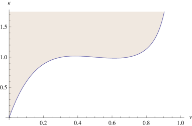
$(a)$            (b)  

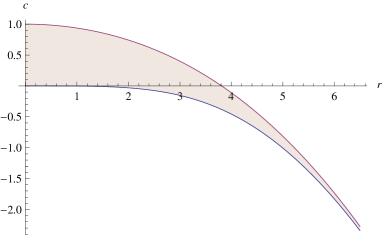
Figure 7: The admissible parameter domain for the two-parameter family of solutions of the Painlev${\acute{\rm e}}$ III equation: $(a)$ in terms of $(\nu,\kappa)$ from (4.30). $(b)$ in terms of $(r,c)$ from (4.33).

Finally, let us briefly discuss the minisuperspace limit for $\Phi^{(-)}=\frac{1}{2}\,(\,\Phi-{\hat{\eta}})$. Contrary to ${\hat{\eta}}(w,{\bar{w}})$, the potential $\Phi(w,{\bar{w}})$ does not have a finite limit for $0<|w-w_{A}|<r/4$. However, the divergent part of $\Phi^{(-)}(w,{\bar{w}})$ for $0<|w-w_{A}|<r/4$ is somewhat trivial and can be resolved by by means of the decomposition (A.13) from Appendix A. The non-trivial part ${\tilde{\Phi}}^{(-)}$ is specified by the conditions (A.14),(A.15) and remains finite as $\alpha\to\infty$. It is convenient to introduce

$$W(t)=-l(l+1)\ \log|w-w_{A}|+\lim_{\alpha\to\infty\atop r,\,l-{\rm fixed}}{\tilde{\Phi}}^{(-)}(w,{\bar{w}})\ ,$$ (4.43)

where $t=4\,|w-w_{A}|<r$ and $l=\nu-\frac{1}{2}$. As follows from Eqs.(A.2),  (A.13), $W(t)$ satisfies the linear inhomogeneous differential equation (assuming $U$ is given)

$$\frac{4}{t}\ \frac{\mbox{d}}{\mbox{d}t}\Big{(}\,t\,\frac{\mbox{d}W}{\mbox{d}t}\,\Big{)}=\mbox{e}^{-2U(t)}-1\ ,$$ (4.44)

and the boundary condition

$$W(t)=\Big{(}\,\frac{1}{4}-\nu^{2}\,\Big{)}\ \log\Big{(}\frac{t}{4}\Big{)}+o(1)\ ,\ \ \ {\rm as}\ \ \ \ \ t\to 0\ .$$ (4.45)

Therefore

$$W(t)=\Big{(}\,\frac{1}{4}-\nu^{2}\,\Big{)}\ \log\Big{(}\frac{t}{4}\Big{)}-\frac{t^{2}}{16}-\frac{1}{4}\ \int_{0}^{t}\mbox{d}\tau\,\tau\,\log\Big{(}\frac{\tau}{t}\Big{)}\ \mbox{e}^{-2U(\tau)}\ .$$ (4.46)

The $t$-derivative of ${W}(t)$ at $t=r$ is given by

$$r\,{\dot{W}}(r)=\frac{1}{4}-\frac{r^{2}}{8}-\nu^{2}+\frac{1}{4}\ \int_{0}^{r}\mbox{d}t\,t\,\mbox{e}^{-2U(t)}$$ (4.47)

and it is not difficult to show that

$${\dot{W}}(r)=\Big{(}\frac{\partial{\cal S}^{*}}{\partial r}\Big{)}_{\nu}\ .$$ (4.48)

The last two relations combined with Eqs.(4.36), (4.39) imply

$$\frac{1}{4}\ \int_{0}^{r}\mbox{d}t\,t\,\mbox{e}^{-2U(t)}=\nu^{2}-a(r,\nu)\ .$$ (4.49)

By transforming the integrals as in Ref.[35], the value of $W(t)$ at $t=r$ can be expressed in terms of $a$, $\kappa$ and ${\cal S}^{*}$:

$$W(r)=\frac{1}{2}\ \log\Big{(}\frac{r}{4}\Big{)}-\frac{r^{2}}{8}+\Big{(}\nu-\frac{1}{2}\Big{)}^{2}+2\nu^{2}\,\log(2)-a+\nu\ \log(\kappa)-{\cal S}^{*}\ ,$$ (4.50)

which is equivalent to the following relations

$$W(r)=\Big{(}\,\frac{1}{4}-\nu^{2}\,\Big{)}\,\log\Big{(}\frac{r}{4}\Big{)}-\frac{r^{2}}{16}-\int_{0}^{r}\frac{\mbox{d}t}{t}\,\bigg{(}\,t\,\Big{(}\frac{\partial a}{\partial t}\Big{)}_{\nu}+\nu\,\Big{(}\frac{\partial a}{\partial\nu}\Big{)}_{t}-a(t,\nu)-\nu^{2}\,\bigg{)}\ ,$$ (4.51)

or

$$W(r) = {\cal Y}_{0}(\nu)-\log\bigg{[}\,A_{G}^{3}\ \ \ \mbox{e}^{-\frac{1}{4}-\nu^{2}}\ 2^{2\nu^{2}+\frac{2}{3}}\ \bigg{(}\,\frac{\Gamma(1+\nu)}{\Gamma(1-\nu)}\,\bigg{)}^{\nu}\,\bigg{]}$$

$$+ \int_{r}^{\infty}\frac{\mbox{d}t}{t}\ \bigg{(}\,t\,\Big{(}\frac{\partial a}{\partial t}\Big{)}_{\nu}+\nu\,\Big{(}\frac{\partial a}{\partial\nu}\Big{)}_{t}-a(t,\nu)+\frac{t^{2}}{8}-\frac{1}{4}\,\bigg{)}\ ,$$

where ${\cal Y}_{0}(\nu)$ is given by Eq.(4.11). Note that the last term in Eq.(4.3) vanishes as $r\to\infty$ while the remaining part reproduces the result quoted in Ref.[7].

5 Concluding remark

In this work we have described the link between the action functional for the classical ShG equation and the YY-function corresponding to the $k$-vacuum states in the quantum sine-Gordon model. The natural question arises: Can this relation be generalized for the excited states? Nowadays the machinery of the Destri de Vega equation for the excited states are well developed [25, 36], so that the calculation of the YY-function for the excited states does not seem to be a particularly complicated problem. However, it remains unclear how to construct integrable classical equations associated with the excited states and perhaps more importantly, what all of this really means.

Appendix A Appendix: Basic properties of the potential $\Phi$

Let us define the following linear combinations of the solution ${\hat{\eta}}$ of the ShG equation (2.2) and the potential $\Phi$ (2.14)

$$\Phi^{(\pm)}={\textstyle\frac{1}{2}}\ \big{(}\,\Phi\pm{\hat{\eta}}\,\big{)}\ .$$ (A.1)

They satisfy the relations

$$\partial^{2}_{w}\Phi^{(\pm)}={\textstyle\frac{1}{2}}\ \big{(}\,(\partial_{w}{\hat{\eta}})^{2}\pm\partial^{2}_{w}{\hat{\eta}}\,\big{)}\,,\ \ \ \partial^{2}_{\bar{w}}\Phi^{(\pm)}={\textstyle\frac{1}{2}}\ \big{(}\,(\partial_{\bar{w}}{\hat{\eta}})^{2}\pm\partial^{2}_{\bar{w}}{\hat{\eta}}\,\big{)}\ ,\ \ \ \ \partial_{w}\partial_{\bar{w}}\Phi^{(+)}=\mbox{e}^{\pm 2{\hat{\eta}}}-1\,,$$ (A.2)

which can be considered as a closed system of nonlinear partial differential equations. Results of Refs.[7] and [10] imply that the desirable solution of (A.2) is expressed in terms of the Fredholm determinants

$$\Phi^{(\pm)}(w,{\bar{w}})=\log\det\bigg{(}\,{\mathbb{I}}\pm\frac{{\mathbb{K}}_{w,{\bar{w}}}}{4\pi}\,\bigg{)}\ .$$ (A.3)

The kernel of the integral operator ${\mathbb{K}}_{w,{\bar{w}}}$ reads

$$K_{w,{\bar{w}}}(\theta,\theta^{\prime}) = \frac{\sqrt{g_{w,{\bar{w}}}(\theta)g_{w,{\bar{w}}}(\theta^{\prime})}}{\cosh\big{(}\frac{\theta-\theta^{\prime}}{2}\big{)}}\ ,$$ (A.4)

$$g_{w,{\bar{w}}}(\theta) = T_{\frac{1}{2}}\big{(}\theta+{\textstyle\frac{{\rm i}\pi(\alpha+1)}{2\alpha}}\big{)}\ \exp\big{(}-2w\,\mbox{e}^{\theta}-2{\bar{w}}\,\mbox{e}^{-\theta}\,\big{)}\ ,$$

where $T_{\frac{1}{2}}(\theta)$ is defined by the $Q$-function (3.43) through Baxter’s equation (4.14) with $\xi=\alpha^{-1}$. In (A.3) $(w,{\bar{w}})$ play a r${\hat{\rm o}}$le of complex parameters. Within the domain

$$|\arg(w)|\leq{\textstyle\frac{\pi(\alpha+1)}{2\alpha}}\ ,$$ (A.5)

$\Phi^{(\pm)}(w,{\bar{w}})$ can be represented by convergent series

$$\Phi^{(\pm)}(w,{\bar{w}})=\sum_{n=1}^{\infty}\frac{(\pm 1)^{n}}{n}\ \Phi_{n}(w,{\bar{w}})\ ,$$ (A.6)

$$\Phi_{n}(w,{\bar{w}})=\int_{-\infty}^{\infty}\prod_{j=1}^{n}\left(\,\frac{\mbox{d}\theta_{j}}{4\pi}\ \frac{g_{w,{\bar{w}}}(\theta_{j})}{\cosh\big{(}\frac{\theta_{j}-\theta_{j+1}}{2}\big{)}}\,\right)\ ,$$

where it is implied that $\theta_{n+1}\equiv\theta_{1}$. Some immediate consequences of (A.6),

$$\Phi^{(\pm)}\big{(}w\,\mbox{e}^{\frac{{\rm i}\pi(\alpha+1)}{\alpha}},\,{\bar{w}}\,\mbox{e}^{-\frac{{\rm i}\pi(\alpha+1)}{\alpha}}\,\big{)} = \Phi^{(\pm)}(w,\,{\bar{w})}\ \ \ \ \ \ \ \ {\rm for}\ \ \ \ \ |w|>|w_{B}|$$ (A.7)

and

$$\lim_{|w|\to\infty}\Phi^{(\pm)}(w,{\bar{w}})=0\ ,$$ (A.8)

have been used in the derivation of basic Eq.(2.20). By deforming the integration contours in (A.6), the applicable domain (A.5) can be slightly extended to the triangle $OB{\tilde{B}}$ (see Fig.2b). This leads to the fact that for $\Re e(w-w_{B})\geq 0$

$$\Phi^{(\pm)}(w,{\bar{w}})=\Phi^{(\pm)}({\bar{w}},w)\ .$$ (A.9)

Yet the expansions (A.6) cannot be applied inside the triangle $AB{\tilde{B}}$,

$$0<\Re e(w-w_{A})<\Re e(w_{B}-w_{A})\,,\ \ \ \ \ \ \ \arg(w-w_{A})<\frac{\pi}{2\alpha}\ .$$ (A.10)

Within this domain, ${\hat{\eta}}(w,{\bar{w}})$ satisfies the symmetry relations

$${\hat{\eta}}\big{(}w_{A}+(w-w_{A})\,\mbox{e}^{\frac{{\rm i}\pi}{\alpha}},\,{\bar{w}}_{A}+({\bar{w}}-{\bar{w}}_{A})\,\mbox{e}^{-\frac{{\rm i}\pi}{\alpha}}\,\big{)}={\hat{\eta}}(w,\,{\bar{w}})={\hat{\eta}}({\bar{w}},\,w)\ ,$$ (A.11)

whereas, as follows from (A.2),

$$\partial_{w}^{2}\,\delta\Phi^{(\pm)}=\partial_{\bar{w}}^{2}\,\delta\Phi^{(\pm)}=\partial_{w}\partial_{\bar{w}}\,\delta\Phi^{(\pm)}=0\ ,$$ (A.12)

where $\delta\Phi^{(\pm)}=\Phi^{(\pm)}\big{(}w_{A}+(w-w_{A})\,\mbox{e}^{\frac{{\rm i}\pi}{\alpha}},\,{\bar{w}}_{A}+({\bar{w}}-{\bar{w}}_{A})\,\mbox{e}^{-\frac{{\rm i}\pi}{\alpha}}\,\big{)}-\Phi^{(\pm)}(w,\,{\bar{w}})$. From Eqs.(2.4), (A.12) and the reflection symmetry relation (A.9) applied to the segment $B{\tilde{B}}$, we deduce that within the domain (A.10) $\Phi^{\pm}$ can be written in the form

$$\Phi^{(\pm)}(w,{\bar{w}})=-l(l\mp 1)\,\log|w-w_{A}|+(w-w_{A})\,{\bar{J}}+({\bar{w}}-{\bar{w}}_{A})\,J+\Phi^{(\pm)}_{A}+{\tilde{\Phi}}^{\pm}(w,{\bar{w}})\,,$$ (A.13)

where $\Phi^{(\pm)}_{A}$ and $J={\bar{J}}$ are some real constants,

$${\tilde{\Phi}}^{(\pm)}\big{(}w_{A}+(w-w_{A})\,\mbox{e}^{\frac{{\rm i}\pi}{\alpha}},\,{\bar{w}}_{A}+({\bar{w}}-{\bar{w}}_{A})\,\mbox{e}^{-\frac{{\rm i}\pi}{\alpha}}\,\big{)}={\tilde{\Phi}}^{\pm}(w,\,{\bar{w}})={\tilde{\Phi}}^{\pm}({\bar{w}},\,w)$$ (A.14)

and

$$\lim_{|w-w_{A}|\to 0}{\tilde{\Phi}}^{(\pm)}(w,{\bar{w}})=0\ .$$ (A.15)

The constants $\Phi^{(\pm)}_{A}$ in (A.13) are given by the linear combinations of ${\hat{\eta}}_{A}$ (2.9) and $\Phi_{A}$ (2.25):

$$\Phi_{A}^{(\pm)}={\textstyle\frac{1}{2}}\,(\,\Phi_{A}\pm\eta_{A}\,)\ .$$ (A.16)

As for $J$ and ${\bar{J}}$, the calculations performed in Section 2.2 imply that

$$\int_{D}{\frac{{\mbox{d}w}\wedge{\mbox{d}}{\bar{w}}}{2\pi{\rm i}}}\ \ 4\,\big{(}\,\mbox{e}^{\pm 2{\hat{\eta}}}-1\,\big{)}=\frac{l(l\mp 1)}{\alpha}\pm\frac{1}{2}+\frac{1}{12}-\frac{r}{2\pi}\ \sin\Big{(}{\frac{\pi}{2\alpha}}\Big{)}\ \big{(}\,{\mathfrak{J}}_{1}+{\bar{\mathfrak{J}}}_{1}\,\big{)}\ .$$ (A.17)

On the other hand, the integrand here coincides with the Laplacian $4\,\partial_{w}\partial_{\bar{w}}\Phi^{(\pm)}$, and the L.H.S. of (A.17) can be expressed in terms of $J={\bar{J}}$. This yields the relations

$$J={\mathfrak{J}}_{1}\ ,\ \ \ \ \ \ \ \ \ \ \ \ \ {\bar{J}}={\bar{\mathfrak{J}}}_{1}\ .$$ (A.18)

Finally, note that Eqs.(2.5), (A.2) yield the following asymptotic behaviours in the vicinity of $B\sim{\tilde{B}}$ (see Fig. 2b)

$${\Phi}^{(+)}\to-\frac{7}{36}\ \log|w-w_{B}|+O(1)\ ,\ \ \ \ \ \ \ \ \ {\Phi}^{(-)}\to\frac{5}{36}\ \log|w-w_{{\tilde{B}}}|+O(1)\ .$$ (A.19)

Appendix B Appendix: Calculation of ${\cal A}^{*}_{\infty}=\lim_{r\to\infty}{\cal A}^{*}$

For large $r$ the dominating contributions to the on-shell action (2.6) come from the vicinities of the points $A$ and $B\sim{\tilde{B}}$ (see Fig.2b). Near these points, ${\hat{\eta}}$ can be approximated by $U(4|w-w_{A}|)|_{\nu=l+\frac{1}{2}}$ and $U(4|w-w_{B}|)|_{\nu=\frac{1}{3}}$, respectively, where $U$ are the Painlev${\acute{\rm e}}$ III transcendents, i.e., regular at $t>0$ solutions of Eq.(1.7) satisfying the boundary conditions

$$U\to\begin{cases}&(2\nu-1)\ \log\big{(}\frac{t}{4}\big{)}+U_{0}(\nu)+o(1)\ ,\ \ \ \ {\rm as}\ \ \ \ t\to 0\\ &0\ ,\ \ \ \ \ \ \ \ \ \ \ \ \ \ \ \ \ \ \ \ \ \ \ \ \ \ \ \ \ \ \ \ \ \ \qquad\ \ \ \ {\rm as}\ \ \ \ t\to\infty\end{cases}\ .$$

This observation implies that the limiting value of the on-shell action (2.6) is given by

$${\cal A}^{*}_{\infty}=3\ {\cal S}^{*}_{\infty}\big{(}{\textstyle{\frac{1}{3}}}\big{)}+\alpha^{-1}\ {\cal S}^{*}_{\infty}(\nu)\ ,$$ (B.1)

where ${\cal S}^{*}_{\infty}(\nu)$ is the on-shell value of the action functional for the Painlev${\acute{\rm e}}$ III equation,

$${\cal S}_{\infty}[U]=\frac{1}{4}\ \lim_{\epsilon\to 0}\ \bigg{[}\,\int_{\epsilon}^{\infty}\mbox{d}t\ t\ \big{(}\,{\dot{U}}^{2}+\sinh^{2}(U)\,\big{)}+2\,(2\nu-1)\ U(\epsilon)-(2\nu-1)^{2}\ \log\Big{(}\frac{\epsilon}{4}\Big{)}\,\bigg{]}\,.$$ (B.2)

Here the dot stands for the $t$-derivative. Varying (B.2) with respect to $\nu$ yields equation $U_{0}(\nu)=\frac{{\rm d}{\cal S}^{*}_{\infty}}{{\rm d}\nu}$. Since ${\cal S}^{*}_{\infty}(\frac{1}{2})=0$, one has

$${\cal S}^{*}_{\infty}(\nu)=\int_{\frac{1}{2}}^{\nu}\mbox{d}x\ U_{0}(x)\ .$$ (B.3)

An explicit form of $U_{0}(\nu)$ is well known [6],

$$U_{0}=\log\left(\,2^{1-2\nu}\,\frac{\Gamma(1-\nu)}{\Gamma(\nu)}\,\right)\ .$$ (B.4)

Combining (B.1), (B.3) with (B.4) one arrives to (2.4).

Appendix C Appendix: Formula for $\big{(}\frac{\partial{\mathfrak{Y}}}{\partial\xi}\big{)}_{r,k}$

This section presents some supporting evidences for relation (3.54) which is expected to hold for any $\xi>0$.

Using Eqs.(3.49), (3.50) and (3.4) it is easy to show that for $\xi\geq 1$ (i.e., in the case without soliton-antisoliton bound states) the large-$r$ behaviour of ${\mathfrak{Y}}$ is given by

$${\mathfrak{Y}}(r)=-\frac{2}{\pi^{2}}\ \cos(2\pi k)\ K_{0}(r)+O(\mbox{e}^{-2r})\ ,$$ (C.1)

whereas

$$\zeta(\omega)=-\frac{\omega\,\sinh(\frac{\pi\omega(1+\xi)}{2})}{\pi\,\cosh(\frac{\pi\omega}{2})\,\sinh(\frac{\pi\xi\omega}{2})}\ \cosh\Big{(}\,\frac{\pi\omega}{2}-2\pi{\rm i}k\Big{)}\ K_{{\rm i}\omega}(r)+O(\mbox{e}^{-2r})\ .$$ (C.2)

Here $K_{\nu}(r)$ is the modified Bessel function and the symbol $O(\mbox{e}^{-2r})$ stands for an asymptotic behaviour of the form $\propto r^{\gamma}\,\mbox{e}^{-2r}$ as $r\to\infty$ with some exponent $\gamma$. The leading large-$r$ asymptotic of ${\mathfrak{Y}}$ does not depend on $\xi$ and hence the L.H.S. of (3.54) decays as $O(\mbox{e}^{-2r})$. Thus Eq.(3.54) is qualitatively consistent with asymptotics (C.1) and (C.2). A quantitative comparison can be made for $\xi=2$ and $k=\pm\frac{1}{4}$. In this case [7]

$$\Big{(}\frac{\partial{\mathfrak{Y}}}{\partial\xi}\Big{)}_{r,k}=\frac{1}{2\pi^{2}}\ \int_{r}^{\infty}\mbox{d}t\ t\,\log\Big{(}\frac{t}{r}\Big{)}\,K_{0}^{2}(t)+O(\mbox{e}^{-4r})\$$ (C.3)

(This formula follows immediately from (1.9) and the large-$t$ asymptotic $U(t)=\frac{1}{\pi}\,K_{0}(t)+O(\mbox{e}^{-2t})$), so that Eq.(3.54) implies the following easily established identity

$$\int_{r}^{\infty}\mbox{d}t\ t\,\log\Big{(}\frac{t}{r}\Big{)}\,K_{0}^{2}(t)=\int_{-\infty}^{\infty}\mbox{d}\omega\ \,\frac{\omega\ K^{2}_{{\rm i}\omega}(r)}{2\sinh(\pi\omega)}\ .$$ (C.4)

Another piece of evidence supporting (3.54) comes from the consideration of $r\to 0$ limit. Using Eq.(3.35) one finds

$$\frac{1}{4}\ \int_{-\infty}^{\infty}\frac{\mbox{d}\omega}{\omega}\ \frac{\sinh(\pi\omega)}{\sinh^{2}(\frac{\pi\omega(1+\xi)}{2})}\ \zeta(\omega)\,\zeta(-\omega)+\frac{2{\rm i}\,k}{(1+\xi)^{2}}\ \zeta^{\prime}(0)=F(k,\xi)+F(-k,\xi)+o(1)\ ,$$ (C.5)

where $F(k,\xi)$ stands for

$$F(k,\xi)=\frac{1}{4}\ \ \mathchoice{{\vbox{\hbox{$\textstyle-$}}\kern-4.86108pt}}{{\vbox{\hbox{$\scriptstyle-$}}\kern-3.25pt}}{{\vbox{\hbox{$\scriptscriptstyle-$}}\kern-2.29166pt}}{{\vbox{\hbox{$\scriptscriptstyle-$}}\kern-1.875pt}}\!\int_{-\infty}^{\infty}\frac{\mbox{d}\omega}{\omega}\ \frac{\sinh(\pi\omega)}{\sinh^{2}(\frac{\pi\omega(1+\xi)}{2})}\ \zeta^{\rm(cft)}_{k}(\omega)\,\zeta^{\rm(cft)}_{k}(-\omega)\ .$$ (C.6)

As follows from results of Refs.[26, 27], $\zeta^{\rm(cft)}_{k}(\omega)$ is a meromorphic function of the complex variable $k$, analytic in the half plane $\Re e(k)>-\frac{1}{2}$. Also, the product $\zeta^{\rm(cft)}_{k}(\omega)\,\zeta^{\rm(cft)}_{k}(-\omega)$ can be represented in the form

$$\zeta^{\rm(cft)}_{k}(\omega)\,\zeta^{\rm(cft)}_{k}(-\omega)=\frac{\sinh(\frac{\pi\omega(1+\xi)}{2})}{24\,\sinh(\frac{\pi\omega\xi}{2})\cosh(\frac{\pi\omega}{2})}\ \left(\,-\frac{c_{\rm eff}}{\omega^{2}+1}+1+\omega^{2}\,X\,\right)\ ,$$ (C.7)

where $X$ admits the $k\to\infty$ asymptotic expansion as $\Re e(k)>-\frac{1}{2}$:

$$X\asymp\sum_{n=1}^{\infty}X_{n}(\omega^{2},h)\ p^{-2n}$$ (C.8)

with $p=2k\xi$ and $h=\xi(1+\xi)$. The coefficient $X_{n}(\omega^{2},h)$ are calculated systematically with the WKB method applied to the Schr${\ddot{\rm o}}$dinger operator  (3.37). They turn out to be polynomials in the variables $\omega^{2}$ and $h$ of orders $n-1$ and $n$, respectively. For example,

$$X_{1}(\omega^{2},h) = {\textstyle\frac{1}{10}}\ h$$ (C.9)

$$X_{2}(\omega^{2},h) = {\textstyle\frac{1}{126}}\ \Big{(}\,\omega^{2}\ h^{2}-9\,h^{2}-{\textstyle\frac{22}{5}}\ h-{\textstyle\frac{2}{5}}\,\big{)}\ .$$

Thus $F(k,\xi)$ (C.6) can be written in the form

$$F(k,\xi)=-\frac{c_{\rm eff}}{24}\ \bigg{[}\,\psi\Big{(}\frac{\xi}{2}\Big{)}-\psi\Big{(}\frac{3}{2}+\frac{\xi}{2}\Big{)}+\frac{1+2\xi}{\xi(1+\xi)}\,\bigg{]}+\frac{1}{24}\ \log\Big{(}\frac{\xi}{1+\xi}\Big{)}+{\tilde{F}}\ ,$$ (C.10)

where $\psi(z)=\frac{\mbox{d}}{\mbox{d}z}\,\log\Gamma(z)$ and ${\tilde{F}}$ admits the large-$k$ asymptotic expansion in the half-plane $\Re e(k)>-\frac{1}{2}$

$${\tilde{F}}\asymp\sum_{n=1}^{\infty}{\tilde{F}}_{n}(\xi)\ p^{-2n}\ \ \ \ \ \ \ \ \ \ (\,p=2k\xi\,)\ .$$ (C.11)

I have calculated explicitly the expansion coefficients ${\tilde{F}}_{n}$ up to the order $n=8$ and found full agreement with the formula

$${\tilde{F}}=\Big{(}\,\frac{\partial}{\partial\xi}+\frac{1+2\xi}{2\xi(1+\xi)}\ \ p\,\frac{\partial}{\partial p}\,\Big{)}\,\bigg{[}\ \frac{c_{\rm eff}}{24}\ \log\big{(}\,\xi(1+\xi)\,\big{)}-$$ (C.12)

$$\int_{0}^{\infty}\frac{\mbox{d}t}{t}\ \bigg{(}\,\frac{\sinh(t)\ \mbox{e}^{-2pt}}{4t\sinh(\xi t)\sinh\big{(}t(1+\xi)\big{)}}-\frac{1-2pt}{4\xi(1+\xi)t^{2}}+\frac{c_{\rm eff}}{12}\ \mbox{e}^{-2t}\,\bigg{)}\,\bigg{]}$$

$\big{(}\,c_{\rm eff}=1-\frac{6\,p^{2}}{\xi(1+\xi)}\,\big{)}$, which follows from Eqs.(3.4), (3.54), (C.5) combined with (2.41), (2.4).

Appendix D Appendix: Small-$r$ expansion of $c(r,\nu)$

Here we explain how to develop the expansion (4.3) systematically.

The partial resummation of the double series (4.32) yields the following structure

$$\mbox{e}^{2U(t)}=\frac{(8\nu)^{2}\,X}{t^{2}\,(1-X)^{2}}\ \sum_{n=0}^{\infty}\,\frac{P_{3n}(X\,|\,\nu)}{X^{n}\,(1-X)^{n}}\ \Big{(}\frac{t}{8}\Big{)}^{4n}\ ,$$ (D.1)

where $X=(\frac{\kappa}{8\nu})^{2}\ t^{4\nu}$, $P_{0}=1$ and $P_{3n}$ are polynomials in $X$ with the degree ${\rm deg}(P_{3n})\leq 3n$, such that

$$P_{3n}(X\,|\,\nu)=(-1)^{n}\ X^{3n}\ P_{3n}(X^{-1}\,|-\nu)\ .$$ (D.2)

With sufficient computer resources, these polynomials can be calculated order by order with reasonable facility. Explicitly,

$$P_{3}(X)=\frac{2}{\nu^{2}\,(1-\nu)^{2}}\ \ \big{(}\,(1-\nu)\,X-\nu-1\,\big{)}\,\big{(}\,(1-\nu)\,X^{2}+(4\nu^{2}-2)\,X+\nu+1\,\big{)}\ .$$ (D.3)

As the next step, one should resummate the series (D.1) and bring it to the form

$$\mbox{e}^{2U(t)}=t^{-2}\ \bigg{[}\,\frac{V_{-2}}{(X-B^{2})^{2}}+\frac{V_{-1}}{X-B^{2}}+V_{0}\ t^{4}+\sum_{n=1}^{\infty}V_{n}\ t^{4n+4}\ (X-B^{2})^{n}\,\bigg{]}\ ,$$ (D.4)

where $B=B(t)$ and $V_{j}=V_{j}(t)\,,\ j=-2,\,-1,\,0\ldots$ are formal power series in $t^{4}$. Note that this form is suggested by the Laurent series (4.33). Comparing the singular parts at $t=r$ of (D.4) ane (4.33) one finds that

$$\kappa=8\nu\ r^{-2\nu}\ B(r)\ ,$$ (D.5)

whereas $V_{-2}$ and $V_{-1}$ are certain differential polynomials of $B=B(t)$:

$$V_{-2} = 16\ B^{2}\ (\,2\,\nu\,B-t\,{\dot{B}}\,)^{2}\ ,$$ (D.6)

$$V_{-1} = 8\ \big{(}\,8\,\nu^{2}\,B^{2}+(1-8\,\nu)\,t\,B\,{\dot{B}}+t^{2}\ {\dot{B}}^{2}+t^{2}\,B\,{\ddot{B}}\,\big{)}\ .$$

Here the dots stand for derivatives with respect to $t$. To determine the expansion coefficients of the formal power series $B=B(t)$ and $V_{0}=V_{0}(t)$ one should re-expand (D.4) in the powers of $(X-1)$ and compare the terms $\propto(X-1)^{-n}$ for $n\geq 0$ with the similar terms from (D.1). Explicit calculations yield Eq.(4.3) and the similar expansion for $\log\kappa$. I verified that the power series for $c$ and $\log\kappa$ obey the relation (4.34) up to in twelfth order in $r$.

References

- [1] S. R. Coleman, Phys. Rev. D 11, 2088 (1975).
- [2] H. Saleur, Nucl. Phys. B 382, 486 (1992) [arXiv:hep-th/9111007].
- [3] P. Fendley and H. Saleur, Nucl. Phys. B 388, 609 (1992) [arXiv:hep-th/9204094].
- [4] S. Cecotti, P. Fendley, K. A. Intriligator and C. Vafa, Nucl. Phys. B 386, 405 (1992) [arXiv:hep-th/9204102].
- [5] S. Cecotti and C. Vafa, Nucl. Phys. B 367, 359 (1991).
- [6] B. M. McCoy, C. A. Tracy and T. T. Wu, J. Math. Phys. 18, 1058 (1977).
- [7] Al. B. Zamolodchikov, Nucl. Phys. B 432, 427 (1994) [arXiv:hep-th/9409108].
- [8] P. Fendley, Lett. Math. Phys. 49, 229 (1999) [arXiv:hep-th/9906114].
- [9] V. V. Bazhanov and V. V. Mangazeev, J. Phys. A 38, L145 (2005) [arXiv:hep-th/0411094].
- [10] S. L. Lukyanov and A. B. Zamolodchikov, JHEP 1007, 008 (2010) [arXiv:math-ph/1003.5333].
- [11] D. Gaiotto, G. W. Moore and A. Neitzke, Commun. Math. Phys. 299, 163 (2010) [arXiv:hep-th/0807.4723].
- [12] D. Gaiotto, G. W. Moore and A. Neitzke, “Wall-crossing, Hitchin Systems, and the WKB Approximation,” [arXiv:hep-th/0907.3987].
- [13] L. F. Alday and J. Maldacena, JHEP 0911, 082 (2009) [arXiv:hep-th/0904.0663].
- [14] L. F. Alday, D. Gaiotto and J. Maldacena, “Thermodynamic Bubble Ansatz,” arXiv:hep-th/0911.4708].
- [15] L. F. Alday, J. Maldacena, A. Sever and P. Vieira, J. Phys. A 43, 485401 (2010) [arXiv:hep-th/1002.2459].
- [16] C. N. Yang and C. P. Yang, Phys. Rev. 150, 321–327 (1966).
- [17] V. E. Korepin, A. G. Izergin and N. M. Bogoiliubov, Quantum Inverse Scattering Method, Correlation Functions and Algebraic Bethe Ansatz, Cambridge University Press, 1993.
- [18] G. W. Moore, N. Nekrasov and S. Shatashvili, Commun. Math. Phys. 209, 97 (2000) [arXiv:hep-th/9712241].
- [19] A. A. Gerasimov and S. L. Shatashvili, Commun. Math. Phys. 277, 323 (2008) [arXiv:hep-th/0609024].
- [20] N. A. Nekrasov and S. L. Shatashvili, “Quantization of Integrable Systems and Four Dimensional Gauge Theories,” [arXiv:hep-th/0908.4052].
- [21] A. Klmper, M. Bathcelor and P. A. Pearce, J. Phys. A 24, 3111 (1991).
- [22] C. Destri and H. J. de Vega, Phys. Rev. Lett. 69, 2313 (1992).
- [23] C. Destri and H. J. de Vega, Nucl. Phys. B 358, 251 (1991).
- [24] C. Destri and H. J. De Vega, Nucl. Phys. B 438, 413 (1995) [arXiv:hep-th/9407117].
- [25] C. Destri and H. J. de Vega, Nucl. Phys. B 504, 621 (1997) [arXiv:hep-th/9701107].
- [26] V. V. Bazhanov, S. L. Lukyanov and A. B. Zamolodchikov, Commun. Math. Phys. 190, 247 (1997) [arXiv:hep-th/9604044].
- [27] V. V. Bazhanov, S. L. Lukyanov and A. B. Zamolodchikov, J. Statist. Phys. 102, 567 (2001) [arXiv:hep-th/9812247].
- [28] A. Voros, Adv. Stud. Pure Math. 21, 327 (1992).
- [29] P. Dorey and R. Tateo, J. Phys. A 32, L419 (1999) [arXiv:hep-th/9812211].
- [30] A. B. Zamolodchikov and A. B. Zamolodchikov, Nucl. Phys. B 477, 577 (1996) [arXiv:hep-th/9506136].
- [31] S. L. Lukyanov, Nucl. Phys. B 612, 391 (2001) [arXiv:hep-th/0005027].
- [32] M. Abramowitz and I.A. Stegun, Handbook of Mathematical Functions, Dover Publications Inc., New York (1965).
-
[33]
http://functions.wolfram.com/MathieuandSpheroidalFunctions/MathieuCharacteristicA
/06/01/01/ - [34] Wolf, G. (2010), “Mathieu Functions and Hill’s Equation”, in Olver, Frank W. J.; Lozier, Daniel M.; Boisvert, Ronald F. et al., NIST Handbook of Mathematical Functions, Cambridge University Press, ISBN 978-0521192255 [http://dlmf.nist.gov/28.8iv].
- [35] T. T. Wu, B. M. McCoy, C. A. Tracy and E. Barouch, Phys. Rev. B 13, 316 (1976).
- [36] G. Feverati, F. Ravanini and G. Takacs, Nucl. Phys. B 540, 543 (1999) [arXiv:hep-th/9805117].