On the multiple supernova population of Arp 299: constraints on progenitor properties and host galaxy star formation characteristics

Abstract

Arp 299 is an interacting system of two components; NGC 3690 and IC 694. Throughout the last 20 years 7 supernovae have been catalogued as being discovered within the system. One of these is unclassified, leaving 6 core-collapse supernovae; 2 type II (one with IIL sub-type classification), 2 type Ib events, a type IIb supernova and one object of indistinct type; Ib/IIb.
We analyse the relative numbers of these supernova types, together with their relative positions with respect to host galaxy properties, to investigate implications for both progenitor characteristics and host galaxy star formation properties.
Our main findings are: 1) the ratio of ‘stripped envelope’ supernovae (types Ib and IIb) to other ‘normal’ type II is higher than that found in the local Universe. There is $\sim$10% probability that the observed supernova type ratio is drawn from an underlying distribution such as that found in galaxies in the local Universe. 2) All ‘stripped envelope’ supernovae are more centrally concentrated within the system than the other type II ($\sim$7% chance probability). 3) All supernova environments have similar derived metallicities and there are no significant metallicity gradients found across the system. 4) The ‘stripped envelope’ supernovae all fall on regions of H$\alpha$ emission while the other type II are found to occur away from bright HII regions (again, $\sim$7% chance probability).
From this investigation we draw two different – but non-mutually exclusive – interpretations on the system and its supernovae: 1) The distribution of supernovae, and the relatively high fraction of types Ib and IIb events over other type II can be explained by the young age of the most recent star formation in the system, where insufficient time has expired for the observed to match the ‘true’ relative supernova rates. If this explanation is valid then the present study provides additional (independent) evidence that both types Ib and IIb supernovae arise from progenitors of shorter stellar lifetime and hence higher mass than other type II supernovae. 2) Given the assumption that types Ib and IIb trace higher mass progenitor stars (Anderson & James, 2008), the relatively high frequency of types Ib and IIb to other type II, and also the centralisation of the former over the latter with respect to host galaxy light implies that in the centrally peaked and enhanced star formation within this system, the initial mass function is biased towards the production of high mass stars.

1 Introduction

Constraints can be made on supernova (SN) progenitors through studying the host galaxies and the environments within those host galaxies where different SN types are found. Usually this is achieved through analysis of large samples of SNe occurring within different galaxies. In a series of recent papers (e.g. Anderson & James 2008; Habergham et al. 2010; Anderson et al. 2010; AJ08, H10 and A10 henceforth) we have drawn various conclusions on progenitor characteristics and star formation (SF) properties of host galaxies through studying the nature of the galaxy light found in close proximity to historical SNe.
A small number of galaxies have hosted multiple SNe. One such example is Arp 299 which over the last two decades has been host to 7 detected SNe. This provides an opportunity to study the distribution of SN types with respect to host galaxy characteristics with freedom from the selection effects involved in assembling a sample of galaxies with differing properties (e.g. distance, surface brightness and star formation histories).
Hence, in the current paper we use Arp 299 and its SNe as a case study to explore the properties of SN progenitors and host galaxy SF by investigating the relative SN numbers and the positions at which they are found within Arp 299, both with respect to each other and with respect to the system components.
The paper is organized as follows. In the next section we summarise the overall properties of Arp 299, the extreme SF within the system, the multiple SN population, and our current understanding of SN progenitors. Next, in section 3 we summarise the observations obtained and used for the current analysis. In section 4 we summarise the analysis techniques used throughout the paper. In section 5 we present our results, followed by a discussion of the implications of these in section 6. Finally we list our main conclusions from this work.

2 Arp 299 and its SNe

Arp 299 is a merging event of two galaxies; IC 694 and NGC 3690 . Due to this merging process the system is going through a period of intense merger-driven burst of SF (e.g. Weedman 1972; Rieke & Low 1972; Gehrz et al. 1983). The system lies at a distance of 43.9 Mpc with a heliocentric recession velocity of 3121kms^-1(values taken from the NASA Extragalactic Database). While both galaxies within the system are heavily disturbed (see Figure 1), the Hyper-Leda database lists both as SBm morphologies, i.e. irregular barred spirals. Arp 299 has been studied as a typical merging system extensively with observations published from radio through to X-rays. Here we use our own observations of the system, plus where applicable observations and measurements taken from the archives/literature in order to further understand the galaxy system with respect to the SNe that it has produced.

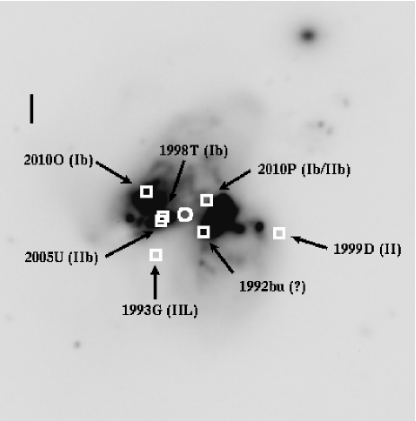
Figure 1: $R$-band image of Arp 299. The eastern structure (to the left of the figure) is known as IC 694, while the western structure is NGC 3690. The positions of all catalogued SNe are marked on the figure using squares, with SN type classification shown in brackets. The scale bar is 2 kpc in length. The image is orientated with east to the left and north up. The circle indicates the system centre as listed in NED.

2.1 The extreme star formation in Arp 299

The numerous starburst regions within Arp 299 were originally studied by Gehrz et al. (1983), who compared its properties in the optical, infrared and radio, identifying a number of regions in the system relating to different starburst components. These naming conventions have continued (and been complemented with further regions for study) in more recent work using spectroscopy and higher resolution (HST) imaging (e.g. Alonso-Herrero et al. 2000; García-Marín et al. 2006; Alonso-Herrero et al. 2009). In later sections of this paper we compare our measurements/analysis to these earlier works, in order to check the validity of our results, and to help understand the system and its SNe.
It is obvious from Fig. 1 that the system is going through a strong interaction and merging event. Arp 299 shows a single tidal tail, indicative of a prograde-retrograde interaction initiated $\sim$700 Myr ago (Neff et al., 2004). While there is likely to be long-term interaction induced SF within this system, Alonso-Herrero et al. (2000) have identified very young starburst regions within Arp 299 that have extremely high SF rates and ages as young as 4 Myr. This latter issue is key to some of the subsequent discussion below when comparing SNe found in Arp 299 to the SF properties of the system. This will be discussed in detail later, however here we make the point that even if these extreme starbursts dominate the current SF in the system, it is highly probable that there are SF episodes of considerably older ages which were induced earlier in the interaction of the two galaxies (note that even prior to the interaction, both of the component galaxies were spiral types, i.e. galaxies containing significant amounts of SF).

2.2 Supernovae discovered within Arp 299

During the past 20 years 7 SNe have been discovered within Arp 299. The positions of these SNe are shown in Fig. 1 along with the type classifications. Searching the Asiago and IAU SN catalogues, the first reported discovery we find is that of SN 1992bu. SN 1992bu was discovered by van Buren et al. (1994) as part of a SN search in starburst galaxies using $K$-band images. This object has no type classification, but for completeness we include the SN in our analysis. The third reported event is SN 1993G (Treffers et al., 1993), discovered as part of the Leuschner Observatory Supernova Search (LOSS, the precursor to the current Lick Observatory Supernova Search). This SN was classified as a type II SN (SNII henceforth) by Filippenko et al. (1993), with a later sub-type classification of SNIIL (Tsvetkov, 1994), where the L signifies the ‘linear’ classification and indicates that in addition to containing hydrogen in its spectrum the SN displayed a linear decline in its light curve (e.g. Barbon et al. 1979). SN 1998T was discovered by the Beijing Astronomical Observatory Supernova Survey (BAOSS) and confirmed by the Lick Supernova survey (Li et al., 1998). It was classified as a SNIb (Li et al., 1998), i.e. hydrogen was lacking in the spectrum but helium was present (see Filippenko 1997, for a review of spectral SN classifications). In the following year SN 1999D was discovered, again by BAOSS (Qiu et al., 1999), and classified as a SNII (Jha et al., 1999) with no further sub-type classification given. SN 2005U was discovered by the Nuclear Supernova Search (Mattila et al., 2005), and originally classified as a SNII by Modjaz et al. (2005), with a later refinement to SNIIb classification (Leonard & Cenko, 2005). SNIIb are thought to be transitional objects being similar to SNII at early times (prominent hydrogen lines), while becoming similar to SNIb at later times (Filippenko et al., 1993). Most recently 2 SNe were discovered at the start of 2010. SN 2010O was found by the Puckett Observatory Supernova Search (Newton et al., 2010), and classified as a SNIb by Mattila et al. (2010). Somewhat surprisingly, the next SN listed on the IAU database, SN 2010P, was also discovered in the interacting system. SN 2010P was found using near-IR images by Mattila & Kankare (2010), and was later classified (Ryder et al., 2010) as SNIb/IIb.

We note here that in the current study we only discuss those SNe that have been discovered using optical and near-IR galaxy images and where definitive classification as true SNe has been possible. While we include one unclassified SN, our conclusions arise from those with classification into various CC types which enables us to infer characteristics of the progenitor population and the underlying SF properties. However, the term ‘supernova factory’ has been coined for this galaxy system through imaging of the system at radio wavelengths. Neff et al. (2004) and Pérez-Torres et al. (2009) (also see Ulvestad 2009) both concluded from radio observations that there are a number of sources which are likely to be recently exploded CC SNe, and that the nucleus of the component IC 694 is thus a ‘supernova factory’, consistent with the presence of very young extreme SF regions as proposed by Alonso-Herrero et al. (2000). Neff et al. (2004) conclude that the detected radio emission of the system implies supernova rates of 0.1-1 yr^-1 (recently Romero-Canizales et al. 2011 also published a lower limit for the SN rate of 0.28yr^-1 from VLA monitoring of the radio emission of the system). Due to the high level of extinction measured in the system (possibly an $A$${}_{\textit{v}}$ of $\sim$ 30 magnitudes in extreme cases; Alonso-Herrero et al. 2000), it is very probable that many of these SNe are missed in optical/near-IR searches. If this extinction preferentially obscures a certain type of event from discovery over others then this may affect the current analysis. We come back to this issue later and discuss it as a possible caveat to our conclusions.

2.3 Core-collapse supernova progenitors

Core-collapse (CC) SNe are generally classified into two broad groups. Those that show signs of hydrogen in their spectra; the type II SNe, and those that do not; the type Ibc (throughout this paper type ‘Ibc’ SNe refers to all those SNe classified as SNIb, SNIc or SNIb/c in the literature). This lack of hydrogen in the latter indicates that their progenitor stars must have lost their envelopes in their pre-SN stellar evolution through some process. Whether this emerges from higher mass/metallicity progenitors producing stonger stellar winds, or from binary interactions is still strongly debated. We will not review all of the literature here (see Smartt 2009 for a recent review of CC SN progenitors), but merely note the work that is most relevant to the current discussion on differences in progenitor characteristics. SNIIP, the most common CC SN type (observed SN rates will be discussed later) are the only class where a number of progenitor stars have been identified on pre-explosion images. Smartt et al. (2009) presented an analysis of direct detections and concluded that SNIIP arise from red-supergiant progenitors between 8.5 and 16.5${\rm\ M}_{\odot}$ (we note the interesting fact that none of the 7 SNe in the current galaxy is classified as IIP). Direct detections of other CC SN types have been few. One of the type II in the current study is a IIL, where the lack of a plateau (found in the IIP), in their light curves is thought to indicate a smaller envelope remaining at the epoch of explosion. One direct detection has been made of a progenitor of a SNIIL, with derived progenitor masses ranging from 11-24${\rm\ M}_{\odot}$ (given the errors from the two studies: Elias-Rosa et al. 2010; Fraser et al. 2010), hence possibly indicating that these SNe arise from slightly higher mass objects than the IIP (however, given a sample of 1, generalising to the whole population is perhaps premature). The IIb class has had two detections of progenitor stars on pre-SN images. Crockett et al. (2008) concluded that SN 2008ax either arose from a single massive star of $\sim$28${\rm\ M}_{\odot}$ or a lower mass binary system, while for the extensively studied SN 1993J, Maund et al. (2004) estimated that the SN arose from an interacting binary with component stars of 14 and 15${\rm\ M}_{\odot}$. Therefore from this small sample the detections suggest that the SNIIb arise from more massive progenitors (whether single or binary star progenitors) than the SNIIP (we also note the likely detection of a massive binary companion star to the SNIIb 2001ig claimed by Ryder et al. 2006). A direct detection of a SNIbc has thus far eluded us (Smartt, 2009), and while upper limits from searches can be put on progenitors, the uncertain nature of current modeling of WR stars (the possible single star progenitors of SNIbc; e.g. Gaskell et al. 1986), means that constraints are less reliable than those for SNIIP.
Other, more indirect constraints can be obtained through studying the nature of the host galaxy emission in close proximity to SN positions. In AJ08 it was shown that SNIbc show a higher degree of asssociation than the SNII population to host galaxy H$\alpha$ emission, implying shorter stellar lifetimes and therefore higher progenitor masses (see also Kelly et al. 2008 for similar results). In the same study the SNIIb also accurately traced the underlying emission (while the SNIIP did not), therefore again implying higher mass progenitors than normal SNII. The SNIIL showed a similar degree of association to the emission as SNIIP implying similar mass progenitors. It therefore seems that progenitor mass is playing a significant role in determining SN type, as suggested by single star models (e.g. Heger et al. 2003; Eldridge & Tout 2004; Georgy et al. 2009).
Progenitor metallicity could also be playing a role in determining SN type. The general consensus seems to be that the SNIbc should arise from higher metallicity progenitors, as this would provide assistance in removing the outer hydrogen envelope, bringing down the progenitor mass at which SNIbc are produced. (We note with reference to the current study that stellar models also generally predict that SNIIb arise from higher metallicity progenitors than SNIIP; e.g. Heger et al. 2003). Observationally this was originally suggested by the centralisation of SNIbc within their host galaxies compared to SNII (e.g. Bartunov et al. 1992; van den Bergh 1997; Tsvetkov et al. 2004; Hakobyan et al. 2009; Anderson & James 2009; AJ09 henceforth). However, the cause of this centralisation has been complicated by work separating host galaxies by signs of interaction/disturbance. In H10 these radial differences were found to be much more prominent in interacting/disturbed galaxies and it was concluded that this was an effect of top-heavy IMFs in the central regions of these galaxies. SNIbc are also found to occur in more luminous (and therefore probably more metal rich) host galaxies (Boissier & Prantzos, 2009), while measurements of the global host galaxy metallicities of SNe (Prieto et al., 2008) found that SNIbc again appeared to arise from higher metallicity hosts. However, in A10, where the gas-phase metallicities of the environments of CC SNe were derived, while a difference was found between the SNIbc and SNII, this difference was found to be small, suggesting that metallicity does not play a significant role in determining SN type (we also note similar studies that concentrated on metallicity differences between SNIb and SNIc environments; Modjaz et al. 2011; Leloudas et al. 2011). Finally, we note that both modeling and observations show that even the highest metallicity environments produce substantial numbers of SNII.
The above discussion shows that while much work has been done in order to further constrain and understand the properties of SN progenitors, disentangling all the different evidence is difficult. The present study attempts to further our understanding by using Arp 299 and its relatively large SN population as a case study, while also using the knowledge implied from the above research to try to further understand the SF properties of the host system.

3 Observations

We obtained our own $R$-band and H$\alpha$ imaging of Arp 299 using the Wide Field Camera (WFC) on the Isaac Newton Telescope (INT). These data and their reduction have been discussed elsewhere (AJ08). Briefly, the $R$-band image was scaled to the H$\alpha$ image and used to continuum subtract the latter, leaving only the emission from HII regions within the system. We also obtained long slit optical spectra of the system, data that was initially presented in A10 (see here for more details of instrument setup, reduction procedures etc). These were obtained with the Intermediate dispersion Spectrograph and Imaging System (ISIS) on the William Herschel Telescope (WHT). The slit positions across the system are shown in Fig. 2. From the literature we use Spitzer 24${\mu}$m imaging, plus near- and far-UV GALEX imaging. These images are shown in Fig. 3 together with our own $R$-band and H$\alpha$ imaging. Here we also show a $K$-band image taken from the literature (Calzetti, 1997). Unlike the other literature images above we do not use the near-IR image in our analysis, but include it in Fig. 3 to show the morphology of this system at different wavelengths.

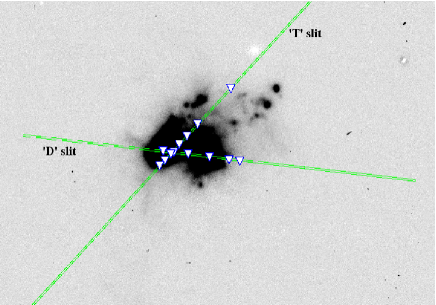
Figure 2: H$\alpha$ continuum subtracted image of the system Arp 299. The two lines show the positions and sizes (1 arcsecond width, 3.7 arcminute length) of the slits that were used to obtain optical spectroscopy of Arp 299. The white triangles indicate the extraction positions for the spectra used to measure any possible metallicity gradients across the system. The image is orientated with north up and east to the left. In the subsequent analysis/discussion the slit positioned at an angle of 131.5 degrees east of north is referred as the ‘T’ slit, while the other is referred to as the ‘D’ slit, as indicated in the figure.

4 Analysis techniques

The main analysis techniques used throughout this work are those detailed in AJ08, AJ09, and A10. Here we briefly summarise those statistical methods but we refer the reader to those references for a full discussion of the methods and associated errors. We note that for three SNe these statistics (at least with respect to the H$\alpha$ and $R$-band emission of their host galaxies) have already been presented in previous papers; SN 1993G, SN 1998T and SN 1999D, but for the three most recent SNe (SN 2005U, SN 2010O and SN 2010P, plus the unclassified SN 1992bu) we present new analysis (note that SN 2005U had been discovered at the time of publication of those previous works, however in the catalogues its host galaxy is listed as Arp 299 and not NGC 3690 as were all others, and therefore the SN was missed).
In James & Anderson (2006) we introduced a statistic which normalises the count found within one pixel of a galaxy of some light emission (in that case H$\alpha$), to the overall counts of the galaxy (around the same time a very similar technique was presented by Fruchter et al. 2006, although these authors used the continuum blue light as a tracer of SF). This statistic then gives a value between 0 and 1 for each pixel on the image, where 0 indicates a region of zero emission or sky, while a value of 1 indicates the centre of the brightest region of the galaxy. One can then use this statistic to study the overall association of a certain type of object to e.g. the underlying H$\alpha$ emission of their host galaxies, where a higher mean pixel value indicates a higher degree of association of that object type to the emission. We calculate pixel values (dubbed NCR values in AJ08) for all SNe with respect the H$\alpha$, 24${\mu}$m, near-UV and far-UV emission and compare these to the overall distributions previously found in AJ08.
One can also investigate SN progenitor and SF properties by investigating the radial distribution of different SNe within host galaxies. In AJ09 we presented results on the radial positions of different SN types where we calculated the amount of host galaxy light found within an ellipse or circle just including the SN position, normalised to the total galaxy. We measure these same radial values, referred to as Fr values, for all SNe, with respect to the $R$-band, H$\alpha$, 24${\mu}$m, near-UV and far-UV emission found within the system. However, one can easily see when looking at Fig. 1 that this type of analysis is complicated in a galaxy system of this nature due to the irregular morphologies involved and problems defining a galaxy centre (the central point listed in NED and used in AJ09 is shown by the circle in Fig. 1). We discuss these issues below, while also deriving alternative radial measurements with respect to the centres of the peak of the stellar mass.
Finally we derive metallicities for the local environments of each SN, from the ratio of strong emission lines found within the host (or nearby) HII regions and assume these as progenitor metallicities, using long slit optical spectra. To estimate metallicities from our spectra we follow the procedures outlined in A10 using the Pettini & Pagel (2004) (PP04 henceforth) ‘empirical’ line diagnostics. These methods have the advantage of being relatively insensitive to extinction, due to the close proximity (in wavelength) of the emission lines used to derive metallicities. Using the same long slit observations we also extract numerous spectra along each slit (shown in Fig. 2) to search for any possible metallicity gradients across the system.
In Fig. 3 we show example spectra extracted close to the position of the SN 2010P, marking the emission lines that we use in our metallicity derivations.

Figure 3: Example spectra showing the red (top) and blue (bottom) arms of the ISIS spectra extracted at the closest position along the slit to the position of the SN 2010P. The positions of the emission lines used for the metallicity derivations are shown.

5 Results

SN	Type	NCR${}_{\textit{H$\alpha${}}}$	NCR${}_{\textit{Spitzer}}$	NCR${}_{\textit{nUV}}$	NCR${}_{\textit{fUV}}$	Fr${}_{\textit{R}}$	Fr${}_{\textit{H$\alpha${}}}$	Fr${}_{\textit{Spitzer}}$	Fr${}_{\textit{nUV}}$	Fr${}_{\textit{fUV}}$
1992bu	?	0.321	0.922	0.649	0.323	0.056	0.055	0.263	0.165	0.148
1993G	IIL	0.064	0.193	0.194	0.098	0.464	0.744	0.761	0.534	0.514
1998T	Ib	0.578	0.829	0.870	0.723	0.056	0.106	0.164	0.116	0.113
1999D	II	0.054	0.122	0.263	0.407	0.560	0.849	0.990	0.899	0.895
2005U	IIb	0.672	0.621	0.870	0.723	0.095	0.106	0.195	0.116	0.113
2010O	Ib	0.421	0.559	0.508	0.285	0.414	0.655	0.682	0.483	0.459
2010P	Ib/IIb	0.406	0.662	0.563	0.414	0.095	0.106	0.195	0.138	0.129

Table 1: NCR pixel values and fractional radial values for all SNe within Arp 299. In the first column the SN name is given followed by the type classification. Then in columns 3 through 6 the NCR pixel values are listed for each SN with respect to the H$\alpha$, 24${\mu}$m, near-UV and far-UV emission respectively. Then in columns 7 through 11 the fractional radial values are listed for each SN with respect to the $R$-band, H$\alpha$, 24${\mu}$m, near-UV and far-UV emission respectively.

5.1 Pixel statistics

The pixel statistics of each SN calculated from the different wavelength observations, together with the radial statistics are listed in Table 1. The mean NCR H$\alpha$ pixel value for the two non-IIb SNII is 0.059, i.e. both of these SNe fall on regions with little H$\alpha$ emission. For the SNIb (including the value for SN 2010P at half weighting given the intermediate type classification of Ib/IIb), the mean is 0.481 and these SNe all fall on bright HII regions within the system. The mean value for the SNIIb (again taking half weighting from SN 2010P) is 0.583. Finally the overall ‘stripped envelope’ population has an H$\alpha$ NCR mean value of 0.519. Hence both the SNIb and SNIIb show a higher degree of association to the line emission than the other SNII. This is consistent with the results from AJ08. We also note that the slightly higher degree of association of the SNIIb to the emission than the SNIb is consistent with that seen from the larger galaxy samples studied previously.
In a merging system such as Arp 299 there will be a high level of extinction due to dust. Therefore H$\alpha$ emission may not provide the most reliable indicator of the distribution of SF. Emission in the mid-IR should be a sensitive tracer of such a dust-embedded SF component. We therefore also calculate the NCR values for all SNe with respect to mid-IR emission at 24${\mu}$m as imaged by Spitzer. The mean NCR 24${\mu}$m value for the two non-IIb SNII is 0.158, 0.688 for the SNIb, and 0.635 for the SNIIb, with a value of 0.668 for the overall ‘stripped envelope’ population. Hence almost identical trends are seen in the mid-IR as shown by H$\alpha$; the SNIb and SNIIb show a much higher degree of association to the recent SF hence implying shorter pre-SN lifetimes and higher progenitor masses.
The pixel values derived for the near- and far-UV emission from GALEX images again show similar trends to the above, with NCR values for the individual SNe being slightly higher than with respect to the H$\alpha$ emission. UV emission traces recent SF down to lower stellar masses and therefore this is to be expected and shows that while the ‘normal’ SNII do not fall on the brightest HII regions, they are still found to occur on regions of recent SF, only those traced by lower mass stars than H$\alpha$ line emission.
Almost exclusively in all tracers of SF the ‘stripped envelope’ SNe fall on higher pixel count regions of Arp 299 than the ‘normal’ SNII (the only anomaly is the NCR far-UV value for SN 1999D in comparison to that of SN 2010P). Using this fact that all the 4 SNe Ib/IIb have higher NCR values than the other SNe we calculate a $\sim$7% probability of this occurring by chance, if one assumes that in the true underlying distribution all SNe are equally distributed on SF regions.

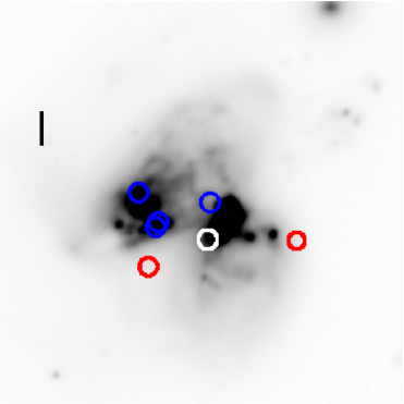
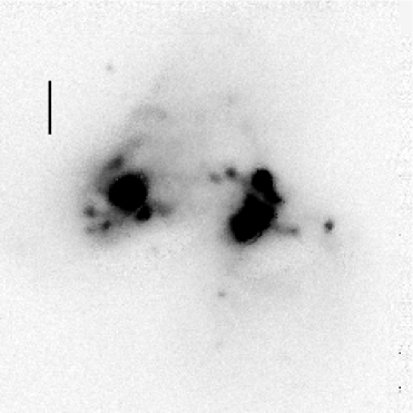
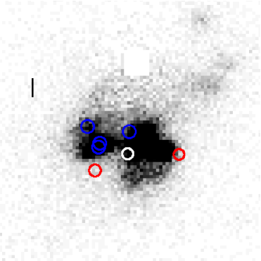
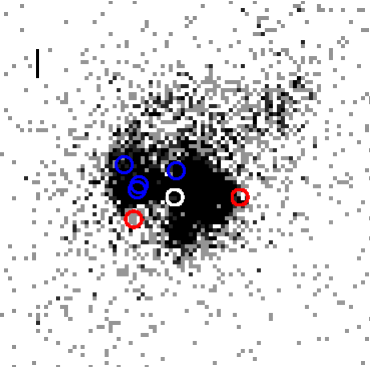
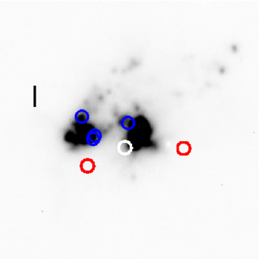
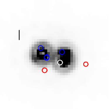
Figure 4: Images of Arp 299 at different wavelengths. Top left shows an $R$-band image with a $K$-band image shown top right (the $K$-band image does not have the SNe positions marked as the image is not astrometrically calibrated). In the middle panel the GALEX near-UV (left) and far-UV (right) images are shown. In the bottom panel we show the H$\alpha$ image on the left and Spitzer image on the right. On each image a scale bar shows a distance of 2 kpc, and the SNe positions are indicated by the coloured circles: the ‘stripped envelope’ SNe (Ib and IIb) are shown in blue circles, while the ‘normal’ SNII are shown in red. The unclassified SN 1992bu is shown in white.

5.2 Radial positions of SNe

We derive Fr values here with respect to Arp 299 central coordinates given in NED. This puts the centre midway between the two galaxy components (shown in Fig. 1), which may be ambiguous, given that there are definitely (at least) two peaks in the emission of the merging system. In AJ09 when dealing with interacting or irregular galaxies either the two galaxies were treated separately or the central point of the $R$-band emission was used. Arp 299 is probably the only galaxy within that earlier sample where uncertainties in the central location might significantly affect the conclusions drawn. We present the Fr statistics for all SNe in the sample, and below proceed with additional analysis to test the reliability of these results. The mean Fr${}_{\textit{R}}$ for the 2 SNII is 0.512. For the SNIb the mean value is 0.207 while for the SNIIb the mean Fr${}_{\textit{R}}$ value is 0.095, with an overall mean ‘stripped envelope’ value of 0.165. Hence both the SNIb and SNIIb are more centrally concentrated with respect to the $R$-band emission than the other SNII. In fact every individual SNIb and SNIIb is found closer to the central point of the system than the SNe 1993G and 1999D.
Again, very similar radial trends are found with respect to all other emission tracers used. This consistency of results across wavelength (here for the radial analysis and above for the pixel statistics analysis) increases the robustness of the results presented.

5.2.1 With respect to separate galaxy components

The merging nature of the system Arp 299 makes it almost impossible to separate the two components to allow for an unbiased study of the radial positions with respect to the emission of the system. One way to investigate the radial positions further is to derive projected distances of each SN to the peaks of the stellar mass of each system, as determined from the peak of the $K$-band emission from 2MASS (Skrutskie et al., 2006) images. Here we determine distances for each SN from component $A$ (IC 694) and component B1 (brightest peak of NGC 3690), following the naming conventions used in the literature (e.g. Gehrz et al. 1983; Alonso-Herrero et al. 2000). These distances are listed in Table 2.
Associating each SN with the galaxy component in closest proximity we can again compare the values for the different SN types. For the two ‘normal’ SNII we find a mean distance of 3.82 kpc from their host nuclei. For the SNIb this value is 1.20 kpc while for the SNIIb the mean is 1.33 kpc. The overall ‘stripped envelope’ mean distance is 1.25 kpc. Hence while there are some small differences between the radial values here and those above (e.g. SN 2010O is considerably more central when this projected distance analysis is achieved), the overall trends are again the same; the SNII are found further from the nuclei of the components of Arp 299 than both the SNIIb and the SNIb.
We also re-do the Fr analysis discussed above, centering the radial apertures used to measure galaxy emission fluxes on the central positions of NGC 3690 (B1) and IC 694 ($A$). It is difficult to assess where one galaxies’ emission stops and the other starts due to the interaction of this system. Therefore here we include all of the emission of the system in the analysis. While this will not give true Fr values for each galaxy component, one can still look at the relative Fr values between the different SNe, and this is what we wish to test; do we still see the trends from above that all the ‘stripped envelope’ events are more centrally concentrated than the other ‘normal’ SNII? The results of this analysis are shown in Table 3. Again we see almost identical trends: almost exclusivley the Fr values are lower for all ‘stripped envelope’ events than for the other two SNe, and this is seen across all wavelengths analysed.
As for the pixel stats above, we calculate the probability of this trend occurring by chance, and the value is the same: $\sim$7%, that 4 events from 6 are closer to the centres of the system assuming that the underlying distribution is uniform across the whole galaxy.

The centralisation of SNIb and SNIIb over the other SNII is more difficult to interpret than the pixel statistics above. If these SNe were occurring in a normal spiral galaxy then one would probably infer that this centralisation were due to a metallicity effect. However, in a merging/interacting system such as Arp 299 any metallicity gradient is likely to be smoothed out by the inflow of gas; indeed we show this to be the case using our metallicity derivations below. Other explanations include these central regions being too young to have produced many lower mass, longer stellar lifetime SNII to date, or that in these central regions the IMF is biased towards higher mass stars and hence is producing more SNIb and SNIIb over normal SNII. These final two points provide the main discussion points from this work and we return to them in detail in latter sections.

SN	Type	kpc ($A$)	kpc (B1)
1992bu	?	4.11	1.13
1993G	IIL	3.37	4.69
1998T	Ib	0.98	3.77
1999D	II	8.71	4.27
2005U	IIb	1.10	3.85
2010O	Ib	1.13	5.46
2010P	Ib/IIb	3.74	1.79

Table 2: Distances (in kpc) of each SN from the nuclei of both NGC 3690 and IC 694.

SN	Type	Fr${}_{\textit{R}}$($A$)	Fr${}_{\textit{H$\alpha${}}}$($A$)	Fr${}_{\textit{Spitzer}}$($A$)	Fr${}_{\textit{nUV}}$($A$)	Fr${}_{\textit{fUV}}$($A$)	Fr${}_{\textit{R}}$(B1)	Fr${}_{\textit{H$\alpha${}}}$(B1)	Fr${}_{\textit{Spitzer}}$(B1)	Fr${}_{\textit{nUV}}$(B1)	Fr${}_{\textit{fUV}}$(B1)
1992bu	?	0.353	0.359	0.413	0.344	0.281	0.131	0.117	0.046	0.120	0.096
1993G	IIL	0.277	0.320	0.381	0.260	0.235	0.511	0.426	0.469	0.705	0.734
1998T	Ib	0.068	0.117	0.050	0.046	0.037	0.384	0.338	0.401	0.574	0.597
1999D	II	0.841	0.942	0.763	0.919	0.920	0.511	0.426	0.490	0.692	0.724
2005U	IIb	0.068	0.117	0.070	0.059	0.050	0.423	0.359	0.401	0.613	0.645
2010O	Ib	0.068	0.117	0.121	0.059	0.050	0.596	0.623	0.604	0.773	0.793
2010P	Ib/IIb	0.311	0.338	0.352	0.308	0.264	0.252	0.267	0.285	0.299	0.289

Table 3: Fractional radial values (Fr) for all SNe with respect to the centres of both IC 694 ($A$) and NGC 3690 (B1). Columns 3 through 7 list the Fr values with respect to $A$ and analysed with respect to the $R$-band, H$\alpha$, Spitzer, near and far-UV emission respectively. While columns 8 through 12 list the same values but with respect to B1.

5.3 Environment metallicities of SNe

In Table 4 we present the environment metallicities for all SNe discovered in Arp 299, together with their associated errors. These metallicities are logarithmic oxygen abundances, relative to hydrogen ([O/H]), which are derived using the PP04 O3N2 and N2 emission line diagnostics. These are derived from spectra extracted at the closest position along the slit to the catalogued SN coordinates. This means that in some cases the environment metallicity is derived at a significant distance away from the actual SN position. These distances are listed in column 6 of Table 4.
One may therefore question whether these derived metallicities are truly representative of those of the actual SN positions, or even the ‘true’ environment where the progenitor was formed (even given the short stellar lifetimes of progenitor stars, it is still possible, or even likely that stars will explode at considerable distances from where they were formed; see James & Anderson 2006 and A10 for additional discussion). The environment metallicities of SNe 1998T and 2005U were both derived very close to the catalogued positions, and hence we are confident that these should be representative of the abundances of the actual progenitors. For all other environment abundances were derived at $\sim$1 kpc or more from the SN coordinates. Hence these values should be taken as a ‘best guess’ of the true progenitor metallicities. However, as many SNe occur away from bright HII regions it is almost impossible to derive ‘true’ emission line metallicities (this is the case for SNe 1993G and 1999D in the present study). Therefore we note this caveat to the values we present in Table 4, but continue with the analysis, assuming these metallicities represent the abundances near to the regions where these SNe exploded.
Looking at the environment metallicities presented in Table 4 we see that the inferred progenitor metallicities for all SNe discovered in Arp 299 are very similar, with the largest difference between any two being 0.08 dex. For the two SNII we find a mean oxygen abundance, using the 03N2 diagnostic of the PP04 scale of 8.55. For the SNIb this metallicity is 8.58 while for the SNIIb the mean is 8.54. For the overall ‘stripped envelope’ population we derive a mean of 8.56. Hence all the environment metallicities for the different types are identical within the errors.
We also compare our inferred progenitor metallicities with those derived for larger samples in the literature. In A10 CC SN progenitor metallicities for 46 SNII (dominated by SNIIP), 10 SNIb and 14 SNIc were published. The mean value for the SNII was 8.58, while for the SNIb the mean was 8.62. Hence within the errors the values derived for the smaller samples here are consistent with the mean values from A10; i.e. the inferred progenitor metallicities for SNe in Arp 299 are neither metal rich nor metal poor when compared to the overall populations studied previously. However, SNIb, SNIIb and SNIc environment metallicities have also recently been published by Modjaz et al. (2011) and Leloudas et al. (2011). For the SNIb samples (Modjaz et al. 2011 group the SNIIb in this sample as well), these authors find mean metallicities (on the PP04 scale) of 8.41 (Modjaz et al., 2011) and 8.52 (Leloudas et al., 2011). Hence with respect to these studies, the SNIb and SNIIb metallicities we derive here may be considered slightly metal rich. However, the reasons for these different metallicity estimates in different studies is not yet clear, and we note that while the above comparisons are interesting they do not affect the overall conclusions we present in this paper. To resolve these issues it is likely that we will have to wait for larger samples of metallicities to be published where all SNe are taken from ‘blind’ SN searches.
Finally in this section we compare the ratio of SN types found here with those found in the same metallicity range in A10. The mean of the 6 classified SNe in Arp 299 is 8.56 with a standard deviation of 0.05 dex. Taking all SNe that fall in this metallicity range (8.50 to 8.61) from A10 we find a ratio of ‘normal’ SNII to ‘stripped envelope’ SNe of 2.6. The A10 sample was a very heterogeneous group of SNe, but this ratio agrees well with that seen in nearby galaxies, at all metallicity ranges (Li et al. 2011). However, the ratio of events we find in Arp 299 is 0.5. Hence, this is further confirmation that differences in metallicity does not appear a viable explanation for the types and distribution of SNe found in this system.

The central parts of Arp 299 suffer from high levels of extinction (e.g. Alonso-Herrero et al. 2000). Therefore one may worry that the metallicities derived for circumnuclear regions (where the majority of the SNe are found) may be significantly in error. As discussed in A10, the extracted spectra of Arp 299 were not corrected for host galaxy extinction as the spectra were not taken at the parallactic angle. However, as we use the PP04 diagnostics using emission lines close in wavelength, this effect should only be marginal. We check this assumpition using the spectrum of the environment of SN 2010P (shown in Fig. 3). Mattila et al. (2010) and Ryder et al. (2010) reported an A_v of $\sim$5 for SN 2010P, estimated from SN near-IR photometry and a deep optical spectrum. Therefore we de-redden our SN enviroment spectrum by this amount (note that the spectrum was not taken at the same position as SN 2010P, and therefore this comparison will be in error somewhat, however this is solely an example of the effects of extinction). We then re-measure line fluxes and re-estimate our environment metallicity values for SN 2010P. For the PP04 N2 diagnostic we measure a new abundance of 8.69${}^{+0.19}_{-0.19}$, 0.01 dex lower than the value reported in Table 4. While for the O3N2 diagnostic we measure a new abundance of 8.61${}^{+0.14}_{-0.14}$, 0.02 dex higher than that reported in Table 4. Hence, we conclude that even if there are large levels of environment extinction in Arp 299, which we have not corrected for, the effect of these will be negligible on our derived metallicities and hence the conclusions of this work.

5.3.1 Comparison to literature values

Arp 299 has been extensively observed and studied in the literature. One such study by García-Marín et al. (2006, G06 henceforth) published emission line ratios for various regions across the system, using IFU observations. Hence, as a sanity check we compare our derived environment metallicities with those calculated from the emission line ratios published in G06. We determine the nearest emission region in G06 to our SN environment regions listed in Table 4. We can then compare our metallicities with those derived from the flux ratios in G06. The results from this comparison are shown in Table 5 and they illustrate that in general our derived environment metallicities agree extremely well with those measured in nearby regions taken from G06, even though all of the regions compared are at least 0.2 kpc in separation. There are two cases where considerable metallicity differences are found. For SN 1992bu we find a metallicity difference of 0.14 dex. However, here we associate the SN environment with the nucleus of NGC 3690, region B1, where one may find much more extreme conditions than outside this region, where our metallicity value is determined (0.8 kpc away). Indeed, in regions B11 and B16 which are outside the main nucleus of NGC 3690 and only slightly further away from our environment position than B1, the metallicities one derives from the line ratios in G06 are completely consistent with our values. Therefore we are not worried by this discrepancy. A difference (0.08 dex) is also found between the environment of SN 2010P and the value taken from the literature. However, again if we compare our value with other nearby regions in G06 such as K6 or K7 (which are separated to a similar degree to the separation between our environment and that taken from the literature), we find a much better agreement.
In Table 5 we have listed the distances between the coordinates of the extracted spectra we use for metallicity derivations, and the closest regions in G06 used for the above comparison. As many of our metallicities are derived from regions at significant distances from the catalogued SN positions one may wonder whether some of the abundances derived from the emission line fluxes in G06 may actually better represent those of the SNe currently studied. However, calculating the projected distances between the G06 regions used above (and indeed other regions in G06 that may be closer to the SNe coordinates), we find that all but one (SN 2010P, and here the difference is only 0.02 kpc) of our extracted spectra are closer to the SN position than any regions studied in G06.
Finally we note that even if we were to take the above literature metallicities in place of our own values, the implications for the current study would not change; there are no significant differences in the environment (and therefore progenitor) metallicities between the different types of SNe found to occur in this interacting system.

SN	Type	N2	O3N2	Extraction coordinates	Distance from SN position (kpc)
1992bu	?	8.76${}^{+0.19}_{-0.19}$	8.60${}^{+0.14}_{-0.14}$	11 28 31.33 +58 33 42.9	1.04
1993G	IIL	8.56${}^{+0.19}_{-0.19}$	8.51${}^{+0.14}_{-0.14}$	11 28 33.87 +58 33 37.4	1.61
1998T	Ib	8.60${}^{+0.18}_{-0.19}$	8.53${}^{+0.14}_{-0.14}$	11 28 33.16 +58 33 43.7	SN
1999D	II	8.75${}^{+0.19}_{-0.19}$	8.59${}^{+0.14}_{-0.14}$	11 28 28.77 +58 33 40.5	0.73
2005U	IIb	8.60${}^{+0.18}_{-0.19}$	8.52${}^{+0.14}_{-0.14}$	11 28 33.26 +58 33 42.8	0.10
2010O	Ib	8.72${}^{+0.19}_{-0.19}$	8.63${}^{+0.14}_{-0.14}$	11 28 33.95 +58 33 45.2	1.36
2010P	Ib/IIb	8.70${}^{+0.19}_{-0.19}$	8.59${}^{+0.14}_{-0.14}$	11 28 31.81 +58 33 53.1	1.07

Table 4: Metallicity derivations for the closest HII region to the positions of each SN. In the first column the SN name is listed, followed by the type classification. In columns 3 and 4 the [O/H] abundances are given for each SN, derived from the PP04 N2 and O3N2 diagnostics, together with their associated errors; a combination of the flux calibration error, the statistical error in the continuum at the position of the line measurements, and the calibration error taken from PP04. In all cases this last calibration error dominates the overall metallicity error. Then the coordinates are given for the extraction position (epoch J2000) of the spectrum used to derive the environment metallicities. Finally the distance from the SN explosion position to that of the extracted spectrum is listed (‘SN’ indicates that the extraction was achieved at the SN position).

SN	G06 region	Metallicity difference (dex)	Distance (kpc)
1992bu	B1	-0.14	0.8
1993G	G	0.00	1.0
1998T	A6	0.03	0.3
1999D	D3	0.01	2.1
2005U	A6	0.03	0.4
2010O	A1	0.04	0.2
2010P	K5	-0.08	0.5

Table 5: Metallicity differences between the SN environments (column 1) and regions taken from G06 (column 2). The metallicity differences are listed in column 3 where a positive value indicates that the literature value is higher than that derived in the current work, followed by the distance between the two regions in column 4. Note that these regions are not necessarily the closest to the SN position, but are the closest to the region used to infer the SN environment metallicities.

Extraction ID	N2	O3N2	Coordinates
1D	8.71${}^{+0.19}_{-0.19}$	8.62${}^{+0.14}_{-0.14}$	11 28 33.73 +58 33 45.0
2D	8.66${}^{+0.19}_{-0.19}$	8.59${}^{+0.14}_{-0.14}$	11 28 32.98 +58 33 44.3
3D	8.69${}^{+0.19}_{-0.19}$	8.61${}^{+0.14}_{-0.14}$	11 28 31.95 +58 33 43.4
4D	8.79${}^{+0.19}_{-0.19}$	8.58${}^{+0.14}_{-0.14}$	11 28 30.44 +58 33 42.1
5D	8.75${}^{+0.19}_{-0.19}$	8.56${}^{+0.14}_{-0.14}$	11 28 29.83 +58 33 41.5
6D	8.75${}^{+0.19}_{-0.19}$	8.60${}^{+0.14}_{-0.14}$	11 28 29.02 +58 33 40.8
1T	8.69${}^{+0.19}_{-0.19}$	8.55${}^{+0.14}_{-0.14}$	11 28 33.98 +58 33 36.5
2T	8.65${}^{+0.19}_{-0.19}$	8.54${}^{+0.14}_{-0.14}$	11 28 33.61 +58 33 39.7
3T	8.59${}^{+0.18}_{-0.19}$	8.55${}^{+0.14}_{-0.14}$	11 28 33.20 +58 33 43.4
4T	8.70${}^{+0.19}_{-0.19}$	8.61${}^{+0.14}_{-0.14}$	11 28 32.61 +58 33 48.6
5T	8.69${}^{+0.19}_{-0.19}$	8.59${}^{+0.14}_{-0.14}$	11 28 32.04 +58 33 53.6
6T	8.78${}^{+0.19}_{-0.19}$	8.56${}^{+0.14}_{-0.14}$	11 28 31.30 +58 34 00.2
7T	8.69${}^{+0.19}_{-0.19}$	8.59${}^{+0.14}_{-0.14}$	11 28 28.99 +58 34 20.6

Table 6: Metallicity values for the various slit positions indicated in Fig. 2. The number before the letter ‘D’ or ‘T’ indicates the extraction position along the slit with the number one extraction being that furthest to the left (east) of the galaxy image in Fig. 2. For each slit position the environment abundances are listed together with their associated errors, followed by the coordinates of the extraction position (epoch J2000).

5.4 Metallicity gradients in Arp 299

Using the slit positions as shown in Fig. 2 we can also investigate whether there are any metallicity gradients across the system. Spectra were extracted at the positions shown in Fig. 2 and metallicities were derived in the same way as above for the environment HII regions. These metallicities are listed in Table 6 where the numbers followed by ‘D’ refer to the SN 1999D slit position (centred close to the position of SN 1999D with a position angle of 83.4 degrees east of north) and those referred to as numbers followed by ‘T’ refer to the SN 1998T slit position (centred close to the position of SN 1998T with a position angle of 131.5 east of north).
One can see in Table 6 that we find no gradients across the system, and indeed very little variation in metallicity from environment to environment. This is completely consistent with the above SN environment metallicities and reinforces the finding that nearly all environments within the interacting system Arp 299 have very similar gas-phase metallicities. This is also consistent with recent work (Kewley et al., 2010) that has found that metallicity gradients within interacting galaxy pairs are much shallower or even non-existent when compared to normal isolated spirals.

5.5 Relative rates of SNe in Arp 299

One of the motivations for this case study was the suggestion that the SNe types that have been discovered in the system are dominated by the ‘stripped envelope’ CC SNe (i.e. the Ib, Ic or IIb). In this section we analyse this hypothesis. 6 SNe with classifications have been found in the system; one SNII (no further classification), one SNIIL, one SNIIb, two SNIb and an event classed as only Ib/IIb. Above we have considered three groups; the ‘normal’ type II (in which we include the SNIIL), the IIb and the Ib, while also considering the ‘stripped envelope’ SNe as an overall group. Calculating a ratio of ‘normal’ SNII to ‘stripped envelope’ events we find a value of 0.5 in Arp 299. We can then compare this value to nearby SN rate measurements. The most recent rates were measured and published by the LOSS group (Li et al., 2011). From their measured rates we find a ratio of $\sim$2; a factor of 4 higher than that found in Arp 299.
To calculate the probability of finding the observed SN type distribution in Arp 299 we use a Monte Carlo analysis to draw 6 SNe randomly from the overall nearby CC SN rates published by Li et al. (as percentages of the CC SN population we derive: 52% SNIIP, 7% IIL, 9% IIb, 7% IIn, 7% Ib and 18% Ic). We can then derive the probability of detecting a ratio of ‘normal’ type II SNe to ‘stripped envelope’ events equal to or less than the value of 0.5 we find in the current analysis. Note, here we include the SNIc in the ‘stripped envelope’ group for the probability analysis, even though there are no SNe of this type detected in the galaxy; this is to be consistent with the separation of SNe throughout the above analysis into those the in ‘stripped envelope’ class and those that are not (we also note there is some ambiguity in the clasification of some SNe between the Ib and Ic subtypes; Leloudas et al. 2011). We derive a probability of $\sim$10% that one would find a ratio equal to or less than that found here. Hence there is marginal statistical evidence that the number of ‘stripped envelope’ events is higher in this merging system than that found in nearby galaxies. (If we were not to include the SNIc in the probability analysis, and derive the likelihood of finding a ratio of Ib and IIb events to all others of less than or equal to 0.5, this probability drops to 0.8%). However, we note that SNIIL (SN 1993G) are relatively rare events and one may consider these ‘stripped envelope’ events when compared to SNIIP (i.e. SNIIL have smaller hydrogen envelopes at the time of explosion). Hence if we were to include this in the probability calculation, we find only a 5% chance that if we were to draw a sample of 6 SNe randomly from those found in nearby galaxies we would find a ratio of 1:5 of ‘normal’ SNII to other CC types. Finally we note that even this probability may be an overestimation, given the undistinct sub-type classification of SN 1999D.
Within Arp 299 there is one unclassified SN; 1992bu. To estimate the error on the above chance probability, we can re-run our Monte Carlo simluation assuming that SN 1992bu is either a ‘stripped envelope’ or ‘normal’ event. We find a probability of $\sim$5% if we include the SN in the former, and a probability of $\sim$19% if we were to include the SN in the latter (that we observe the detected SN type distribution by chance assuming underlying SN rates found in the local Universe). In section 6.4 we argue that given the environment of SN 1992bu (high degree of association to SF tracers, found to occur centrally), it is more probable that the SN was of the ‘stripped envelope’ type. Hence if we take this to be true, the claim of a relatively higher rate of ‘stripped envelope’ events to ‘normal’ SNII in Arp 299 would be strengthened.

6 Discussion

In the previous sections we have presented various analyses investigating the relative numbers of different SN types, together with the positions at which they are found within their host galaxy system. Overall we find that the ratio of ‘stripped envelope’ CC SNe to ‘normal’ type II events is higher than that found in samples of nearby galaxies, and that the former are much more centrally concentrated within the system than the latter. In the following sections we discuss the possible implications of these findings, both on SN progenitor properties and the nature of the SF found within this system.

6.1 The environments of SNe within Arp 299

The ‘stripped envelope’ SNe are all found to occur more centrally with respect to the stellar populations traced by different wavebands, and also with respect to the peaks in the stellar mass distribution of the two galaxy components than the other SNII. Usually such centralisation would be attributed to a metallicity affect. However, as we show above, no metallicity gradients exist within this system and abundance derivations close to the sites of each SN position show no preference for the ‘stripped envelope’ events to occur in higher metallicity environments. These SNe are also found to occur within bright HII regions within the system, while the other SNII are found further from such high mass star tracers. This implies that the latter have arisen from lower mass progenitors, consistent with previous results looking at large samples of CC SNe in nearby galaxies (AJ08).

6.2 Starburst age effect

One possibility that may explain the relatively high occurrence of ‘stripped envelope’ events is that the majority of the SF within the system is too young for the ‘true’ SN rates (assuming a non-varying IMF) to be observed. This would be consistent with the very young ages of the most recent SF episodes within system found by G06. These authors generally find ages for the HII regions found within Arp 299 between 3-7 Myr. If SNIbc arise from single star progenitors then they are likely to arise from stars more massive than 25${\rm\ M}_{\odot}$ (e.g. Heger et al. 2003; Meynet & Maeder 2005). From the models of Meynet & Maeder (2005) this corresponds to a pre-SN progenitor age (summing the hydrogen and helium burning timescales) of $\sim$8 Myr. Hence this is reasonably consistent with the interpretation that the dominant current SF within the merging event is on timescales where only stars of masses consistent with those for SNIbc and indeed the overall ‘stripped envelope’ class have had sufficient time to explode as SNe (it is indeed possible that we are observing the system at such a specific time when all of the most massive stars have already exploded as SNIc and hence we do not observe any of these SNe, but SF within the system is not old enough to be dominated by SNIIP explosions and hence we find an overabundance of SNIb and SNIIb).
If this is indeed the case then the relative numbers of SNe within Arp 299 provides independent (from that presented in AJ08) observational evidence that SNe of type Ib and IIb arise from shorter lived and hence more massive progenitors than other ‘normal’ type II events. This line of reasoning also gives further evidence for the progenitor mass sequence suggested in AJ08. Here, the reason we do not observe any SNIc (as outlined above) is because the most massive stars have already exploded as SNIc. The lack of SNIc and the overabundance of SNIb/IIb then suggests a progenitor mass sequence from SNII arising from the lowest mass stars, through the SNIb and SNIIb, and finally the SNIc arising from highest mass progenitors. (We make an important point here: this does not necessarily favour single star progenitors for these events over binary progenitor scenarios. One can easily envisage a scenario where some, possibly the majority of these events arise from binaries, but the components of those binaries are indeed more massive and have shorter lifetimes than those that explode as SNIIP or SNIIL events.) This is also consistent with the work of Nelemans et al. (2010), who tentatively concluded that the progenitor of the SN 2010O (type Ib) was a massive Wolf-Rayet star from analysis of Chandra pre-explosion images.
There are however a number of caveats to this interpretation. Firstly, the ages published for SF regions studied by G06 represent the ages of the most recent extreme SF. The above interpretation would require either that before these episodes there was very little SF taking place, or that the SF rate over the last few Myr is much higher than that previously meaning that SNe produced from these recent events will dominate over those produced by older but longer duration SF episodes. However, the interaction/merging of the two components of Arp 299 has probably been active for at least a few 100 Myr and therefore it is difficult to see why the SF from the last few Myr should be so dominant. Indeed, we do find 2 SNe classified as SNII which we presume to have lower mass progenitors, and therefore there is ample evidence for significant SF over timescales longer than that found in previous studies, and that required to produce the high number of ‘stripped envelope’ SNe seen in this study. It is also not clear how this interpretation would explain the centralisation of the ‘stripped envelope’ SNe over the other 2 SNII. One could envisage a scenario whereby the majority of the SF is happening towards the central parts of the system, then the longer lived progenitor (those of the SNII) have time to drift away from the central regions before exploding. However, this would require that the SF within these central regions has been active and continuous for timescales longer than those quoted above, and indeed this would then not explain why there are so many of the ‘stripped envelope’ SNe with respect to the others.
In conclusion to this section, it is very possible that the age of the recent extreme SF currently occurring in Arp 299 could explain some of the results we present in this work. However, for this to be true a number of (in our opinion) unlikely coincidences would have to be at play. Therefore we argue that there are probably other factors affecting the observed distribution of SNe in Arp 299 which we now discuss.

6.3 Comments on IMF interpretation

In H10, we demonstrated that SNIbc show a striking degree of central concentration in disturbed host galaxies, and that the central regions of these systems produce a remarkably small fraction of SNII. Disturbed galaxies are known to experience nuclear starbursts, with Arp 299 being a classic example, and several studies (see H10 for further details) have inferred that these starbursts are likely to exhibit a modified stellar initial mass function (IMF), biased to produce relatively more high mass stars than a ‘standard’ IMF (e.g. Salpeter 1955). Such a modified IMF gives a natural explanation for an enhanced fraction of ‘stripped envelope’ SNe, if the latter result from higher-mass progenitors than SNII, as was found by AJ08. Indeed, Klessen et al. (2007) suggest a specific mechanism for modifying the IMF in starbursts which suppresses or completely prevents the formation of all stars below a given mass limit, which could explain the deficiency of SNII found in disturbed galaxy centres. The predictions of this model for CC SN fractions generally will be explored in a later paper (James et al. in preparation), but it is interesting to note that the Klessen model requires a high-temperature intergalactic medium, with a consequent raising of the Jeans mass, a prediction that seems to be strongly confirmed in the case of Arp 299. The IRAS 60$\mu$m/100$\mu$m flux ratio for Arp 299/NGC 3690 is 1.01, approximately twice the typical value for galaxies in the Revised IRAS Bright Galaxy Sample (BGS) of Sanders et al. (2007); only $\sim$4 per cent of galaxies in the BGS have a flux ratio exceeding unity. Thus Arp 299 is exactly the type of galaxy where the effect predicted by Klessen et al. (2007) is likely to be seen, giving a plausible, though clearly non-unique, explanation of the unusual SN type and spatial distributions found in the present work.

6.4 The environment and progenitor of SN 1992bu

SN 1992bu has no type classification in the literature. However, given the above results and discussion we can make some tentative claims as to its possible progenitor and hence SN type. SN 1992bu falls on a bright SF region (particularly evident in the high Spitzer NCR value; see Table 1) and is also very close to both the centre of NGC 3690 and the overall centre of the system (Tables 1, 2 and 3). Hence, given this information we conclude that the environment of SN 1992bu is consistent with the SN being of ‘stripped envelope’ classification (i.e. arising from a higher mass progenitor). There are obviously huge uncertainties in this conclusion, and we stress that our overall discussion and conclusions are independent of the adopted classification of SN 1992bu.

6.5 Caveats

A major caveat that must be discussed in any study such as that presented here is how extinction may affect any observations and measurements that are made. We noted earlier that there are many regions within Arp 299, especially in the central component peaks, that are very heavily extinguished by dust (Alonso-Herrero et al., 2000). Therefore many SNe will go undetected in optical or even near-IR SN searches. However, this is only an issue for the current investigation and its implications if there is a strong bias in SNII being missed more often than other types because of extinction. SNIIP are generally intrinsically fainter than other CC SN (Richardson et al., 2002, 2006) and therefore may be harder to detect especially in the highly extinguished regions found in Arp 299 (in the central regions of the galaxy components within Arp 299 there is also likely to be problems detecting SNe due to high surface brightness, although in the case of this merger it is probable that extinction due to dust is the dominant detection problem). However, these SNe magnitude differences are reasonably small and to find the observed distribution of SNe in Arp 299 this effect would have to be precisely tuned so that zero SNIIP (by far the most dominant CC SN type in nearby galaxies) were detected in the central regions (or indeed anywhere in Arp 299), while significant numbers of other ‘stripped envelope’ events are detected. Arp 299 is currently being monitored at a number of different wavelengths (e.g. in the radio by Pérez-Torres et al. 2009) and therefore given the high current SF rate in Arp 299 one expects additional SNe to be observed over the coming years. Any additional events will go some way to validating (or invalidating) the interpretations put forward in the current paper.

7 Conclusions

In this work we have presented a case study of the relative number of SNe and their positions within Arp 299. We find an unusually high fraction of ’stripped envelope’ SNe relative to other type II events ($\sim$10% chance probability), and the former are all more centralised within the system than the latter ($\sim$7% chance probability). Taking these findings together, we can draw two distinct - but non-mutually exclusive - interpretations. Firstly these results can be explained by the system being dominated by a very young burst of SF. Here the system is too young for the observed relative SN rate to match the ‘true’ rate expected from a standard IMF. This interpretation gives additional, independent observational evidence that both SNIb and SNIIb arise from shorter lived and more massive stars than those coming from other ‘normal’ SNII. Secondly if (from previous research) we assume that SNIb and SNIIb arise from more massive stars, then this implies that within the central regions of the Arp 299 system the IMF is biased towards the production of higher mass progenitor stars. While overall we believe that it is likely that both of these interpretations are at play at some level, our preference is that the IMF interpretation is the dominant one as this most naturally explains the observations of Arp 299 and its SNe without resorting to too many coincidences and special circumstances.

References

- Alonso-Herrero et al. (2009) Alonso-Herrero A., Rieke G. H., Colina L., Pereira-Santaella M., García-Marín M., Smith J., Brandl B., Charmandaris V., Armus L., 2009, ApJ, 697, 660
- Alonso-Herrero et al. (2000) Alonso-Herrero A., Rieke G. H., Rieke M. J., Scoville N. Z., 2000, ApJ, 532, 845
- Anderson et al. (2010) Anderson J. P., Covarrubias R. A., James P. A., Hamuy M., Habergham S. M., 2010, MNRAS, 407, 2660
- Anderson & James (2008) Anderson J. P., James P. A., 2008, MNRAS, 390, 1527
- Anderson & James (2009) Anderson J. P., James P. A., 2009, MNRAS, 399, 559
- Barbon et al. (1979) Barbon R., Ciatti F., Rosino L., 1979, A&A, 72, 287
- Bartunov et al. (1992) Bartunov O. S., Makarova I. N., Tsvetkov D. I., 1992, A&A, 264, 428
- Boissier & Prantzos (2009) Boissier S., Prantzos N., 2009, A&A, 503, 137
- Bresolin et al. (2009) Bresolin F., Gieren W., Kudritzki R.-P., Pietrzyński G., Urbaneja M. A., Carraro G., 2009, ApJ, 700, 309
- Calzetti (1997) Calzetti D., 1997, AJ, 113, 162
- Crockett et al. (2008) Crockett R. M., et al., 2008, MNRAS, 391, L5
- Eldridge & Tout (2004) Eldridge J. J., Tout C. A., 2004, MNRAS, 353, 87
- Elias-Rosa et al. (2010) Elias-Rosa N., et al., 2010, ApJ Let., 714, L254
- Filippenko (1997) Filippenko A. V., 1997, ARA&A, 35, 309
- Filippenko et al. (1993) Filippenko A. V., Matheson T., Ho L. C., 1993, ApJ Let., 415, L103+
- Filippenko et al. (1993) Filippenko A. V., Matheson T., Leibundgut B., Ho L. C., Schmidt B., Kirshner R., Raychaudhury S., Bernstein G., 1993, 5720, 1
- Fraser et al. (2010) Fraser M., et al., 2010, ApJ Let., 714, L280
- Fruchter et al. (2006) Fruchter A. S., et al., 2006, Nature, 441, 463
- García-Marín et al. (2006) García-Marín M., Colina L., Arribas S., Alonso-Herrero A., Mediavilla E., 2006, ApJ, 650, 850
- Gaskell et al. (1986) Gaskell C. M., Cappellaro E., Dinerstein H. L., Garnett D. R., Harkness R. P., Wheeler J. C., 1986, ApJ Let., 306, L77
- Gehrz et al. (1983) Gehrz R. D., Sramek R. A., Weedman D. W., 1983, ApJ, 267, 551
- Georgy et al. (2009) Georgy C., Meynet G., Walder R., Folini D., Maeder A., 2009, A&A, 502, 611
- Habergham et al. (2010) Habergham S. M., Anderson J. P., James P. A., 2010, ApJ, 717, 342
- Hakobyan et al. (2009) Hakobyan A. A., Mamon G. A., Petrosian A. R., Kunth D., Turatto M., 2009, A&A, 508, 1259
- Heger et al. (2003) Heger A., Fryer C. L., Woosley S. E., Langer N., Hartmann D. H., 2003, ApJ, 591, 288
- Huang et al. (1990) Huang Z. P., Condon J. J., Yin Q. F., Thuan T. X., 1990, IAUC CBET, 4988, 1
- James & Anderson (2006) James P. A., Anderson J. P., 2006, A&A, 453, 57
- Jha et al. (1999) Jha S., Garnavich P., Challis P., Kirshner R., Calkins M., Koranyi D., 1999, IAUC CBET, 7089, 2
- Kelly et al. (2008) Kelly P. L., Kirshner R. P., Pahre M., 2008, ApJ, 687, 1201
- Kewley et al. (2010) Kewley L. J., Rupke D., Jabran Zahid H., Geller M. J., Barton E. J., 2010, ApJ Let., 721, L48
- Leloudas et al. (2011) Leloudas G., Gallazzi A., Sollerman J., Stritzinger M. D., Fynbo J. P. U., Hjorth J., Malesani D., Michałowski M. J., Milvang-Jensen B., Smith M., 2011, ArXiv e-prints
- Leonard & Cenko (2005) Leonard D. C., Cenko S. B., 2005, The Astronomer’s Telegram, 431, 1
- Li et al. (2011) Li W., et al., 2011, MNRAS, 412, 1441
- Li et al. (1998) Li W., Li C., Wan Z., Filippenko A. V., Moran E. C., 1998, IAUC CBET, 6830, 1
- Mattila et al. (2005) Mattila S., Greimel R., Gerardy C., Meikle W. P. S., Monard L. A. G., Boles T., Pugh H., Graham J., Li W., 2005, IAUC CBET, 8473, 1
- Mattila & Kankare (2010) Mattila S., Kankare E., 2010, Central Bureau Electronic Telegrams, 2145, 1
- Mattila et al. (2010) Mattila S., Kankare E., Datson J., Pastorello A., 2010, Central Bureau Electronic Telegrams, 2149, 1
- Maund et al. (2004) Maund J. R., Smartt S. J., Kudritzki R. P., Podsiadlowski P., Gilmore G. F., 2004, Nature, 427, 129
- Meynet & Maeder (2005) Meynet G., Maeder A., 2005, A&A, 429, 581
- Modjaz et al. (2011) Modjaz M., Kewley L., Bloom J. S., Filippenko A. V., Perley D., Silverman J. M., 2011, ApJ Let., 731, L4+
- Modjaz et al. (2005) Modjaz M., Kirshner R., Challis P., Berlind P., 2005, IAUC CBET, 8475, 2
- Neff et al. (2004) Neff S. G., Ulvestad J. S., Teng S. H., 2004, ApJ, 611, 186
- Nelemans et al. (2010) Nelemans G., Voss R., Nielsen M. T. B., Roelofs G., 2010, MNRAS, 405, L71
- Newton et al. (2010) Newton J., Puckett T., Orff T., 2010, Central Bureau Electronic Telegrams, 2144, 2
- Pérez-Torres et al. (2009) Pérez-Torres M. A., Romero-Cañizales C., Alberdi A., Polatidis A., 2009, A&A, 507, L17
- Pettini & Pagel (2004) Pettini M., Pagel B. E. J., 2004, MNRAS, 348, L59
- Prieto et al. (2008) Prieto J. L., Stanek K. Z., Beacom J. F., 2008, ApJ, 673, 999
- Qiu et al. (1999) Qiu Y. L., Qiao Q. Y., Hu J. Y., Li W., 1999, IAUC CBET, 7088, 2
- Richardson et al. (2006) Richardson D., Branch D., Baron E., 2006, AJ, 131, 2233
- Richardson et al. (2002) Richardson D., Branch D., Casebeer D., Millard J., Thomas R. C., Baron E., 2002, AJ, 123, 745
- Rieke & Low (1972) Rieke G. H., Low F. J., 1972, ApJ Let., 176, L95+
- Romero-Canizales et al. (2011) Romero-Canizales C., Mattila S., Alberdi A., Perez-Torres M. A., Kankare E., Ryder S. D., 2011, ArXiv e-prints
- Ryder et al. (2010) Ryder S., Mattila S., Kankare E., Perez-Torres M., 2010, Central Bureau Electronic Telegrams, 2189, 1
- Ryder et al. (2006) Ryder S. D., Murrowood C. E., Stathakis R. A., 2006, MNRAS, 369, L32
- Skrutskie et al. (2006) Skrutskie M. F., et al., 2006, AJ, 131, 1163
- Smartt (2009) Smartt S. J., 2009, ARA&A, 47, 63
- Smartt et al. (2009) Smartt S. J., Eldridge J. J., Crockett R. M., Maund J. R., 2009, MNRAS, 395, 1409
- Treffers et al. (1993) Treffers R. R., Leibundgut B., Filippenko A. V., Richmond M. W., 1993, IAUC CBET, 5718, 1
- Tsvetkov (1994) Tsvetkov D. Y., 1994, Astronomy Letters, 20, 374
- Tsvetkov et al. (2004) Tsvetkov D. Y., Pavlyuk N. N., Bartunov O. S., 2004, Astronomy Letters, 30, 729
- Ulvestad (2009) Ulvestad J. S., 2009, AJ, 138, 1529
- van Buren et al. (1994) van Buren D., Jarrett T., Terebey S., Beichman C., Shure M., Kaminski C., 1994, IAUC CBET, 5960, 2
- van den Bergh (1997) van den Bergh S., 1997, AJ, 113, 197
- Weedman (1972) Weedman D. W., 1972, ApJ, 171, 5