Massive, red galaxies in a hierarchical universe-II Clustering of Extremely Red Objects

Abstract

We present predictions for the clustering of Extremely Red Objects (EROs) in a $\Lambda$ cold dark matter Universe, using a semi-analytical galaxy formation model in combination with a cosmological N-body simulation. EROs are red, massive galaxies observed at $0.7\lesssim z\lesssim 3$, and their numbers and properties have posed a challenge to hierarchical galaxy formation models. We analyse the halo occupation distribution and two-point correlation function of EROs, exploring how these quantities change with apparent magnitude, colour cut and redshift. Our model predicts a halo occupation distribution that is significantly different from that typically assumed. This is due to the inclusion of AGN feedback, which changes the slope and scatter of the luminosity-host halo mass relation above the mass where AGN feedback first becomes important. We predict that, on average, dark matter haloes with masses above $10^{13}h^{-1}M_{\odot}$ host at least one ERO at $1.5\leq z\leq 2.5$. Taking into account sample variance in observational estimates, the predicted angular clustering for EROs with either $(R-K)>5$ or $(i-K)>4.5$ is in reasonable agreement with current observations.

1 Introduction

Hierarchical models of galaxy formation have enjoyed many successes at both low and high redshifts. However, such models are still challenged by the large number of galaxies observed with old stellar populations, many of which were already in place at redshifts higher than $z=1$ when the Universe was less than half its present age (e.g. Cimatti et al., 2002a; Väisänen & Johansson, 2004). Observationally it is possible to select such galaxies by requiring them to have very red optical and near-infrared colours. Extremely Red Objects (EROs) are commonly classified as galaxies with colours redder than $(R-K)_{\rm Vega}=5$ (see e.g. McCarthy, 2004). This classification was originally thought to select galaxies at very high redshift ($z>5$, Elston et al., 1988). However, later spectroscopic confirmation showed that EROs were actually at $0.8\lesssim z\lesssim 2$ (Cimatti et al., 2002b, c; Conselice et al., 2007; Wilson et al., 2007).

Currently there are no direct measurements of the spatial two-point correlation function of EROs, due to the small size of available surveys. The constraints on the clustering strength of EROs come from deprojecting angular clustering. Assumptions are required to extract the spatial correlation length from such measurements. Nevertheless, a consensus has been reached in that the observed clustering of EROs appears to be strong, with inferred correlation lengths comparable to those of early type galaxies today (Daddi et al., 2000a, 2001, 2002; Firth et al., 2002; Roche et al., 2002; Miyazaki et al., 2003; Brown et al., 2005; Kong et al., 2006, 2009; Kim et al., 2011). This implies that these objects are more strongly clustered than the underlying dark matter at the typical median redshift of these samples, which is close to $z=1$. Improved measurements of ERO clustering require larger areas of the sky to be mapped. This is being achieved by various near-infrared surveys that are pushing ERO clustering measurements out towards larger angular pair separations (Kim et al., 2011).

Measurements of the clustering strength of EROs and its dependence on properties such as luminosity and colour will allow us to pin down the masses of the dark matter haloes which host these galaxies and hence to constrain the physics behind their formation. The high clustering amplitude for EROs implied by current observations suggests that these galaxies reside in massive haloes, in agreement with the predictions in the first paper in this series (Gonzalez-Perez et al., 2009, hereafter Paper I). The clustering signal also provides new constraints on the form of the feedback from both supernovae and active galactic nuclei (AGN) beyond those provided by the abundance of EROs.

The clustering of massive red galaxies has previously been interpreted using empirical models. Moustakas & Somerville (2002) used the halo mass function and a power law form for the halo occupation distribution (HOD) to generate a simple model tuned to reproduce observations of EROs with $H<20.5$ and $(I-H)>3$ by Firth et al. (2002). Tinker et al. (2010) also used a halo occupation distribution model to interpret the clustering of distant red galaxies (DRG), which typically have a higher redshift ($z\sim 2$) than EROs. Such models allow one to estimate the halo mass in which red galaxies are found, without addressing the physics behind how the galaxies formed or why they have red colours. These calculations depend on assumptions about the form of the halo occupation distribution. As we shall show, this is a difficult proposition as the HOD of EROs is different from that of less extreme, better studied galaxies (see also Almeida et al., 2010).

The abundance of EROs has also been tackled in more ambitious calculations which do attempt to address the origin of EROs and their photometric properties (Nagamine et al., 2005; Kang et al., 2006; Fontanot & Monaco, 2010). Nagamine et al. (2005) used mesh and particle based gas dynamic simulations to study massive galaxies at the redshifts of EROs. The simulation boxes used were relatively small, as demanded by the need to attain reasonable spatial and mass resolution in the calculations. This makes it difficult to study rare populations with strong clustering using this approach. In order to match the observed abundance of EROs, Nagamine et al. were forced to apply, by hand, quite a high level of extinction to all of their galaxies. Thus, all of their EROs are dusty star forming galaxies by construction, with no information about the number of galaxies with red colours due to their having old stellar populations. Semi-analytical galaxy formation models have also been applied to study EROs. A key consideration here is that the model should reproduce the properties of galaxies in the local universe, which are used to set most or all of the model parameters (Baugh, 2006). Of particular relevance for ERO predictions is the present day K-band luminosity function. The bright end of the luminosity function is dominated by early-type galaxies (Norberg et al., 2002). The challenge is for a model to match the abundance of EROs at intermediate redshift whilst still producing the observed number of bright galaxies locally. Both the Kang et al. (2006) and Fontanot & Monaco (2010) models overpredict the number of bright galaxies in the K-band today. In particular, the Fontanot & Monaco (2010) model overpredicts the number of galaxies by a factor of $10$ at $M_{K}-5{\rm log}\,h=-25.8$, which corresponds to the knee of the luminosity function.

In this paper we make predictions for the clustering of EROs based on the published semi-analytical model of Bower et al. (2006) in its original form. This model reproduces many observations, including the present-day K-band luminosity function and the number counts of galaxies with $15\leq K\leq 25$, and the inferred evolution of the stellar mass function. In Paper I we showed that the Bower et al. model successfully reproduces the observed number counts of EROs, without having to adjust any of its parameters. The dust extinction is calculated self-consistently rather than being put in by hand (see Cole et al. 2000). We also predicted that EROs should be the most massive and brightest of K-selected galaxies at $1\lesssim z\lesssim 2$, with a population dominated by old, passively evolving galaxies. Our predictions broadly agree with observations of EROs. We found that AGN feedback is a key ingredient for understanding the evolution of the most massive galaxies which were in place at $z\sim 1$. Fontanot & Monaco note that the modelling of stellar populations also plays a significant role in shaping the predictions for EROs (see also Tonini et al., 2009).

In this paper we study the halo occupation distribution and clustering of EROs. Previously, Guo & White (2009) reproduced the clustering of a similarly selected galaxy population, DRGs, using a different semi-analytical model. Guo & White restricted their study to a single magnitude limited sample of galaxies. Here we will explore the variation of ERO clustering with colour, magnitude, redshift, mode of star formation and also investigate how the clustering changes from real to redshift space, trying to understand the physical processes behind each change.

In this paper we select EROs using either their $(R-K)$ or $(i-K)$ colours. Colour cuts using $(i-K)$ and also $(I-K)$ appear to be more effective than $(R-K)$ colours at removing “low” redshift galaxies with $z<0.8$ and isolating galaxies at higher redshifts (Conselice et al., 2008; Kong et al., 2009). Kim et al. (2011) found that the clustering of EROs selected by their $(R-K)$ or $(i-K)$ colours is different, particularly at larger pair separations, where $(i-K)$ selected galaxies have larger clustering amplitudes.

The paper is organised as follows. In Section 2, we summarise the key features of Bower et al. galaxy formation model. The predictions for the halo occupation distribution of EROs are presented in Section 3. The predictions for the spatial clustering are discussed in Section 4 and those for the angular clustering in Section 5. Conclusions can be found in Section 6.

2 Galaxy formation model

We predict the clustering of EROs in a $\Lambda$CDM universe using the galform semi-analytical galaxy formation model developed by Cole et al. (2000). Semi-analytical models use simple, physically motivated recipes and rules to follow the fate of baryons in a universe in which structure grows hierarchically through gravitational instability (see Baugh, 2006, for an overview of hierarchical galaxy formation models).

galform follows the main processes which shape the formation and evolution of galaxies. These include: (i) the collapse and merging of dark matter haloes; (ii) the shock-heating and radiative cooling of gas inside dark matter haloes, leading to the formation of galaxy discs; (iii) quiescent star formation in galaxy discs; (iv) feedback from supernovae, from active galactic nuclei (AGN) and from photoionization of the intergalactic medium (IGM); (v) chemical enrichment of the stars and gas; (vi) galaxy mergers driven by dynamical friction within common dark matter haloes, leading to the formation of stellar spheroids, which also may trigger bursts of star formation. The end product of the calculations is a prediction for the number and properties of galaxies that reside within dark matter haloes of different masses.

In this paper we focus our attention on the Bower et al. (2006) variant of galform. In Paper I we showed that this model reproduces the observed numbers of EROs, whereas the Baugh et al. (2005) model underpredicted the counts of these galaxies. The Bower et al. model is implemented in the Millennium Simulation (Springel et al., 2005): an N-body simulation with about $10^{10}$ particles, each with a mass of $8.6\times 10^{8}h^{-1}$M_⊙, in a box of side $500h^{-1}$Mpc. The galaxy population is output at selected snapshots in the Millennium Simulation. The outputs are evenly spread in the logarithm of the expansion factor and so do not correspond to round numbers in redshift, as will become apparent when we plot our predictions (e.g. Fig. 1 shows predictions at $z=2.1$ rather than $z=2$).

Key features of the Bower et al. model include (i) a time scale for quiescent star formation that scales with the dynamical time of the disk and which therefore changes significantly with redshift (see Lagos et al., 2010, for a study of different star formation laws in quiescent galaxies), (ii) bursts of star formation occur due to both galaxy mergers and when disks become dynamically unstable, and (iii) feedback from both supernovae and AGN (see Benson et al., 2003, for a discussion of the effect that feedback has on the luminosity function of galaxies). The onset of the AGN suppression of the cooling flow is governed by a comparison of the cooling time of the gas with the free-fall time for the gas to reach the centre of the halo. Cooling is suppressed in quasi-static hot haloes if the luminosity released by material accreted onto a central supermassive black hole balances the cooling luminosity (see Fanidakis et al., 2011, for a full description of black hole growth in the model). Bower et al. adopt the cosmological parameters of the Millennium Simulation (Springel et al., 2005), which are in broad agreement with constraints from measurements of the cosmic microwave background radiation and large scale galaxy clustering (e.g. Sánchez et al., 2009): $\Omega_{0}=0.25$, $\Lambda_{0}=0.75$, $\Omega_{b}=0.045$, $\sigma_{8}=0.9$ and $h=0.73$, such that the Hubble constant today is $H_{0}=100\,h$ km$\,{\rm s}^{-1}$Mpc^-1. The Bower et al. model parameters were fixed with reference to a subset of the available observations of galaxies, mostly at low redshift (see Bower et al., 2010, for a discussion of parameter fitting). This model successfully reproduces the inferred stellar mass function up to $z=4.5$. For further details we refer the reader both to Paper I in this series and to Bower et al. (2006).

Here we extract predictions for the clustering of EROs using the Bower et al. model, without adjusting any of its parameters.

The bands used here correspond to the R band from SUBARU, the i band from the SDSS and the K band from UKIRT, with effective wavelengths of $0.65$ $\mu$m, $0.75$ $\mu$m and $2.2$ $\mu$m, respectively. All magnitudes used in this paper are in the Vega system, unless otherwise specified. The Vega-AB offsets are $-0.196,\,-0.355$ and $-1.87$ magnitudes for the R, i and K bands, respectively.

3 The halo occupation distribution of EROs and the abundance of their host haloes

In this section we explore first the halo occupation distribution (HOD) of EROs and then their HOD-weighted halo mass function, which helps to relate the HOD to the clustering predictions.

3.1 The HOD of EROs

The spatial clustering of galaxies can be quantified by the correlation function, i.e. the excess or deficit of the number of galaxy pairs at a given separation with respect to a random distribution. The correlation function of galaxies can be derived from the halo occupation distribution once the mass function and clustering of the haloes are known (e.g. Benson et al., 2000b). The steps relating the HOD to the effective bias of a galaxy sample have been reviewed by Kim et al. (2009).

The HOD gives, as a function of halo mass, the mean number of galaxies per halo, $\langle N\rangle_{M}$, which pass a particular observational selection. Semi-analytical models naturally predict the form of the HOD, which is determined by the interplay between a range of physical processes which can change with redshift. The form of the HOD can be understood in terms of the sum of the contribution of central galaxies, which typically is assumed to resemble a step function, and that of satellite galaxies, which approximately follows a power law (Berlind et al., 2003; Zheng et al., 2005). This implies that, in general, $\langle N\rangle_{M}$ has a cutoff at low masses and then a slow rise or plateau followed by a power law with increasing halo mass (Benson et al., 2000a, b; Berlind & Weinberg, 2002). However, the HOD plateau has been found to be less evident for brighter galaxies (Zehavi et al., 2010) and the same is expected to happen for an older population of galaxies (Berlind et al., 2003; Zheng et al., 2005, note, however, that these theoretical studies were developed before the inclusion of AGN feedback in galaxy formation models).

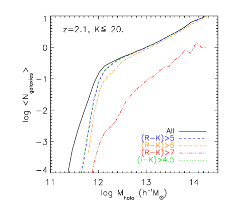
Figure 1: The HOD at $z=2.1$ of galaxies with $K\leq 20$ (solid black line) and of EROs with the same K limit and $(R-K)>5,6,7$ (dashed, dash-dotted and dash-triple dotted lines lines respectively, as indicated by the key) and $(i-K)>4.5$ (dotted line).

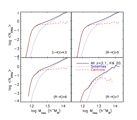
Figure 2: Solid lines show the HOD of all EROs with $K\leq 20$ at $z=2.1$. The dotted (dashed) lines show the predicted HOD for satellite (central) EROs. Different panels show the HOD predictions for EROs selected with different colour cuts, as labelled.

In Fig. 1 the predicted HOD of EROs with $K\leq 20$ at $z=2.1$ is compared with that of all galaxies with the same magnitude limit, but without any colour cut. At this redshift, the HOD of K-selected galaxies and of EROs with either $(R-K)>5$ or $(i-K)>4.5$ differ only in the low mass cutoff. As we found in Paper I, this shows that EROs with $K\leq 20$ tend not to be hosted by haloes with low masses ($M_{\rm halo}>4\times 10^{11}h^{-1}M_{\odot}$ in this case). At $z=2.1$, the cut in apparent magnitude of $K=20$, corresponds to an absolute magnitude of $M_{K}-5{\rm log}\,h\approx-25.5$ (observer frame). According to the model, this value is close to $L*$ at $z=2.1$. Thus, Fig. 1 shows the HOD of $\sim L*$ and brighter galaxies. In Paper I it was shown that in the Bower et al. model, EROs account for most of the bright end of the K-band luminosity function at $1\lesssim z\lesssim 2.5$, explaining the similar HODs predicted for EROs and for all K-selected galaxies at $z=2.1$. At lower redshifts in the ERO range, moving toward $z=1$, the difference between the ERO HOD and the overall galaxy HOD becomes larger. In this case, we are picking up less luminous galaxies and a smaller fraction of these satisfy the colour cut to be classified as EROs.

Fig. 1 shows that the HOD of all galaxies with $K\leq 20$ at $z=2.1$ is predicted to have a clear cutoff at low masses followed by an approximately power law rise. Below $M_{\rm halo}\sim 10^{12}h^{-1}M_{\odot}$, the probability of hosting an ERO is close to zero. Nevertheless, as we shall see in the next subsection, such haloes where the HOD is rising from zero can have a big influence on the predicted clustering (see Kim et al., 2009). To model this transition region accurately it is necessary to generate many examples of merger histories of such haloes, to accurately quantify the fraction that host EROs.

Fig. 1 shows that the HOD of all galaxies with $K\leq 20$ at $z=2.1$ flattens out at a value of $\langle N\rangle_{M}$ below unity, in contradiction with the expectation for the generic form of the HOD. This implies that central galaxies with these characteristics are not expected to be found in every halo. The same trend is found for EROs. Fig. 2 shows that for EROs at $z=2.1$, the HOD of central galaxies only reaches unity for haloes with $M>10^{14}h^{-1}M_{\odot}$, except in the case of EROs with $(R-K)>7$, for which a mean occupation of unity is never reached.

To understand this prediction, we examine the trend between the K-band luminosity and the host halo mass. If there was a well defined trend between the luminosity of a central galaxy and the mass of its host halo, then the central galaxies residing in haloes above a given mass would typically be brighter than some limiting magnitude. We say “typically” to allow for scatter in the relation between galaxy luminosity and halo mass. However, in the Bower et al. model, we do not find such a correlation. For low halo masses, those in which AGN suppression of gas cooling is not effective, a monotonic relation between central galaxy luminosity and halo mass is predicted, with sufficiently small scatter to make the trend clear. This relation flattens and the scatter increases substantially beyond the mass in which gas cooling is first suppressed by accretion onto the central supermassive black hole. A central galaxy of a particular luminosity can be found in a broad range of halo masses, covering several decades in mass. For models including AGN feedback, it is no longer the case that the brightest central galaxies will be found exclusively in the most massive haloes. Instead, the tails of the luminosity-halo mass relation play a critical role. We find that for the brightest galaxies, only a fraction of haloes of any mass have formation histories which can produce such an object, hence $\langle N\rangle_{M}\lesssim 1$.

Fig. 1 shows that the minimum mass, $M_{1}$, required for a halo to host two K-selected galaxies is a factor of $\sim 11$ higher than that required to host only one, which is labelled $M_{min}$. This is also the case for EROs except for those with $(R-K)>7$. In this case, haloes are predicted to host at most one ERO with $(R-K)>7$ and thus, $\langle N\rangle_{M}<2$ for all masses. The similarity in the factor found for EROs and K-selected galaxies indicates that our result is not peculiar to the additional colour selection associated with an ERO sample, but appears to be a characteristic of bright galaxies. Indeed, we note that a similar ratio $M_{1}/M_{\rm min}\sim 11$ has been suggested for local galaxies brighter than $1.1L*$, while $M_{1}/M_{\rm min}\sim 17$ for fainter galaxies (Zehavi et al., 2010).

Fig. 2 compares the predicted HOD for EROs selected with different colour cuts, separating the contributions from central and satellite galaxies. We note in Fig. 2 that the step in the HOD is less pronounced for redder central EROs. As an example, we find at $z=2.1$ an average of $0.1$ EROs with $(R-K)>5$ and $K\leq 20$ per halo with $10^{12}h^{-1}M_{\odot}$, while fewer than one in a thousand haloes host EROs with $(R-K)>7$ and $K\leq 20$ at this mass. In Paper I, we found that redder cuts select brighter and older EROs. Thus, on the one hand, the variation of the HOD with colour predicted here is in agreement with a $\langle N\rangle_{M}$ shape dominated by bright and old galaxies (Berlind et al., 2003; Zheng et al., 2005; Kim et al., 2009; Zehavi et al., 2010). On the other hand, Fig. 2 shows that the split between central and satellite galaxies varies with the colour cut used to define the ERO sample. The fraction of satellite galaxies increases for the redder cuts. The difference in the number of satellite EROs causes the shape of the halo occupation distribution to vary from a clear step function plus a power law for EROs with $(R-K)>5$ or $6$, to a distribution close to a pure power law for EROs with $(R-K)>7$. In this case, the HOD for central galaxies does not get close to unity before it is dominated by the satellite HOD.

3.2 The HOD-weighted halo mass function

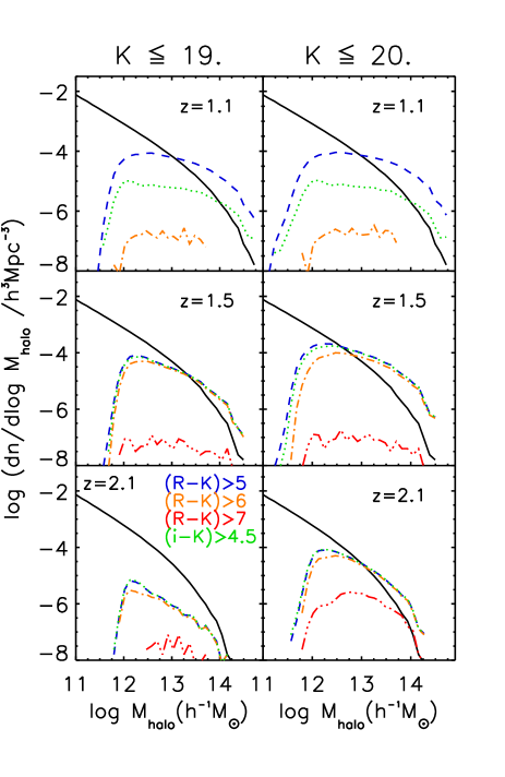
Figure 3: The mass function of all dark halos (solid lines) and the HOD-weighted halo mass function for different ERO selections. As in Fig. 1 dotted lines correspond to the mass function weighted by EROs with $(i-K)>4.5$, dashed lines to $(R-K)>5$, dash-dotted to $(R-K)>6$ and dash-triple dotted to $(R-K)>7$. Left-hand panels show the prediction for EROs with $K\leq 19$ and right-hand ones for $K\leq 20$. Top row corresponds to $z=1.1$, the middle to $z=1.5$ and the bottom row to $z=2.1$, as labelled.

The HOD by itself does not contain any explicit information about the number density of dark matter haloes. For a given redshift and assuming an initial power spectrum of matter fluctuations, the number density of halos as a function of mass, i.e, the halo mass function, depends only on the cosmology. Press & Schechter (1974) argued that for a Gaussian density field the abundance of haloes more massive than a characteristic mass is expected to decline exponentially, with a power law like behaviour at lower masses, a prediction confirmed by numerous N-body simulations (e.g. Jenkins et al., 2001). Fig. 3 shows as solid black lines the mass function of dark halos at different redshifts predicted by the Millennium Simulation.

We plot in Fig. 3 the halo mass function multiplied by the mean number of EROs per halo, where the EROs are defined with different colour cuts, $(i-K)>4.5$ and $(R-K)>5,\,6,\,7$, and in two magnitude ranges, $K\leq 19$ and $K\leq 20$. As anticipated in Paper I, we see from Fig. 3 that EROs can be found in halos with a wide range of masses. In the lowest mass bins we see a sharp cutoff driven by the shape of the HOD.

We note that a colour cut not shown in Fig. 3 but that is widely used for observationally selecting EROs is $(R-K)>5.3$. At $z=1.1,\,1.5$ and $2.1$, the HOD for EROs with $(i-K)>4.5$ is practically the same as that for EROs with $(R-K)>5.3$.

Fig. 3 shows how at $z=1.5$ and $z=2.1$ the weighted mass functions for EROs with $(i-K)>4.5$ and $(R-K)>5$ practically overlap, while they differ at $z=1.1$. For the two magnitude limits shown in Fig. 3, the predicted redshift distributions of EROs with either $(i-K)>4.5$ or $(R-K)>5$ have medians around $z=1.5$. However, the low redshift tail cuts off more sharply for EROs with $(i-K)>4.5$ and, therefore, these EROs are expected to contribute less to the mass function at $z=1.1$, explaining the difference seen in Fig. 3.

The mass of haloes such that $\langle N\rangle_{M}=1$ for EROs is given by the mass at which the HOD-weighted halo mass function has the same amplitude as the halo mass function. In Fig. 3 this happens when a line crosses the dark matter halo mass function (solid line). More massive halos will contain, on average, more than one ERO. In Fig. 3 we see that for EROs with $(R-K)>5$ and $K\leq 19$ the mass at which their $\langle N\rangle_{M}=1$ increases by a factor of $\sim 2.5$ from $z=1.1$ to $z=1.5$. Fig. 3 shows again that EROs only inhibit halos more massive than a certain threshold value, which depends on redshift, apparent magnitude limit and on colour. Both the mass at which $\langle N\rangle_{M}=1$ and the minimum mass for a halo to host an ERO increase with redshift. This trend is related to the fixed apparent magnitude limit which means that we are looking at intrinsically brighter galaxies at higher redshifts.

In contrast, the median mass of haloes hosting EROs increases with reducing redshift. For EROs with $(R-K)>5$ and $K\leq 19$ the median mass of their host haloes increases from $1.8\times 10^{12}\,h^{-1}M_{\odot}$ at $z=2.1$, to $4.4\times 10^{12}\,h^{-1}M_{\odot}$ at $z=1.1$. This increase is close to that for the dark matter $M*$. Thus, this tendency is related to the growth of dark matter haloes with time and it is seen also for EROs with $(i-K)>4.5$ and for K-selected galaxies.

We have found that brighter EROs are hosted by more massive haloes. In particular, at $z=1.5$, halos more massive than $\sim 2\times 10^{13}h^{-1}M_{\odot}$ will contain, on average, at least one ERO with $K\leq 19$, while one or more EROs with $K\leq 20$ will be present in halos with masses $\sim 5\times 10^{12}h^{-1}M_{\odot}$. Our predicted values agree with those from the empirical model of Moustakas & Somerville (2002).

In general, as shown by Fig. 3, the redder an ERO, the more massive is the typical host halo. In particular, all halos are predicted to host on average fewer than one ERO redder than $(R-K)=7$. For EROs with $K\leq 19$ at $z=1.5$, the median mass of their host haloes increases from $2.5\times 10^{12}\,h^{-1}M_{\odot}$ for EROs with $(R-K)>5$, to $6.3\times 10^{12}\,h^{-1}M_{\odot}$ for EROs with $(R-K)>7$.

We have explored the HOD-weighted mass function separating the contribution from satellite and central EROs, and find that at $z=1.1$ central EROs are rare, i.e. they make a marginal contribution to the ERO-weighted mass function for massive haloes. The average number of central EROs at $z=1.1$ is well below one per halo, even for halos as massive as $10^{14}h^{-1}M_{\odot}$. This is not the case at redshifts $z=1.5$ and $z=2.1$. At these redshifts, we find that massive haloes are expected to host an ERO as their central galaxy (except at $z=2.1$ and $K\leq 19$, in which case EROs are just rare). Thus, the increase from $z=1.5$ to $z=1.1$ in the halo mass where $\langle N\rangle_{M}=1$ for EROs with $(i-K)>4.5$, appears to be related to the fact that at lower redshifts the fraction of satellite EROs increases.

4 The two-point correlation function of EROs

In this section we present the predictions for the two-point correlation function of EROs, $\xi(r)$. The Bower et al. model is implemented in the Millennium simulation and thus, it can be used to directly predict the spatial distribution of galaxies and hence the two-point correlation function. In real-space, the Cartesian comoving co-ordinates of EROs within the simulation box are used to compute pair separations. We calculate their two-point correlation function, $\xi$, using a simple estimator (e.g. Peebles, 1980):

$$1+\xi=\frac{2DD}{n^{2}V{\rm d}V}\,,$$ (1)

where $DD$ is the number of distinct galaxy pairs with separation between $r$ and $r+{\rm d}r$ measured from the simulation, allowing for periodic boundary conditions, $n$ is the mean number density of galaxies, $V$ is the total simulated volume, and d$V$ is the volume of the spherical shell of radius $r$ and thickness d$r$. The denominator of Eq. 1 corresponds to the average number of neighbours found in d$V$ in the case of a Poisson distribution.

4.1 The shape of the two-point correlation function

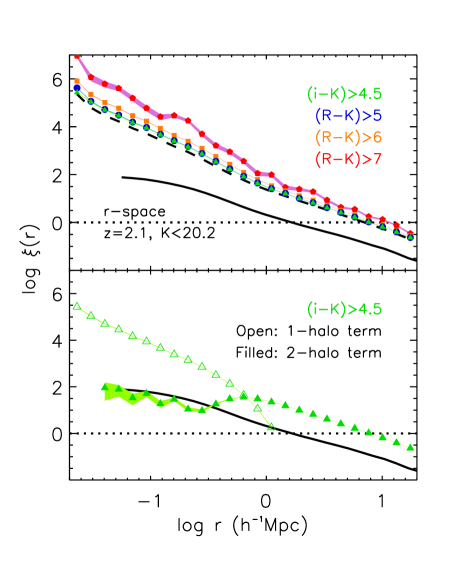
Figure 4: The predicted real-space two-point correlation function, $\xi$, at $z=2.1$, as a function of comoving separation. The upper panel shows the predicted $\xi$ for all K-selected galaxies with $K<20.2$ (dashed line), and for those which are also EROs, with $(i-K)>4.5$ (triangles), $(R-K)>5$ (circles), $6$ (squares), $7$ (pentagons). The bottom panel shows the predicted $\xi$ for EROs with $(i-K)>4.5$, distinguishing between the contributions from the one-halo term (open triangles) and the two-halo term (filled triangles; see text for details). In both panels we also show the predicted $\xi$ of the dark matter (solid line). The dotted line shows $\xi=1$ and the shaded areas show the 1$\sigma$ Poisson errors derived using the number of pairs predicted by the model at a given separation.

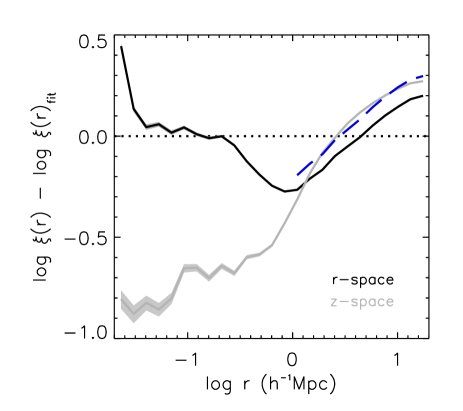
Figure 5: The predicted ratio between the spatial correlation function of EROs, with $(R-K)>5$ and $K<20.2$ at $z=2.1$, and a power law fit, $\xi_{\rm fit}=(r/r_{0})^{\gamma}$, where $r_{0}$ is $7.0\,h^{-1}{\rm Mpc}$, and $\gamma$ is $-2.1$. The solid black (grey) line corresponds to the ratio using the real (redshift) space correlation functions. The dashed line is the redshift-space clustering for $r>1h^{-1}$Mpc obtained by multiplying the clustering in real-space by the Kaiser factor (Eq. 2, §4.1.4). The shaded areas show the 1$\sigma$ Poisson errors derived from the number of pairs at a given separation.

The predicted real-space two-point correlation function at $z=2.1$ for galaxies with $K<20.2$, including EROs, is plotted in Fig. 4. This magnitude limit has been chosen to match that used in deep observational surveys (Roche et al., 2002; Miyazaki et al., 2003). The predicted shape of the two-point correlation function for all K-selected galaxies and EROs is roughly consistent with a power law for pair separations in the range $0.03\lesssim r\,\lesssim 30h^{-1}{\rm Mpc}$.

Fig. 5 plots the ratio between the correlation function of the EROs and a power law, $\xi_{\rm fit}=(r/r_{0})^{\gamma}$, of EROs with $(R-K)>5$ and $K<20.2$ at $z=2.1$. This emphasizes any deviation from a power law of the real-space correlation function. The parameters of the power law $\xi_{\rm fit}$ are those that give the best fit to the real space correlation function of the EROs plotted in Fig. 5: $r_{0}=7.0\,h^{-1}{\rm Mpc}$ and $\gamma=-2.1$. Fig. 5 shows that there is a change in slope at $r\sim 1h^{-1}{\rm Mpc}$. We have quantified this change by fixing $r_{0}$ and then fitting $\xi$ separately for $r<1h^{-1}{\rm Mpc}$ and for larger separations. We have found a change in slope $|\Delta\gamma|\leq 0.5$ (less than $25$%) between large and small scales for the case of EROs selected with different colour and K-magnitude cuts and at redshifts $z=1,\,1.5$ and $2$.

Gravitational instability theory predicts the existence of an inflection point in the two-point correlation function of dark matter when a smooth initial power spectrum is assumed, such as a power law. This occurs at the transition from the linear to the non-linear regime, which is related to the one-halo to two-halo transition (see e.g. Peebles, 1980; Gaztañaga & Juszkiewicz, 2001; Scoccimarro et al., 2001). From both semi-analytical models and smoothed particle hydrodynamics simulations, a similar change in slope is expected to occur for the two-point correlation function of galaxies, for separations close to the dark matter correlation length, $r_{0}$, i.e. the separation for which $\xi_{DM}(r_{0})=1$. The strength of the inflection depends on the galaxy selection which determines the number of galaxies per halo and the balance between the one and two halo term. This transition is supported by observations at low redshift (e.g. Baugh, 1996; Gaztañaga & Juszkiewicz, 2001; Zehavi et al., 2002). We can see such behaviour in Figs. 4 and 5. Around $1h^{-1}{\rm Mpc}$, the two-point correlation function measured for all K-selected galaxies and EROs has a small change of slope that makes the correlation function steeper on small scales.

On small scales, $r<1h^{-1}{\rm Mpc}$, $\xi$ mainly measures the number of pairs of galaxies within the same halo, i.e. the one-halo term (e.g. Benson et al., 2000b). The one-halo term is dominated by the distribution of satellites within single haloes. Thus, a sample with a higher proportion of satellites will have a boost in the clustering on small scales. The distribution of satellite galaxies depends strongly on the selection criteria (magnitude limit, colour cut, redshift range, etc.). The lower panel of Fig. 4 shows separately the contribution of the one-halo and two-halo terms to the predicted global clustering of EROs with $(i-K)>4.5$. We note that the two predicted contributions for EROs with $(R-K)>5$ are almost indistinguishable from those for EROs with $(i-K)>4.5$.

On larger scales, $r>1\,h^{-1}{\rm Mpc}$, we are generally probing the positions of galaxies in different halos, the two-halo term. We can see in the lower panel of Fig. 4 that the two-halo term of EROs has the same shape as the correlation function of the dark matter. On these scales, the two point correlation function of galaxies traces that of their host dark matter haloes scaled by their bias and the dark matter clustering is close to the prediction from linear theory on these scales. We measure the clustering of EROs with $(R-K)>5$ and $K<20.2$ at $z=2.1$, $\xi_{gg}(r)$, to be boosted with respect to that of dark matter, $\xi_{DM}$, with a bias $b\simeq\sqrt{\xi_{gg}(r)/\xi_{DM}}\sim 3$ (at $r=8h^{-1}$Mpc). This is consistent with these galaxies being hosted by haloes with $M_{halo}\sim 4\times 10^{13}h^{-1}M_{\odot}$, in agreement with the predictions shown in Fig. 3.

In the lower panel of Fig. 4 it is noticeable that the two-halo term for EROs does not go to zero at scales where the one-halo term dominates. For EROs there is a large satellite component. It is then possible for two haloes that are almost touching, to have satellite pairs at a smaller separation than that corresponding to the centres of the two haloes.

4.1.1 Variation of clustering with colour

Fig. 4 shows that at $z=2.1$ galaxies in the ERO samples defined by the bluest cuts, with $(R-K)>5$ or $(i-K)>4.5$, cluster in a very similar way. In line with the results described in §3, the clustering of these bluest EROs is also seen to be very close to that of galaxies selected solely on the basis of their K-band apparent magnitude without a cut in colour. EROs with $(R-K)>5$ or $(i-K)>4.5$ account for most of the bright end of the luminosity function of K-selected galaxies at $z=2.1$, which explains their similar clustering.

Fig. 4 also shows that the reddest EROs display the strongest change in power law slope with pair separation. As discussed above, a larger proportion of satellite galaxies is found among the redder EROs, explaining the boost seen at small scales.

4.1.2 Variation of clustering with redshift

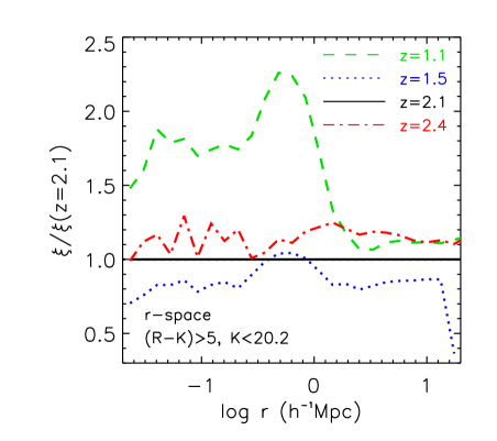
Figure 6: Variation with redshift of the predicted real-space two-point correlation function for EROs with $(R-K)>5$ and $K<20.2$. Correlation functions at $z=1.1,\,1.5,\,2.1,\,2.4$ (dashed, dotted, solid and dash-dotted line, respectively) are shown divided by the correlation function predicted at $z=2.1$.

Table 1: The predicted real-space comoving correlation length, $r_{0}$, for EROs with $(R-K)>5$ and different magnitude cuts, at $z=1.1,\,1.5,\,2.1$. Not enough EROs with $K<18.4$ are found at $z=2.1$ to have an estimation of their clustering.

		$r_{0}(h^{-1}{\rm Mpc})$
$z$	$K<20.2$	$K<19.2$	$K<18.4$
1.1	8.4	8.1	7.5
1.5	7.2	7.3	7.2
2.1	7.9	7.3	-

Table 1 presents the real-space comoving correlation length, $r_{0}$, of EROs with $(R-K)>5$ for different redshifts and magnitude ranges. The correlation length is obtained here as the galaxy separation that gives $\xi(r_{0})=1$.

In Table 1 we can see that $r_{0}$ does not change monotonically with redshift. This lack of a clear evolutionary trend has also been found observationally by Brown et al. (2005). A similar prediction was made from the theoretical predictions in Baugh et al. (1999) for a sample with a fixed apparent magnitude limit, so this trend is not necessarily peculiar to the colour selection.

The variation of the clustering of EROs with redshift is small. Therefore, we have emphasized this variation by presenting in Fig. 6 the clustering of EROs with $(R-K)>5$ and $K<20.2$ at different redshifts, $z=1.1,\,1.5,\,2.1$ and $2.4$, divided by that at $z=2.1$. It is clear from Fig. 6 that the two-point correlation function of EROs in real-space presents a slightly different shape at $z=1.1$ than at higher redshifts, showing a boost on small scales $r\lesssim 0.5h^{-1}{\rm Mpc}$. This is related to the higher fraction of satellite galaxies selected at $z=1.1$ as EROs, in comparison with the higher redshifts plotted, as reported in §3.

The evolution of the correlation function with redshift is important for interpreting the angular clustering of galaxies. This evolution is often parametrised as a global, scale independent factor in redshift. Fig. 6 shows that the variation of the clustering with redshift is different on large and small scales. This makes it difficult to assign a unique redshift power law, $1/(1+z)^{\alpha}$, to describe this evolution, so such “deprojections” of angular clustering are at best approximate.

4.1.3 Variation of clustering with apparent magnitude

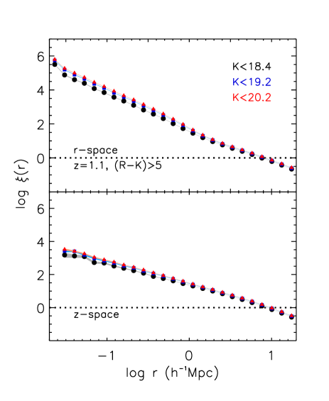
Figure 7: The predicted spatial two-point correlation function of EROs, with $(R-K)>5$, brighter than $K<18.4$ (circles), $19.2$ (squares), $20.2$ (triangles) at $z=1.1$. The real-space prediction is shown in the upper panel and the redshift-space in the bottom. In both cases, the shaded areas show the 1$\sigma$ Poisson errors, derived using the number of pairs predicted at a given comoving separation.

Fig. 7 shows the predicted two-point correlation function at $z=1.1$ in both real and redshift-space for EROs with $(R-K)>5$ and $K<18.4,\,19.2$ and $20.2$. At this redshift, the model predicts the existence of EROs in sufficient numbers for each of these magnitude cuts to allow as to compare the clustering characteristics. We find that the clustering of EROs depends weakly on luminosity. Fainter EROs are predicted to be slightly more clustered than brighter ones, due to a higher fraction of satellite galaxies in massive haloes. Fig. 7 shows that the strongest variation occurs on small scales. Table 1 also shows a weak trend for fainter galaxies to have a higher comoving correlation length, $r_{0}$.

Table 1 lists the predicted $r_{0}$ for EROs selected in magnitude ranges similar to various observational studies that inferred the correlation length by fitting models to the measured angular correlation functions. Daddi et al. (2001) analysed $400$ EROs with $K_{S}<19.2$, $(R-K_{S})>5$ and a median redshift $z\sim 1.2$ in a $701\,{\rm arcmin}^{2}$ field and estimated that their correlation length is not less than $r_{0}=8h^{-1}$Mpc, with a most probable estimate of $r_{0}\sim 12\pm 3h^{-1}{\rm Mpc}$. Roche et al. (2002) inferred that EROs with $K<20.2$, $(R-K)>5$ and $1\leq z_{\rm photo}\leq 3$ ($158$ EROs in a $81.5\,{\rm arcmin}^{2}$ field), have a correlation length between $10h^{-1}$Mpc and $13h^{-1}$Mpc. Brown et al. (2005) inferred the correlation length of EROs with $K<18.4$, $(R-K)>5$ and a median photometric redshift of $z\sim 1.2$ ($671$ EROs in a $3529\,{\rm arcmin}^{2}$ field), to be $9.7\pm 1.0\,h^{-1}{\rm Mpc}$.

Table 1 shows that the predicted correlation length for EROs is consistently lower than that estimated from the observations. However, the predicted correlation length for EROs with $K<19.2$ at $z=1.1$ is above the lower limit estimated by Daddi et al. (2001) and within the $2\sigma$ range of their best estimate of $r_{0}$. The comparison with correlation lengths deduced from observations is not ideal since a number of assumptions have to be made to infer this quantity from the actual observables. In particular, all the observational studies mentioned above assumed a power law for the spatial two-point correlation function, $\xi$, with a fixed index $\gamma\approx-1.8$. The predicted $\xi$ is best fitted by a power law with an index $\gamma\approx-2.1$ at $z=1.1$ and at $z=2.1$, as shown at the beginning of §4.1. Thus, if this predicted value was adopted for the observational estimation, lower correlation lengths would be obtained, resulting in a better agreement between the model and observations. A direct comparison with the observed two-point angular correlation function will be carried out in §5.

4.1.4 Clustering in real and redshift-space

To mimic a spectroscopic survey in which radial positions of galaxies are inferred from their redshifts, galaxy positions are perturbed along one of the axes by their peculiar velocities, scaled by the appropriate value of the Hubble parameter. The impact of these peculiar motions depends on the scale. Figs. 5 and 7 show that while the slight change of slope around $1h^{-1}$Mpc in the correlation function of EROs is clear in real space, this is smeared out when including redshift-space distortions.

Fig. 5 emphasizes the differences between the correlation functions in real and redshift-space by plotting the correlation functions divided by the power law that best fits the real-space clustering of EROs. Both Figs. 5 and 7 show that the difference between real and redshift-space clustering depends on scale.

On small scales, $r\lesssim 1h^{-1}{\rm Mpc}$, the clustering in redshift-space is significantly lower than that in real space. On these scales we are generally considering galaxies within the same halo. As can be seen in Fig. 3, the Bower et al. model predicts the existence of more than one ERO in halos of high enough mass, except for the most extreme EROs with $(R-K)>7$. The peculiar motions of EROs within a halo cause an apparent stretching of the structure in redshift-space, diluting the number of ERO pairs at small separations. Thus, the correlation function signal measured in redshift-space is smaller than that in real-space on these scales.

On larger scales, $1\lesssim r\lesssim 30h^{-1}{\rm Mpc}$, bulk motions of galaxies cause the galaxy distribution to appear squashed along the line of sight in redshift-space, enhancing the clustering amplitude. Fig. 5 shows that, on this range of scales, the boost measured for the redshift-space correlation function is in reasonable agreement with the value expected according to the formalism developed by Kaiser (1987). This relates the correlation function in redshift-space, $\xi_{gg}(s)$, to that in real-space, $\xi_{gg}(r)$, through a factor, $f$, $\xi_{gg}(s)=f\xi_{gg}(r)$. This factor is a function of the bias, $b$, and the matter content of the Universe, $\Omega_{m}$:

$$f=1+\frac{2}{3}\frac{\Omega_{m}^{\gamma^{\prime}}}{b}+\frac{1}{5}\Big{(}\frac{\Omega_{m}^{\gamma^{\prime}}}{b}\Big{)}^{2}$$ (2)

In fact, the redshift-space clustering is only expected to be accurately described by the “Kaiser factor” on very large scales, since linear perturbation theory is assumed (Jennings et al., 2011). Traditionally $\gamma^{\prime}=0.6$ but $\gamma^{\prime}=0.55$ is a better approximation (Linder, 2005) and is the value we have used here.

4.2 Clustering of quiescent and star forming EROs

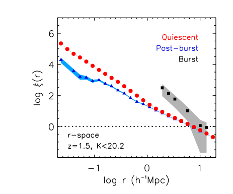
Figure 8: The predicted real-space two-point correlation function for EROs with $(R-K)>5$ and $K<20.2$ at $z=1.5$, separated into burst (squares), post-burst (triangles) and quiescent (circles) galaxies (see text in §4.2 for details).

Observationally, EROs exhibit a mixture of spectral properties which are related to their star formation histories and dust content. In this section we analyse the differences in the predicted clustering between EROs that are actively forming stars and those that are passively evolving.

Fig. 8 shows the clustering of EROs with $(R-K)>5$ and $K<20.2$ at $z=1.5$, divided into burst (galaxies with an ongoing burst of star formation), post-burst (last burst happened within the past 1 Gyr) and quiescent galaxies (all the others). As described in Paper I, this classification is made by considering the lookback time to the start of the last burst of star formation experienced by the galaxy. In the Bower et al. model bursts are triggered by galaxy mergers and by disks becoming dynamically unstable.

The higher clustering amplitude predicted in real-space for burst EROs, $r_{0}=11.7h^{-1}{\rm Mpc}$, is noticeable compared with that of quiescent ones, for which $r_{0}=7.3h^{-1}{\rm Mpc}$, and for post-burst ones, with $r_{0}=6.7h^{-1}{\rm Mpc}$. However, Poisson errors dominate the burst ERO clustering estimate, due to the much lower space density of these EROs compared with the other two samples. We can see in Fig. 8 how the correlation functions for quiescent and post-burst EROs are similar for separations larger than $r\sim 1h^{-1}{\rm Mpc}$, with slopes differing by $|\Delta\gamma|<0.2$ on small scales. The same tendencies are found in redshift-space.

In Paper I, we explored the predicted mix of quiescent and active EROs using different classifications. In particular, we used the colour-colour diagram proposed by Pozzetti & Mannucci (2000), the specific star formation rate of EROs, adopting $SFR/M_{*}=10^{-11}{\rm yr}^{-1}$ as the boundary, and the classification described above, but considering as active both post-burst and burst EROs. We found that the number counts of quiescent EROs agreed among the different classifications. $75$% of the quiescent EROs in Fig. 8 have $SFR/M_{*}<10^{-11}{\rm yr}^{-1}$. We find that the EROs with $SFR/M_{*}<10^{-11}{\rm yr}^{-1}$ have a correlation length $r_{0}=7.7h^{-1}{\rm Mpc}$ and that, globally, their two-point correlation function is very close to that for quiescent EROs. The correlation lenght of EROs with $SFR/M_{*}>10^{-11}{\rm yr}^{-1}$ is predicted to be $r_{0}=5.7h^{-1}{\rm Mpc}$, slightly lower than that for post-burst EROs.

The active EROs, post-burst plus burst EROs, are dominated in our model by the post-burst galaxies. The predicted clustering of active EROs practically overlaps with that for post-burst EROs only, having the same predicted correlation length $r_{0}=6.7h^{-1}{\rm Mpc}$.

A few observational studies have tried to obtain the real-space correlation length differentiating between quiescent EROs and dusty star forming or active EROs. Among these are those by Daddi et al. (2002) and Miyazaki et al. (2003) studies, which inferred the correlation length of EROs from the measured angular clustering.

Miyazaki et al. (2003) observed EROs with $(R-K_{S})>5$ and $K_{S}<20.2$, dividing the sample into quiescent and star forming galaxies by fitting observed broad band colours to synthetic spectral energy distributions. Without taking into account the photometric redshift errors, Miyazaki et al. found the correlation functions of quiescent and active EROs to be $r_{0}=11\,\pm\,1\,h^{-1}$Mpc and $r_{0}=12\,\pm\,2\,h^{-1}$Mpc, respectively. In agreement with the observations of Miyazaki et al., we find that quiescent and active EROs have similar correlation lengths. Taking into account the photometric redshift errors, Miyazaki et al. revised their estimate of the correlation length for quiescent EROs to be $r_{0}=8h^{-1}$Mpc. This value is comparable to but higher than the predicted correlation length of quiescent EROs with $(R-K)>5$ and $K<20.2$ at $z=1.5$.

Daddi et al. (2002) observed EROs with $(R-K_{S})>5$ and $K_{S}<19.2$, splitting the sample using spectral features. Daddi et al. estimated the correlation length to be $r_{0}<2.5\,h^{-1}{\rm Mpc}$ for star forming EROs and $5.5\lesssim r_{0}\lesssim 16\,h^{-1}{\rm Mpc}$ for quiescent EROs. Our predicted $r_{0}$ values for quiescent EROs agree within errors with those from Daddi et al.. The correlation function for quiescent EROs inferred by Miyazaki et al. (2003) agrees with the estimate by Daddi et al. (2002), though they used different magnitude cuts. However, these two observational studies estimated very different correlation lengths for star forming EROs. Sample variance could be responsible, at least partly, for the difference between the observational studies, since Daddi et al. covered a field $7$ times larger than that used in the Miyazaki et al. study. Another issue that will increase the discrepancy is the different depths of the two observations. Cimatti et al. (2002c) observed that star forming EROs appear at slightly higher redshifts than old EROs. This implies that surveys sampling only bright galaxies will contain a lower percentage of star forming EROs. The need for more fields to be explored observationally is clear, in order to have a better knowledge of the origin of such different $r_{0}$ values for active EROs.

5 The two-point angular correlation function of EROs

In order to make a direct comparison with current measurements of clustering, we study here the predicted angular correlation function $\omega(\theta)$ for EROs, obtained from our previous estimate of the two-point spatial correlation function in real space and the redshift distribution of model EROs.

The Limber equation (Limber, 1954) relates the spatial correlation function $\xi$ to the angular correlation function $\omega$, under the assumptions:

1. We can apply a sample selection and measure the correlation function for that full sample, without any concern for dependencies of clustering on intrinsic galaxy properties which vary within the sample (e.g. Peebles, 1980).

2. The selection function does not vary over the pair separations on which we can measure a signal for $\xi$ (see e.g. Simon, 2007). For most surveys this is a reasonable assumption, since the signal for $\xi$ will be measurable only for those pairs of galaxies such that their pair separations $|r_{1}-r_{2}|$ are much smaller than their comoving distances, $r_{1}$, $r_{2}$.

The above approximations are both reasonable for EROs. Therefore, for a flat Universe we can calculate the angular correlation function, $\omega$, for pairs of EROs separated by an angle $\theta$ by:

$$\omega(\theta)=\frac{2\int_{0}^{\infty}\Big{[}\frac{{\rm d}N}{{\rm d}z}\Big{]}^{2}\frac{{\rm d}z}{{\rm d}r}\,\Big{(}\int_{0}^{2r}{\rm d}u\,\xi(r_{12},z)\Big{)}\,{\rm d}z}{\Big{[}\int_{0}^{\infty}\frac{{\rm d}N}{{\rm d}z}\,{\rm d}z\Big{]}^{2}}\,,$$ (3)

where d$N/{\rm d}z$ is the redshift distribution of the surveyed galaxies. For a pair of galaxies at comoving distances $r_{1}$ and $r_{2}$: $u=r_{1}-r_{2}$, $r=(r_{1}+r_{2})/2$ and the comoving separation between them is approximated by $r_{12}=\sqrt{u^{2}+r^{2}\varpi^{2}}$, with $\varpi^{2}=2({\rm cos}\theta-1)$. The variation of redshift with comoving distance d$z/{\rm d}r=(H_{0}/c)\sqrt{\Omega_{0}(1+z)^{3}+(1-\Omega_{0})}$, where $H_{0}$ is the Hubble constant now and $c$ is the speed of light. When integrating the two-point correlation function at very large scales, beyond those modelled accurately within the simulation volume, we assume that on these scales $\xi$ is given by a scaled dark matter two-point correlation function calculated from the linear initial power spectrum of density fluctuations, where the scaling is the linear bias factor, $b^{2}$ (see Orsi et al., 2008).

5.1 EROs selected on (R-K) colour

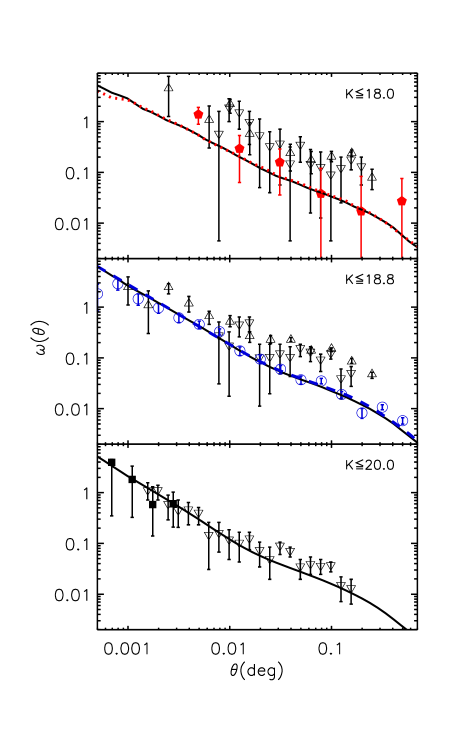
Figure 9: The two-point angular correlation function of EROs with $(R-K)>5$ and brighter than $K=18,\,18.8,\,20$, from top to bottom. The black solid lines show the predicted angular correlation. The top panel also contains a dotted line with the clustering predicted for EROs with $K\leq 17.9$. The middle panel includes a dashed line showing the predicted angular clustering for EROs with $(r-K)>5$ and $K\leq 18.8$. In each panel there are observational results for the corresponding EROs: Daddi et al. (2000b) (triangles), Roche et al. (2002) (filled squares), Brown et al. (2005) (filled pentagons), Kong et al. (2006) (upside down triangles), Kim et al. (2011) (circles). Error bars are Poisson error bars, except for the data points from Brown et al. (2005), which include the effects of sample variance and shot noise.

Fig. 9 shows the predicted $w(\theta)$ for EROs with $(R-K)>5$ and different apparent magnitude cuts, compared with observations. The triangles in Fig. 9 show the clustering of EROs studied by Daddi et al. (2000b) in a field, Daddi-F, which covers $701\,{\rm arcmin}^{2}$ and is $85$% complete to $K_{S}<18.8$. The upside down triangles in Fig. 9 show the clustering of EROs studied by Kong et al. (2006) in both a subsection of the Daddi-F field of $600\,{\rm arcmin}^{2}$ and in the Deep3a-F field with an area of $320\,{\rm arcmin}^{2}$. The squares in Fig. 9 show the clustering of EROs measured by Roche et al. (2002) in a $81.5\,{\rm arcmin}^{2}$ field. The pentagons in Fig. 9 show the clustering of EROs with $K<17.9$ measured by Brown et al. (2005) in a $0.98\,{\rm deg}^{2}$ field; their error estimate uses a Gaussian approximation to the covariance matrix and, thus, includes the effects of sample variance and shot noise. Kim et al. (2011) measured the clustering of EROs with $(r-K)>5$ and $K\leq 18.8$ observed in the SA22 field with an area of $2.45\,{\rm deg}^{2}$, one of the largest fields used to date to measure ERO clustering. The Kim et al. (2011) data points are shown as open circles in Fig. 9

Both Daddi et al. (2000b) and Kong et al. (2006) observed roughly the same field using different R-filters. Their estimates of the clustering of EROs agree within the errors, though Kong et al. (2006) measured a slightly higher clustering amplitude than Daddi et al.

The top panel in Fig. 9 shows the predicted angular clustering of EROs for both $K\leq 18$, solid line, and $K\leq 17.9$, dotted line, to match the observational samples. The predicted difference is minimal, as expected for such a small change in magnitude. The top panel in Fig. 9 shows that the model reproduces the clustering estimated by Brown et al. (2005) for EROs with $K\leq 17.9$ in a field $5$ times larger than that observed by Daddi et al. (2000b) and Kong et al. (2006) (Daddi-F field).

The middle panel in Fig. 9 shows the predicted angular clustering of EROs with $K\leq 18.8$ compared with the estimates from Daddi et al. (2000b), Kong et al. (2006) and Kim et al. (2011). As we found for brighter EROs, our predicted angular clustering is lower than that estimated by both Daddi et al. and Kong et al. (Deep3a-F field). However, it is clear from Fig. 9 that the model predictions match the clustering for EROs with $K\leq 18.8$ estimated by the UKIDSS team (Kim et al., 2011) over an area $12$ times larger than the Daddi-F field. The middle panel in Fig. 9 also shows the predicted angular clustering for EROs selected with $(r-K)>5$, the same filters used by Kim et al. (2011). Both $r$ and $R$ filters are very close, and the difference in the predicted angular clustering is negligible.

For EROs with $(R-K)>5$ and $K\leq 20$, the bottom panel of Fig. 9 shows that the predicted clustering reproduces the observational estimates from both Roche et al. (2002) and Kong et al. (2006) (Deep3a-F field). This is also true for EROs with $K\leq 19.5$.

Kong et al. (2006) found an increase in the amplitude of the angular correlation function with the brightness of EROs. The observed variation of clustering with magnitude is stronger than that predicted, even after taking into account some small discrepancies due to the use of slightly different filters. This is not peculiar to EROs, since a similar conclusion was reached by Kim et al. (2010), who studied bright galaxies at $z=0$, finding that the clustering predicted by semi-analytical models does not vary with luminosity as strongly as observed. Kim et al. (2010) concluded that a stronger dependence of clustering strength on luminosity could be obtained by including additional physical processes which influence the mass of satellite galaxies. This could have an implication for EROs as an appreciable fraction of our EROs are satellites.

Nevertheless, once the sampling variance is taken into account, the model predictions do match the observed angular clustering reasonably well for $0.0006\leq\,\theta({\rm deg})\,\leq 0.6$.

5.2 EROs selected on (i-K) colour

Accurate measurements of the clustering of EROs can only be achieved by deep imaging of large areas. Currently, the UKIDSS survey (Kim et al., 2011) is one of the few surveys that has been able to measure the clustering of EROs beyond separations of $0.1$ deg (which corresponds to $\sim 2\,h^{-1}{\rm Mpc}$ at $z=1.5$), which probes the two-halo component of the correlation function. In this section we show the model predictions for EROs selected in a similar way to that adopted by Kim et al. (2011), i.e. using the $(i-K)>4.5$ colour criterion. This criterion appears to select galaxies with $z\geq 1$, with fewer lower redshift contaminants than the $(R-K)$ colour criterion (Kong et al., 2009).

5.2.1 Number counts and redshift distribution

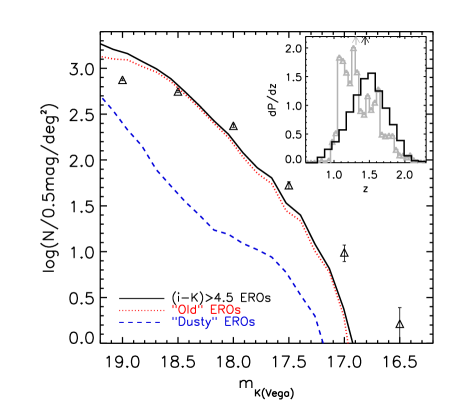
Figure 10: Differential number counts of EROs with $(i-K)>4.5$. The predicted number counts for all EROs are shown by a solid line. The prediction for “old” (“dusty”) EROs are presented with dotted (dashed) lines (see §5.2.3 for details on this division). The triangles show the observations from Kim et al. (2011), which are complete up to $K\leq 18.8$. The inset shows the redshift distribution for EROs with $(i-K)>4.5$ and $K\leq 18.8$: predictions are in black and observations in grey. The areas of the histograms are normalised to unity. The median redshifts are shown by the vertical arrows.

The success of a model in reproducing the observed angular clustering of a certain type of galaxy is more robust if the model also reproduces their number density. Here we explore the predicted number counts and redshift distributions for EROs selected by their $(i-K)$ colours. We already showed the predicted abundance and redshift distributions for $(R-K)$ selected EROs in Paper I.

Fig. 10 shows the predicted differential number counts for EROs with $(i-K)>4.5$, compared with the observations from Kim et al. (2011). These observations are complete for galaxies with $K\leq 18.8$ (see Kim et al., 2011, for further details). The model underpredicts the number counts at the bright end, but gives a good match from $K=18$ to the completeness limit.

The inset in Fig. 10 shows the predicted redshift distribution of EROs with $(i-K)>4.5$ and $K\leq 18.8$. For comparison we have included, in grey, the redshift distribution estimated by Kim et al. (2011). This estimate is based on photometric redshifts measured by the NEWFIRM Medium Band Survey (Brammer et al., 2009; van Dokkum et al., 2010). The area sampled by the NEWFIRM survey is rather small, $0.25\,{\rm deg}^{2}$, and so is subject to significant sample variance, with the result that distinctive features appear in the redshift distribution. The model predicts a redshift distribution close to the observed one, but with a slightly higher median redshift $z=1.44$, as opposed to a median of $z=1.31$ for the observational data.

The model predicts a population of EROs defined with $(i-K)$ colours that is close enough in number and redshift distribution to the observations to make it worthwhile to continue calculating their clustering properties. For this purpose, we will follow the method described above for EROs selected based on their $(R-K)$ colour.

5.2.2 Angular clustering

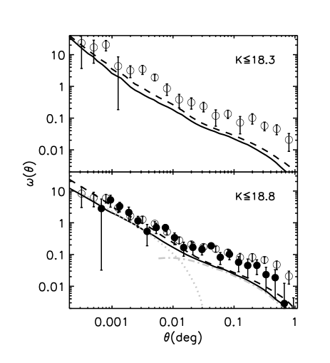
Figure 11: The predicted two-point angular correlation function of EROs with $(i-K)>4.5$ and $K\leq 18.3$ in the top panel, $K\leq 18.8$ in the bottom panel. The solid black lines show the prediction from the model. The dashed black lines show the model predictions using the observationally estimated redshift distribution from Kim et al. (2011). The grey lines in the bottom panel present the predicted contribution of the one halo (dotted line) and two halo terms (dash-dotted line). Observational results from Kim et al. (2011) for the UKIDSS DXS SA22 field are shown as open circles. The filled circles present the observational estimation for the UKIDSS Elais-N1 field (Kim et al. in preparation, 2011). Observational data points are shown with Jackknife error bars.

Fig. 11 shows the predicted two-point angular correlation function of EROs with $(i-K)>4.5$ compared with the observed angular correlation function measured within two UKIDSS fields: SA22 (Kim et al., 2011), open circles, with an area of $2.45\,{\rm deg}^{2}$ and Elais-N1, filled circles (Kim et al. in preparation, 2011) with an area of $3.88\,{\rm deg}^{2}$ (both quoted areas are after masking). The SA22 field was observed with both the CTIO and UKIRT telescopes, while the Elais-N1 field was observed with the Subaru and UKIRT telescopes. The observed correlation function in both fields is corrected for the integral constraint. For the Elais-N1 field the integral constraint is estimated to be $0.0073$, which is comparable to the clustering signal at scales of $\approx 0.7$ deg. For the clustering in both fields Jackknife errors have been estimated following Sawangwit et al. (2009), in an attempt to take into account the sampling variance (Norberg et al., 2009).

We predict the angular clustering using Limber’s equation (Eq. 3), assuming either the predicted (solid lines) or the observed (dashed lines) redshift distribution for the galaxies under study. We can see from Fig. 11 that the difference between using the predicted and observed redshift distributions is negligible. The evolution with redshift of the spatial two-point correlation function for EROs is modest, which explains the small variation seen for the angular clustering when using a different redshift distribution.

From the Kim et al. (2011) observations, the correlation function of EROs selected with $(i-K)>4.5$ appears to be better described by two power laws, rather than one, with the change of slope happening at $\theta\sim 0.02\,{\rm deg}$. The model also predicts such a change in slope, though this is milder than observed. The bottom panel in Fig. 11 shows how this change in slope is due to the change from counting pairs of galaxies within the same halo, the one halo term, to counting those from different haloes, the two halo term, as was also seen for the spatial correlation function in §4. At scales larger than $\theta\geq 0.2$ deg we can see the change in the curvature of $\omega(\theta)$ intrinsic to the two-halo term, that follows the shape of the dark matter clustering.

Fig. 11 shows that the model underpredicts the angular clustering with respect to observations. The difference becomes larger at larger pair separations beyond $\theta=0.02\,{\rm deg}$. However, as can be seen in Fig. 11, the uncertainty due to sampling variance also increases with pair separation, where the clustering measured in the two fields shows the largest differences.

As indicated before, the differences between model predictions and observations are not due to the differences in the redshift distributions. Sampling variance could be behind the discrepancy between observations and model predictions, at least at small scales, $\theta<0.02\,{\rm deg}$. On larger scales the difference is clear even when allowing for the sampling variance errors in observations of different fields. On large scales, $\theta>0.02\,{\rm deg}$, the angular clustering is underpredicted by a factor of 3 for EROs with $K\leq 18.8$.

The match between predictions and observations is worse for EROs selected with $(i-K)$ colour than it is for $(R-K)$ colours. The photometric errors in the CTIO i-filter are larger than those for the r-filter, which implies that the selection made using $(i-K)$ is slightly noisier than with $(r-K)$, at least for the SA22 field. In fact, the prediction for EROs with $(i-K)>4.5$ perfectly matches the angular clustering estimated from observations of EROs selected with $(i-K)>4$, potentially pointing towards a problem specific to the colour cut. The predicted angular clustering using the Subaru i-band is almost identical to that shown in Fig. 11. We have further explored the origin of this discrepancy by predicting the angular clustering of EROs with $(i-K)>5$. We find a similar trend to that reported for the spatial clustering: the clustering of redder EROs is boosted, with the larger variation seen at small scales. In line with this prediction, both Daddi et al. (2000b) and Kim et al. (2011) observed that redder EROs have angular correlation functions with higher amplitudes.

Optical colours in the model are affected by the treatment of the ram-pressure stripping in satellite galaxies (Font et al., 2008). When selecting EROs by their $(i-K)$ or $(R-K)$ colours we could be enhancing their numbers by selecting satellite galaxies that are redder than they should be due to an oversimplification of their gas physics in the Bower et al. model. This would change the amplitude of the angular clustering, particularly at small scales. We have investigated this point by calculating the angular clustering of EROs using the Font et al. (2008) model. This model is an extension to that of Bower et al. which introduces a more realistic treatment of the stripping of hot gas in satellite galaxies. Font et al. also double the stellar heavy element yield, improving the match of the locus of the red sequence to observational data at $z\approx 0$.

Using the Font et al. (2008) model we find that the number counts of EROs with $(i-K)>4.5$ are overpredicted for $K<18$ by around a factor of two. The redshift distribution of EROs predicted by the Font et al. model has a non negligible fraction of galaxies at $z<1$, with a median redshift of $1.13$, below that observed. At a given redshift, the spatial correlation function predicted by the Font et al. model is very close to that predicted from the Bower et al. model, for EROs with either $(i-K)>4.5$ or $(R-K)>5$. However, the angular clustering calculated from the Font et al. model is predicted to be boosted by at most a factor of $\sim 1.5$ at large scales, when compared with that from the Bower et al. model. Therefore, the Font et al. model does not reconcile the predictions with the observational estimates. Since the Font et al. model includes changes in both the stellar yield and the treatment of hot gas stripping that have opposite effects on galaxy colours, we have run the Bower et al. model changing only the stellar yield to double the original value. The results of doing this exercise are similar to using the full Font et al. model. Both the redshift distribution and number counts change upon changing the yield. These changes are such that the angular clustering remains close to that obtained with the original model. Thus, we find that a change in stellar yield cannot account for the difference between the model predictions and the observations, and leads to some predictions actually agreeing worse with the observations.

5.2.3 “Old” and “dusty” EROs with $(i-K)>4.5$

The number counts for EROs separated into “old” and “dusty” galaxies are shown in Fig. 10. This separation has been done according to the location of the EROs in the colour-colour diagram proposed by Fang et al. (2009), where the line $(J-K)\,=\,0.20(i-K)\,+\,1.08$ is defined to set the boundary between these types. This selection is similar to that of Pozzetti & Mannucci (2000), but is tuned to the filters used to select EROs with $(i-K)$ colours. Fang et al. (2009) compared EROs selected with both this colour-colour selection criterion and on the basis of their spectra, finding that the two methods agree reasonably well. Nevertheless, according to Fang et al., $\sim 33$% of the “old” EROs selected by the colour-colour method are actually young EROs when looking to their spectra.

We find that about $90$% of the EROs with $K\leq 19$ are “old” galaxies according to the Fang et al. colour criterion. We have tested that a small shift of about $6$% in the boundary proposed by Fang et al., $(J-K)\,=\,0.20(i-K)\,+\,1.02$, produces a similar change in the percentage of “old” EROs of a $5$%. Thus, the colour-colour separation is reasonably robust for the predicted EROs, since they do not preferentially populate the region close the colour-colour boundary.

Kim et al. (2011) observed that $60$% of their EROs are “old” galaxies, a lower fraction than the model predicts. This result is similar to the conclusion from Paper I on the nature of EROs selected using $(R-K)$ colours, although, in the case of the $(i-K)$ selection the difference with observations is larger. One possible reason for this discrepancy is that although galform broadly reproduces the observed colour bimodality observed for SDSS galaxies at $z=0$ (González et al., 2009), the model predictions are different in detail from the observations. However, we have found that when using either the Font et al. (2008) model or the Bower et al. model with twice the original yield value, about $60$% or $67$%, respectively, of the predicted EROs with $K\approx 18$ are “old”, in good agreement with observations. Therefore, the difference in the split between “dusty” and “old” EROs appears to be connected with the value of the yield in the Bower et al. model.

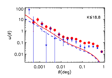
Figure 12: The predicted two-point angular correlation function of “old” (red solid line) and “dusty” (blue dashed line) EROs with $(i-K)>4.5$ and $K=18.8$. The observational estimates of Kim et al. (2011) for “old” (circles) and “dusty” (stars) EROs are shown with Poisson error bars. See text for the details of the division between “old” and “dusty” EROs.

Fig. 10 shows that the percentage of “old” EROs starts to drop for fainter magnitude bins. The same tendency has been observed by Kim et al. (2011). Kong et al. (2009) also found the same trend for a sample of EROs selected with $(I-K_{S})>4$ and $K_{S}\leq 19.2$.

The predicted median redshifts for “old” and “dusty” EROs are $1.44$ and $1.25$, respectively. Kim et al. (2011) estimated the median redshifts for the observed “old” and “dusty” EROs to be $z=1.36$ ($10$% and $90$% percentiles: $z=1.1$ and $z=1.7$, respectively) and $z=1.25$ ($10$% and $90$% percentiles: $z=1$ and $z=1.8$, respectively), respectively, in reasonable agreement with the model predictions. Contrary to these results, Fang et al. (2009) and Kong et al. (2009) found more “dusty” EROs at higher redshifts. However, we have found that this statement is strongly dependent on the particular $(i-K)$ cut made, since when using $(i-K)>5$ we find that “dusty” EROs are predicted to appear at higher redshifts than “old” ones.

Fig. 12 shows the predicted two-point angular correlation function of EROs with $(i-K)>4.5$ separated into “old” and “dusty” galaxies. Fig. 12 shows that the predicted clustering for both types of EROs differ only on small scales. Thus, model predictions and observations agree in that both “dusty” and “old” EROs are clustered very similarly.

In the previous section we discussed the possible origin of the difference between the predicted and the observed angular clustering for EROs with $(i-K)>4.5$. The balance between “dusty” and “old” EROs when using $(i-K)$ colours could alter the predicted angular clustering. However, Fig. 12 shows that the clustering of “dusty” EROs is both observed and predicted to be similar, though slightly less strong than that for the “old” EROs. Therefore, a larger fraction of “dusty” EROs within the model would actually slightly increase the difference between observations and model predictions, by further reducing the predicted angular clustering at large scales.

6 Conclusions

In this paper we have extended the tests of the galform galaxy formation model by continuing the study of Extremely Red Objects (EROs) started with Gonzalez-Perez et al. (2009) (Paper I). EROs are massive, red galaxies at $0.7\lesssim z\lesssim 3$ and their numbers and properties have posed a challenge to hierarchical galaxy formation models. In this paper we have analysed the halo occupation distribution (HOD) and clustering of EROs predicted based on the published model of galaxy formation of Bower et al. (2006). The parameters in this model were set to reproduce observations of the local galaxy population. No parameter has been changed for the work presented here. The Bower et al. model gives an impressively close match to the number counts of EROs (Paper I). This model also matches the evolution of the K-band luminosity function and the inferred evolution of the stellar mass function.

The HOD predicted by the Bower et al. model has a strikingly different form from the canonical assumption of a step function that reaches unity for the central galaxies plus a power law for satellites. The central galaxy HOD has a somewhat more rounded form than a step function and does not reach unity for K-selected galaxies or EROs. This is due to the non-monotonic relation between host halo mass and central galaxies luminosity. According to the Bower et al. model, at $z=2.1$, galaxies with $K\leq 20$ are very bright, $L\gtrsim L*$. For such central galaxies, the AGN feedback in this model truncates the initially monotonic mass-luminosity relation and increases the scatter, modifying the shape of their HOD. Our predictions suggest that a revision is needed to the canonical form assumed for the HOD to model the clustering of bright galaxies.

The HOD of EROs suggests that the $(R-K)$ or $(i-K)$ colour cuts do not select all galaxies above a certain mass threshold since they leave out some of the younger star forming galaxies. However, EROs with $(R-K)>5$ or $(i-K)>4.5$ come very close to representing the whole population of galaxies with $K\leq 20$ at $z\geq 1.5$. On average, halos more massive than $10^{13}h^{-1}M_{\odot}$ host at least one ERO with $K\leq 20$ and $(R-K)>5$.

At a given redshift, the contribution of satellites dominates the shape of the HOD of the redder EROs. The satellite contribution also becomes increasingly dominant at lower redshifts. We predict that, in the Bower et al. model, brighter and redder EROs should be found in more massive haloes.

We have found that the minimum halo mass needed to host two EROs can be more than an order of magnitude larger than that needed to host just one ERO. A similar factor is found for K-selected galaxies at $1\leq z\leq 2.5$, so this result is not peculiar to EROs but rather is intrinsic to bright galaxies.

We predict from the Bower et al. model that the spatial two-point correlation function of EROs is roughly consistent with a power law for scales $0.03\lesssim r\,\lesssim 30\,h^{-1}{\rm Mpc}$, though in real-space there is a $\sim 10$% change of slope at $r\sim 1\,h^{-1}{\rm Mpc}$, which reflects the shift in dominance from the one-halo to the two-halo term. EROs with $(R-K)>5$ and $K<20.2$ at $z=2.1$ are predicted to have a bias of $\sim 3$.

The predicted clustering does not depend strongly on apparent magnitude over the range $18.4\leq K\leq 20.2$. We predict the clustering of redder EROs to be boosted, particularly on small scales, due to a higher proportion of satellite galaxies. We have found that those EROs predicted to be experiencing a star formation burst are more clustered than those which are passively evolving. However, when separating EROs by their specific star formation rate, $SFR/M=10^{-11}{\rm yr}^{-1}$, active EROs are predicted to have a correlation length of $r_{0}=5.7h^{-1}{\rm Mpc}$, which is lower than that predicted for quiescent ones, $r_{0}=7.7h^{-1}{\rm Mpc}$. The latter value is comparable but lower than the observational estimations.

The predicted spatial correlation length of EROs is smaller than most observational estimates. However, since the match between the predicted angular clustering and the observed one for EROs with $(R-K)>5$ is rather good, it is quite likely that the discrepancy in the correlation length is due to the assumptions required to derive this quantity from the observations. Most of the observational studies of EROs rely on photometric redshifts, which introduce a large uncertainty into the redshift distribution, which is needed to obtain the spatial correlation function from the angular one. The surveyed area usually is quite small and the integral constraint has to be included to account for the bias in the inferred mean galaxy density and the impact this has on the estimated clustering. Another simplification that is usually made is to assume that the spatial correlation function is a pure power law. Our model predicts departures from a power law, in agreement with observations of galaxies at low redshifts. Often it is also assumed that the clustering varies monotonically with redshift, and this evolution is usually parametrised as a global, scale independent factor. However, our results suggest that the evolution of $\xi$ with redshift is not monotonic and furthermore that it varies with pair separation.

The predicted angular correlation function for EROs with $(R-K)>5$ matches the observational estimates within the range of error allowed by sampling variance. On a scale of $\theta\sim 0.02$ deg, we find a small change of slope in the angular clustering due to the transition from the one-halo to the two-halo terms.

We have also explored the predicted angular clustering of EROs selected by their $(i-K)$ colour. This colour selection is more efficient at leaving out galaxies with $z<1$. We find that, unlike the case of EROs with $(R-K)>5$, the angular clustering of EROs with $(i-K)>4.5$ is underpredicted, particularly at large separations. We have shown that this difference is due partly to sampling variance. However, at large scales sampling variance alone cannot explain the factor of 3 difference between the model and the observations. We have explored the possible origin of this discrepancy. We have shown that the impact of using the redshift distribution estimated directly from observations, using different i-band filters or doubling the default stellar yield in the Bower et al. model has a minimal impact on the predicted angular correlation at large scales. We have also run the Font et al. (2008) model, finding that, on large scales, it predicts an angular correlation function only slightly higher in amplitude than that from the Bower et al. model. Unlike in the observations, EROs with $(i-K)>4.5$ are predicted to be dominated by “old” galaxies, classified as such by their location in the colour-colour space proposed by Fang et al. (2009). However both the predicted and the observed clustering for “old” and “dusty” EROs are very similar, and thus a change in the split between these two types cannot account for the discrepancy in the angular correlation function on large scales between model and observations. Nevertheless, the problem appears to be related to the i-band filter, since our prediction for EROs with $(i-K)>4.5$ perfectly matches the observed angular clustering of EROs with $(i-K)>4$.

Overall, the predictions based on the Bower et al. model match observations reasonably well, once sample variance in the current data is taken into account.

This is the second paper in a series which examines the properties and nature of red galaxies in hierarchical models. In the third paper we will examine different colour cuts used to select red galaxies at $z>1$ and compare the properties of their present-day descendants.

ACKNOWLEDGEMENTS

We thank R. Angulo for providing the dark matter correlation function predicted using the Millennium Simulation. Thanks to N. Roche and X. Kong for their tabulated two-point angular correlation function. We also thank A. Edge, J. Helly and F. J. Castander for helpful comments and G. Altay for his computational tips. The calculations for this paper were performed on the ICC Cosmology Machine, which is part of the DiRAC Facility jointly funded by STFC, the Large Facilities Capital Fund of BIS, and Durham University. VGP is supported by a Science and Technology Facilities Council rolling grant and acknowledges past support from the Spanish Ministerio de Ciencia y Tecnología.

References

- Almeida et al. (2010) Almeida C., Baugh C. M., Lacey C. G., 2010, arXiv:1011.2300
- Baugh (1996) Baugh C. M., 1996, MNRAS, 282, 1413
- Baugh (2006) Baugh C. M., 2006, Reports of Progress in Physics, 69, 3101
- Baugh et al. (1999) Baugh C. M., Benson A. J., Cole S., Frenk C. S., Lacey C. G., 1999, MNRAS, 305, L21
- Baugh & Efstathiou (1993) Baugh C. M., Efstathiou G., 1993, MNRAS, 265, 145
- Baugh et al. (2005) Baugh C. M., Lacey C. G., Frenk C. S., Granato G. L., Silva L., Bressan A., Benson A. J., Cole S., 2005, MNRAS, 356, 1191
- Benson et al. (2000a) Benson A. J., Baugh C. M., Cole S., Frenk C. S., Lacey C. G., 2000a, MNRAS, 316, 107
- Benson et al. (2003) Benson A. J., Bower R. G., Frenk C. S., Lacey C. G., Baugh C. M., Cole S., 2003, ApJ, 599, 38
- Benson et al. (2000b) Benson A. J., Cole S., Frenk C. S., Baugh C. M., Lacey C. G., 2000b, MNRAS, 311, 793
- Berlind & Weinberg (2002) Berlind A. A., Weinberg D. H., 2002, ApJ, 575, 587
- Berlind et al. (2003) Berlind A. A. et al., 2003, ApJ, 593, 1
- Bower et al. (2006) Bower R. G., Benson A. J., Malbon R., Helly J. C., Frenk C. S., Baugh C. M., Cole S., Lacey C. G., 2006, MNRAS, 370, 645
- Bower et al. (2010) Bower R. G., Vernon I., Goldstein M., Benson A. J., Lacey C. G., Baugh C. M., Cole S., Frenk C. S., 2010, MNRAS, 407, 2017
- Brammer et al. (2009) Brammer G. B. et al., 2009, ApJ, 706, L173
- Brown et al. (2005) Brown M. J. I., Jannuzi B. T., Dey A., Tiede G. P., 2005, ApJ, 621, 41
- Cimatti et al. (2002a) Cimatti A. et al., 2002a, A&A, 381, L68
- Cimatti et al. (2002b) Cimatti A. et al., 2002b, A&A, 392, 395
- Cimatti et al. (2002c) Cimatti A. et al., 2002c, A&A, 391, L1
- Cole et al. (2000) Cole S., Lacey C. G., Baugh C. M., Frenk C. S., 2000, MNRAS, 319, 168
- Conselice et al. (2008) Conselice C. J., Bundy K., U V., Eisenhardt P., Lotz J., Newman J., 2008, MNRAS, 383, 1366
- Conselice et al. (2007) Conselice C. J. et al., 2007, ApJ, 660, L55
- Daddi et al. (2001) Daddi E., Broadhurst T., Zamorani G., Cimatti A., Röttgering H., Renzini A., 2001, A&A, 376, 825
- Daddi et al. (2002) Daddi E. et al., 2002, A&A, 384, L1
- Daddi et al. (2000a) Daddi E., Cimatti A., Pozzetti L., Hoekstra H., Röttgering H. J. A., Renzini A., Zamorani G., Mannucci F., 2000a, A&A, 361, 535
- Daddi et al. (2000b) Daddi E., Cimatti A., Renzini A., 2000b, A&A, 362, L45
- Elston et al. (1988) Elston R., Rieke G. H., Rieke M. J., 1988, ApJ, 331, L77
- Fang et al. (2009) Fang G., Kong X., Wang M., 2009, Research in Astronomy and Astrophysics, 9, 59
- Fanidakis et al. (2011) Fanidakis N., Baugh C. M., Benson A. J., Bower R. G., Cole S., Done C., Frenk C. S., 2011, MNRAS, 410, 53
- Firth et al. (2002) Firth A. E. et al., 2002, MNRAS, 332, 617
- Font et al. (2008) Font A. S. et al., 2008, MNRAS, 389, 1619
- Fontanot & Monaco (2010) Fontanot F., Monaco P., 2010, MNRAS, 405, 705
- Gaztañaga & Juszkiewicz (2001) Gaztañaga E., Juszkiewicz R., 2001, ApJ, 558, L1
- González et al. (2009) González J. E., Lacey C. G., Baugh C. M., Frenk C. S., Benson A. J., 2009, MNRAS, 397, 1254
- Gonzalez-Perez et al. (2009) Gonzalez-Perez V., Baugh C. M., Lacey C. G., Almeida C., 2009, MNRAS, 398, 497
- Guo & White (2009) Guo Q., White S. D. M., 2009, MNRAS, 396, 39
- Jenkins et al. (2001) Jenkins A., Frenk C. S., White S. D. M., Colberg J. M., Cole S., Evrard A. E., Couchman H. M. P., Yoshida N., 2001, MNRAS, 321, 372
- Jennings et al. (2011) Jennings E., Baugh C. M., Pascoli S., 2011, MNRAS, 410, 2081
- Kaiser (1987) Kaiser N., 1987, MNRAS, 227, 1
- Kang et al. (2006) Kang X., Jing Y. P., Silk J., 2006, ApJ, 648, 820
- Kim et al. (2010) Kim H., Baugh C. M., Benson A. J., Cole S., Frenk C. S., Lacey C. G., Power C., Schneider M., 2010, in press (arXiv:1003.0008)
- Kim et al. (2009) Kim H., Baugh C. M., Cole S., Frenk C. S., Benson A. J., 2009, MNRAS, 400, 1527
- Kim et al. in preparation (2011) Kim J.-W. et al. in preparation, 2011
- Kim et al. (2011) Kim J.-W., Edge A. C., Wake D. A., Stott J. P., 2011, MNRAS, 410, 241
- Kong et al. (2006) Kong X. et al., 2006, ApJ, 638, 72
- Kong et al. (2009) Kong X., Fang G., Arimoto N., Wang M., 2009, ApJ, 702, 1458
- Lagos et al. (2010) Lagos C. d. P., Lacey C. G., Baugh C. M., Bower R. G., Benson A. J., 2010, arXiv:1011.5506
- Limber (1954) Limber D. N., 1954, ApJ, 119, 655
- Linder (2005) Linder E. V., 2005, Phys.Rev.D, 72, 043529
- McCarthy (2004) McCarthy P. J., 2004, ARA&A, 42, 477
- Miyazaki et al. (2003) Miyazaki M. et al., 2003, PASJ, 55, 1079
- Moustakas & Somerville (2002) Moustakas L. A., Somerville R. S., 2002, ApJ, 577, 1
- Nagamine et al. (2005) Nagamine K., Cen R., Hernquist L., Ostriker J. P., Springel V., 2005, ApJ, 627, 608
- Norberg et al. (2009) Norberg P., Baugh C. M., Gaztañaga E., Croton D. J., 2009, MNRAS, 396, 19
- Norberg et al. (2002) Norberg P. et al., 2002, MNRAS, 332, 827
- Orsi et al. (2008) Orsi A., Lacey C. G., Baugh C. M., Infante L., 2008, MNRAS, 391, 1589
- Peebles (1980) Peebles P. J. E., 1980, The large-scale structure of the universe, Princeton University Press
- Pozzetti & Mannucci (2000) Pozzetti L., Mannucci F., 2000, MNRAS, 317, L17
- Press & Schechter (1974) Press W. H., Schechter P., 1974, ApJ, 187, 425
- Roche et al. (2002) Roche N. D., Almaini O., Dunlop J., Ivison R. J., Willott C. J., 2002, MNRAS, 337, 1282
- Sánchez et al. (2009) Sánchez A. G., Crocce M., Cabré A., Baugh C. M., Gaztañaga E., 2009, MNRAS, 400, 1643
- Sawangwit et al. (2009) Sawangwit U., Shanks T., Abdalla F. B., Cannon R. D., Croom S. M., Edge A. C., Ross N. P., Wake D. A., 2009, arXiv:0912.0511
- Scoccimarro et al. (2001) Scoccimarro R., Sheth R. K., Hui L., Jain B., 2001, ApJ, 546, 20
- Simon (2007) Simon P., 2007, A&A, 473, 711
- Springel et al. (2005) Springel V. et al., 2005, Nature, 435, 629
- Tinker et al. (2010) Tinker J. L., Wechsler R. H., Zheng Z., 2010, ApJ, 709, 67
- Tonini et al. (2009) Tonini C., Maraston C., Devriendt J., Thomas D., Silk J., 2009, MNRAS, 396, L36
- Väisänen & Johansson (2004) Väisänen P., Johansson P. H., 2004, A&A, 421, 821
- van Dokkum et al. (2010) van Dokkum P. G. et al., 2010, ApJ, 709, 1018
- Wilson et al. (2007) Wilson G. et al., 2007, ApJ, 660, L59
- Zehavi et al. (2002) Zehavi I. et al., 2002, ApJ, 571, 172
- Zehavi et al. (2010) Zehavi I. et al., 2010, arXiv:1005.2413
- Zheng et al. (2005) Zheng Z. et al., 2005, ApJ, 633, 791