Using NMAGIC to probe the dark matter halo and orbital structure of the X-ray bright, massive elliptical galaxy, NGC 4649

Abstract

We create dynamical models of the massive elliptical galaxy, NGC 4649, using the N-body made-to-measure code, NMAGIC, and kinematic constraints from long-slit and planetary nebula (PN) data. We explore a range of potentials based on previous determinations from X-ray observations and a dynamical model fitting globular cluster (GC) velocities and a stellar density profile. The X-ray mass distributions are similar in the central region but have varying outer slopes, while the GC mass profile is higher in the central region and on the upper end of the range further out. Our models cannot differentiate between the potentials in the central region, and therefore if non-thermal pressures or multi-phase components are present in the hot gas, they must be smaller than previously inferred. In the halo, we find that the PN velocities are sensitive tracers of the mass, preferring a less massive halo than that derived from the GC mass profile, but similar to one of the mass distributions derived from X-rays. Our results show that the GCs may form a dynamically distinct system, and that the properties of the hot gas derived from X-rays in the outer halo have considerable uncertainties that need to be better understood. Estimating the mass in stars using photometric information and a stellar population mass-to-light ratio, we infer a dark matter mass fraction in NGC 4649 of $\sim 0.39$ at 1$R_{e}$ (10.5 kpc) and $\sim 0.78$ at 4$R_{e}$. We find that the stellar orbits are isotropic to mildly radial in the central $\sim 6$ kpc depending on the potential assumed. Further out, the orbital structure becomes slightly more radial along $R$ and more isotropic along $z$, regardless of the potential assumed. In the equatorial plane, azimuthal velocity dispersions dominate over meridional velocity dispersions, implying that meridional velocity anisotropy is the mechanism for flattening the stellar system.

1 INTRODUCTION

Massive elliptical galaxies are huge conglomerates of stars, dark matter and hot gas, often residing at the centres of dense environments. They are believed to evolve through a complex formation process, manifested in the intricate structure of their orbits. Understanding the distribution of mass in massive ellipticals is vital for obtaining constraints on the dark matter content and on the orbital structure of the stars.

The hot, low-density gas surrounding massive elliptical galaxies produces X-ray spectra consisting of emission lines and continuous emission from thermal bremsstrahlung radiation. The spectra can be modelled to obtain the density and temperature profiles of the gas. If the gas is relatively undisturbed then we can assume hydrostatic equilibrium and derive the total mass distribution from the density and temperature profiles (e.g. Nulsen & Böhringer, 1995; Fukazawa et al., 2006; Humphrey et al., 2006; Churazov et al., 2008; Nagino & Matsushita, 2009; Das et al., 2010).

Another common method for obtaining mass profiles of massive elliptical galaxies is through the creation of dynamical models. They can be constructed by superposing a library of orbits (e.g. Rix et al., 1997; Gebhardt et al., 2003; Thomas et al., 2004; Cappellari et al., 2006; van den Bosch et al., 2008) or distribution functions (e.g. Dejonghe et al., 1996; Gerhard et al., 1998; Kronawitter et al., 2000), or by constructing a system of particles (e.g. NMAGIC, de Lorenzi et al., 2008, 2009) such that the projection of the system best reproduces observed surface-brightness and kinematic profiles. These give the mass distribution and orbital structure of the galaxies simultaneously.

Obtaining the mass distribution from X-rays is obviously a simpler way and this can then be used as input in the dynamical models of galaxies, therefore mitigating the usual mass-anisotropy degeneracy. This would provide more stringent constraints on the orbital structure derived from dynamical models. Before doing this however, one has to understand why there are discrepancies between mass profiles determined from X-rays and from dynamical models, and how significant these discrepancies are. Das et al. (2010) compared their X-ray mass determinations for a sample of six nearby massive elliptical galaxies to the most recent dynamical mass determinations with inconclusive results. The most common discrepancy between the two is in the central $\sim 10$ kpc. The X-ray circular velocity curve, $V_{c}^{2}=GM/r$ is on average about 20% lower than the dynamical result in this region. Based on work by Churazov et al. (2010), Das et al. (2010) speculated that the most likely sources of this discrepancy are: 1) Non-thermal contributions to the pressure that are not considered in the application of hydrostatic equilibrium, 2) multi-phase components in the gas, 3) a lack of spatially extended observational constraints in the dynamical models, and 4) mass profiles in the dynamical models that are not sufficiently general.

In this paper, we would like to look in more detail at NGC 4649, one of the massive elliptical galaxies in the sample of Das et al. (2010), residing at the centre of a sub-clump in the Virgo cluster. It is the fourth brightest early-type galaxy in the cluster. Long-slit kinematics from De Bruyne et al. (2001) and Pinkney et al. (2003) show a high velocity dispersion of $\sim 400$ km/s in the centre, and a mean velocity of $\sim 100$ km/s along the major axis. There is also the recent catalogue of 121 GC line-of-sight (LOS) velocities from Hwang et al. (2008), building on the catalogue from Bridges et al. (2006). They found significant rotation in the GC system, of order 141 km/s, and an average velocity dispersion of 234 km/s.

There are several mass distributions determined for NGC 4649 from X-ray data using ROSAT data (Trinchieri et al., 1997), Chandra data (Brighenti & Mathews, 1997; Humphrey et al., 2006; Humphrey et al., 2008), and a combination of Chandra and XMM-Newton data (Nagino & Matsushita, 2009; Churazov et al., 2010; Das et al., 2010). The mass profiles are similar in the central $\sim 12$ kpc except that of Humphrey et al. (2006), which is a little higher. Further out they all point towards the existence of a massive dark matter halo, but the precise value of the circular velocity varies between $\sim$380–500 km/s at 20 kpc (Hwang et al., 2008; Das et al., 2010).

There are also several dynamical models in the literature combining the photometric and kinematic data described above. Bridges et al. (2006) used axisymmetric Schwarzschild models and Hwang et al. (2008) used Jeans models to fit GC LOS velocities and long-slit kinematics in the X-ray potential from Humphrey et al. (2006). They found an isotropic to a modestly tangential orbital structure. Shen & Gebhardt (2010) used axisymmetric Schwarzschild models to fit additionally kinematics from the Hubble Space Telescope (HST) and carried out an independent mass analysis. They confirmed the presence of a supermassive black hole in the centre and a dark matter halo. Their best-fit mass profile is higher than the mass profiles derived from X-ray observations in the central $\sim 12$ kpc, and in the outer parts agrees best with the mass distribution of Das et al. (2010).

In this work, we use the made-to-measure particle-based code NMAGIC (de Lorenzi et al., 2007) to create dynamical models of NGC 4649. We use photometric profiles from Kormendy et al. (2009), long-slit kinematic data from Pinkney et al. (2003), and LOS velocities measured for a new catalogue of 298 PNe described in a companion paper (Teodorescu et al., 2011). The PNe trace the kinematics out to about 416”, similar to the GCs, but with more than double the number of tracers. There is also strong evidence that PNe are good tracers of the stellar density and kinematics in early-type galaxies (Coccato et al., 2009). We explore mass distributions based on the determinations of Das et al. (2010) and Shen & Gebhardt (2010), which only differ in the central $\sim 12$ kpc.

With our models we wish to address the following questions:

1. How massive is the dark matter halo in NGC 4649?

2. What is the orbital structure of the stars in NGC 4649?

3. Is the potential derived from X-ray observations accurate enough to determine dark matter mass fractions and the orbital structure in the halo of massive elliptical galaxies?

4. Are the dark matter mass fractions and orbital structure in the halo derived from PNe consistent with that derived from GCs?

We assume that NGC 4649 is at a distance of 16.83 Mpc (Tonry et al., 2001) and therefore $1^{\prime\prime}=82$ pc and 1 kpc $=12^{\prime\prime}$. We also assume an effective radius, $R_{e}=10.5$ kpc (Kormendy et al., 2009). Intrinsic radii are denoted by $r$ and quoted in kpc, and projected radii are denoted by $R$ and quoted in arcsec. Radii in cylindrical coordinates are also denoted by $R$.

In Sections 2 and 3, we describe the photometric and kinematics constraints we use for the projected distribution function of the stars. In Section 4, we describe the dynamical models we create with NMAGIC and discuss the implications of our results in Section 5. We end with our conclusions in Section 6.

2 CONSTRAINTS ON THE DISTRIBUTION OF STARS

Figure 1: Projected light distribution in NGC 4649: The black circles in the top panel show the measured $V$-band surface-brightness profile and the lines show the reprojected surface-brightness profiles from the axisymmetric deprojections. The black circles in the bottom panel shows the measured ellipticity profile and the lines show the ellipticity profiles of the reprojected light distributions from the axisymmetric deprojections. We carry out deprojections assuming inclinations of 45^∘ (solid), 60^∘ (dashed), 75^∘ (dotted), and 90^∘ (dash-dotted).

2.1 Photometric data

We use the $V$-band photometry of Kormendy et al. (2009) that combines new measurements with published profiles, and extends out to 693” along the major axis. Figure 1 shows the measured surface-brightness and ellipticity profiles. The surface-brightness profile has a central core with a shallow decay extending to about 4” and then falls off more steeply outwards. Kormendy et al. (2009) fit a Sérsic profile between 5–488”, finding a Sérsic index, $n=5.36$. The ellipticity of the isophotes is around 0.1 in the central 2.5” but then increases to about 0.2 in the outer parts. The average position angle (measured from North towards East in the sky) of the major axis from the profile in Kormendy et al. (2009) is $102^{\circ}\pm 6^{\circ}$, consistent with the value of 105^∘ adopted by Pinkney et al. (2003) for the kinematic data (see Section 3.1). Therefore we also adopt a value of 105^∘ for the major axis.

2.2 3-D density distribution of the stars

To obtain the intrinsic distribution of the stars we assume that they form an oblate, axisymmetric system. We use the code of Magorrian (1999) that finds a smooth axisymmetric density distribution consistent with the surface-brightness distribution, for some assumed inclination angle. It chooses the solution that maximises a penalised likelihood, ensuring a smooth 3-D luminosity density.

We carry out axisymmetric deprojections for inclinations of $i=45^{\circ}$, $i=60^{\circ}$, $i=75^{\circ}$ and $i=90^{\circ}$. The minimum inclination angle of $i=45^{\circ}$ is calculated using the relation between apparent flattening, $q$, intrinsic flattening, $\xi$, and inclination, $i$:

$$q^{2}=\cos^{2}i+\xi^{2}\sin^{2}i$$ (1)

The maximum apparent flattening from the isophotal analysis is 0.79 and if we assume a maximum intrinsic flattening of 0.5 then the most face-on inclination allowed is $45^{\circ}$.

Figure 1 shows the reprojection of the output deprojected profiles compared with the original input surface-brightness and ellipticity profiles. They fit the measured profiles very well except in the central arcsec. Here the ellipticity profile is not so well defined, because the isophotes are close to circular as a result of seeing.

Figure 2: Kinematic constraints for NGC 4649: The filled circles show the positions of the PNe (Teodorescu et al., 2011) and the solid lines show the positions of the slits. The $x$-axis is along the major axis of the galaxy and the $y$-axis is along the minor axis. Directions of North and East are shown in the top-left corner. One effective radius ($R_{e}$) is illustrated by the dashed, black line.

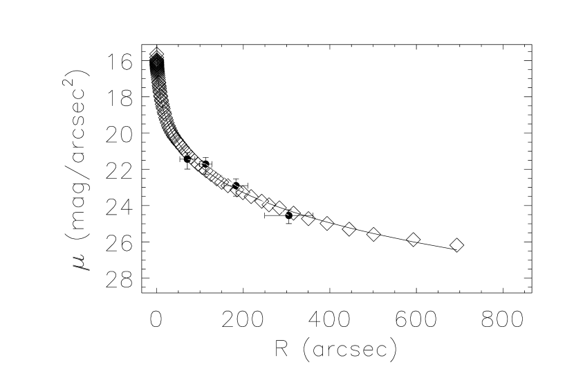
(a)

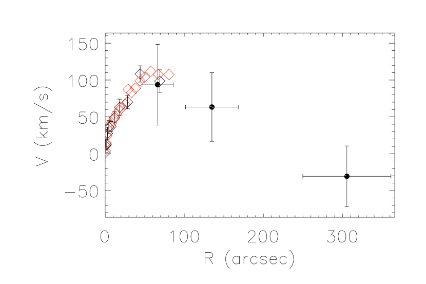
(b)

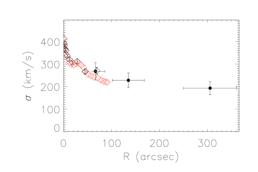
(c)

Figure 3: Comparison of PN data with stellar surface-brightness and long-slit data, along the major axis: (a) The surface-brightness profile measured from photometry in Kormendy et al. (2009) (black diamonds) and the scaled number density calculated from PNe in Teodorescu et al. (2011) (black circles), along with Poissonian errors. (b) and (c) show mean velocity and velocity dispersion profiles respectively, measured from long slits in Pinkney et al. (2003) (black diamonds), adapted from long-slit kinematic data in De Bruyne et al. (2001) (red diamonds, not fitted in the NMAGIC models), and from PNe (black circles).

3 CONSTRAINTS ON THE DISTRIBUTION OF STELLAR VELOCITIES

As kinematic constraints, we combine long-slit kinematics probing the central region and planetary nebula (PN) LOS velocities that probe the outer regions of NGC 4649. Figure 2 illustrates the spatial coverage of the kinematic data. We assume that the $x$-axis increases along East and that the $y$-axis increases along North, and then we rotate the coordinate system to align the $x$-axis with the major axis and the $y$-axis with the minor axis.

3.1 Long-slit kinematics

We use the long-slit absorption-line kinematics of Pinkney et al. (2003), obtained from STIS/HST measurements and ground-based spectroscopic measurements on the 2.4m MDM telescope. They were measured along position angles of 105^∘ (the major axis), 127^∘, 133^∘ and 173^∘ measured from North towards East in the sky, and extending to 69”, 28”, 44”, and 44” respectively. The location and orientation of these slits are shown in Figure 2. Pinkney et al. (2003) derive profiles of the line-of-sight (LOS) mean velocity, velocity dispersion and the higher-order Gauss-Hermite moments $h_{3}$ and $h_{4}$. Figures 3(b) and (c) show the mean velocity and velocity dispersion profiles measured by the long-slit data along the major axis. The mean velocity increases from zero at the centre to about 110 km/s at $\sim 45^{\prime\prime}$ and then decreases to about 95 km/s at $\sim 70^{\prime\prime}$. The velocity dispersion decreases from about 410 km/s at the centre to about 270 km/s at $\sim 70^{\prime\prime}$. For comparison we have overplotted major-axis long-slit kinematic data from De Bruyne et al. (2001), averaged over both sides of the galaxy. The agreement is very good. The data from De Bruyne et al. (2001) are not used in the NMAGIC modelling.

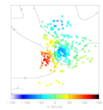
(a)

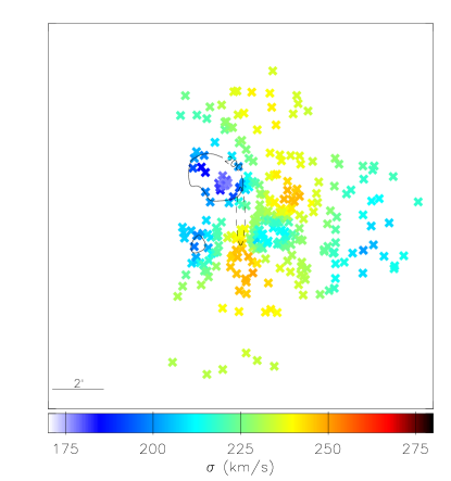
(b)

Figure 4: Smoothed PN kinematic maps: (a) Mean velocity (b) velocity dispersion. The maps are orientated as Figure 2, and therefore the major axis extends from left to right.

3.2 Planetary nebulae

To enable us to probe the mass and orbital structure in the halo of NGC 4649, we use LOS velocities derived from observations of PNe with FORS2 on the VLT and FOCAS on Subaru. The observations and calculations of the velocities are described in a companion paper (Teodorescu et al., 2011). Contaminants from the neighbouring spiral, NGC 4647, are removed using the technique developed by McNeil et al. (2010). This results in a catalogue of 298 PNe extending from 27” to 416”, therefore overlapping with the long-slit kinematic data.

The location of the PNe are shown in Figure 2 and Figure 3(a) compares the measured major-axis $V$-band surface brightness profile with the scaled number density profile of the PNe. The PN number density profile is calculated in a cone of angular width $30^{\circ}$ centred on the major axis, and then scaled to match the photometry. We do not consider incompleteness corrections, which are especially important in the central region, where the bright stellar component masks PNe (e.g. Coccato et al., 2009). However, the PNe number density and surface-brightness profiles agree well, even at the innermost point.

Figure 3(b) shows the mean velocity profile of the PNe calculated in a 30^∘-cone centred on the major axis. In the region of overlap with the long-slit kinematics, the mean velocity profiles agree and further out the PN mean velocity profile decreases outwards to about -20 km/s at $\sim 310^{\prime\prime}$. The large errors bars associated with the PN mean velocity profile allow for a much shallower decrease in the outer parts, consistent with zero at 310”. The combined long-slit and PN major-axis profile shows that the rotation of the stars increases to about 100 km/s at 50” and then starts decreasing outwards.

Figure 3(c) shows the velocity dispersion profile of the PNe calculated in a 30^∘-cone centred on the major axis. The profile agrees with the long-slit kinematic profiles in the region of overlap and then continues to fall less steeply to a value of about 200 km/s at $\sim 310$”. The consistent stellar and PN density and kinematic profiles imply that PNe are good tracers of the stars both in density and kinematics.

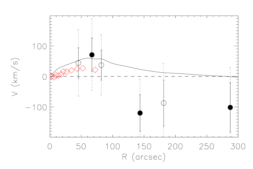
Figure 5: Minor-axis mean velocity profile: The filled, black circles show the mean velocity profile derived from PNe along a 30^∘-cone centred on the minor axis. The open, black circles show the mean velocity profile derived from PNe along a pseudo slit of width 60” centred on the minor axis. The solid black bars denote the 1-$\sigma$ errors and the dotted black bars denote the 2-$\sigma$ errors, estimated from generating pseudo data sets. The solid black line shows the mean velocity profile extracted along the minor axis of the smoothed mean velocity field derived from the PNe. Red diamonds show long-slit kinematic data adapted from De Bruyne et al. (2001).

Figures 4(a) and (b) show smoothed mean velocity and velocity dispersion maps for the region of NGC 4649 covered by the PNe, created by the PNpack suite of IDL routines from Coccato et al. (2009). Rotation approximately about the minor axis is seen clearly in (a). There is also a group of PNe in the top of the field that suggest some rotation about the major axis, a signature of triaxiality. To investigate the strength of this signature, we first extract mean velocity profiles for the PNe along a pseudo slit of width 60” and a cone of angular width 30^∘, centred on the minor axis. Then to estimate the errors on these profiles, we generate 100 pseudo sets of PN LOS velocities at the same positions as the original data, assuming that the line-of-sight velocity distribution (LOSVD) at each point in space is given by the mean velocity and velocity dispersion of the smoothed kinematic fields. For each of the pseudo data sets, we extract new mean velocity profiles as done for the original data set. 1-$\sigma$ and 2-$\sigma$ errors are estimated from the spread in the mean velocity values at each position. Figure 5 shows the resulting minor-axis mean velocity profiles along with the errors. We also extract a mean velocity profile along the minor axis from the smoothed mean velocity field. The profile along the pseudo slit is almost consistent with zero within 1-$\sigma$ errors and both the pseudo-slit and cone profiles are consistent with zero within 2-$\sigma$ errors. The profile derived from the smoothed mean-velocity map is very similar within $\sim 90$” but then decreases to zero, therefore suggesting a lower magnitude of velocity compared to the other two profiles. This profile should however be treated with caution in the outer parts as it is based on far fewer PNe there. The long-slit kinematics of De Bruyne et al. (2001) also show some rotation along the minor axis at about 20 km/s between 50–80”. We do not plot their last point of $\sim 90$ km/s at the last radius of $\sim 95^{\prime\prime}$, as it appears unphysically higher than the rest of the profile. It would however still be in agreement with the PN minor-axis mean velocity profiles and is much less than the measured velocity dispersion. Therefore there is some evidence for triaxiality but it is weak, making it difficult to constrain the viewing angles of the system. Therefore we will proceed with models assuming an oblate, axisymmetric stellar distribution.

4 DYNAMICAL MODELS

Here we describe how we set up the initial model and how we prepare the photometric and kinematic target observables for creating dynamical models with NMAGIC. We then describe how we obtain models first fitting to the light and long-slit constraints, and then models fitting light, long-slit and planetary nebula (PN) constraints.

4.1 NMAGIC

NMAGIC is an N-body made-to-measure code described in de Lorenzi et al. (2007) that has been successfully applied to the intermediate-luminosity elliptical galaxies NGC 4697 (de Lorenzi et al., 2008) and NGC 3379 (de Lorenzi et al., 2009). It finds the best intrinsic distribution of stars and their velocities that projects to fit the photometric and kinematic data. The code builds on the particle-based made-to-measure method of Syer & Tremaine (1996) by accounting for observational errors and therefore allowing for an assessment of the quality of the model fits to the target data. There have also been recent implementations of this method by Dehnen (2009) and Long & Mao (2010).

NMAGIC starts with some initial particle model, where each particle has 3-D spatial coordinates, 3-D velocity coordinates and a weight. The particles are advanced according to the gravitational force to sample their orbits and the weights of the particles are adjusted simultaneously according to the force-of-change (FOC) equation, given in Equation (10) of de Lorenzi et al. (2007) and Equation (22) of de Lorenzi et al. (2008). This equation maximises the merit function, $F$ defined as:

$$F=\mu S-\frac{1}{2}\chi^{2}+\mathcal{L}$$ (2)

where $S$ is a profit function, $\chi^{2}$ measures the goodness of fit to the density and long-slit target observables, and $\mathcal{L}$ is a likelihood term measuring the goodness of fit to the PN target observables. The parameter $\mu$ changes the balance between the profit function and the goodness-of-fit terms. For the profit function, the entropy of the weights is used:

$$S=-\sum_{i}w_{i}\ln\left(\frac{w_{i}}{\hat{w_{i}}}\right)$$ (3)

where $\hat{w_{i}}$ are the initial or prior weights of the particles, and $w_{i}$ are the current weights of the particles. The entropy term causes particle weights to remain close to their priors. Therefore a higher value of $\mu$ will generally result in smoother intrinsic distributions. We have chosen a value of $2\times 10^{3}$, based on previous work using NMAGIC (de Lorenzi et al., 2008, 2009).

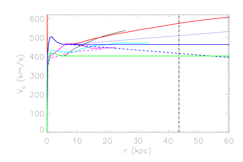
Figure 6: Circular velocity curves of NGC 4649: The solid black line ($VC1$) shows the best-fit circular velocity curve from Das et al. (2010). The solid red line ($VC2$) shows the best-fit circular velocity curve from Shen & Gebhardt (2010). The blue lines show the circular velocity curves based on that from Shen & Gebhardt (2010) but with the outer slope reduced to 0.106 ($VC3$, dotted), 0.000 ($VC4$, solid) and $-0.106$ ($VC5$, dashed). The green line shows the circular velocity curve based on that from Das et al. (2010) but with the outer slope reduced to 0.000 ($VC6$). The vertical black dash-dotted line shows the maximum radial extent of the kinematic constraints. For comparison, the circular velocity curves obtained by Humphrey et al. (2006) (solid, pink), Humphrey et al. (2008) (dashed, pink), and Nagino & Matsushita (2009) (cyan) are overplotted.

4.1.1 The gravitational force

In this work we treat the whole gravitational force as an external force acting on the system, and therefore it can take any form. In the first instance we consider the circular velocity curves derived for NGC 4649 by Das et al. (2010) ($VC1$) using X-ray observations and Shen & Gebhardt (2010) ($VC2$) using optical observations and dynamical models. These two mass distributions only differ in the central $\sim 12$ kpc and are shown in Figure 6. The X-ray observations give information on the temperature and density profiles of the hot gas in massive elliptical galaxies. If the hot gas is approximately spherical and in hydrostatic equilibrium, then the temperature and density profiles are related to the circular velocity curve by:

$$V_{c}^{2}=-\frac{k_{b}T}{\mu m_{p}}\frac{\textrm{d}\ln P}{\textrm{d}\ln r}$$ (4)

where $T$ is the temperature of the gas and $r$ is the 3-D radius from the centre of the galaxy. $\mu=0.61$ is the average gas particle mass in terms of the proton mass, $m_{p}$. This value of $\mu$ corresponds to a helium number density of $7.92\times 10^{-2}$ and 0.5 solar abundance of heavier elements. We assume that the gas is ideal and therefore the gas pressure $P=nk_{B}T$, where $n$ is the particle number density of the gas. Das et al. (2010) applied hydrostatic equilibrium using a new non-parametric Bayesian approach to density and temperature profiles of the hot gas derived from Chandra and XMM-Newton observations (Churazov et al., 2010).

The best-fit mass profile of Shen & Gebhardt (2010) was obtained from axisymmetric Schwarzschild models assuming a stellar density profile from Kormendy et al. (2009) and fitting to long-slit kinematic constraints from Pinkney et al. (2003) and GC LOS velocities from Hwang et al. (2008).

In both cases we assume that the gravitational force is spherically symmetric. Therefore as the stars are assumed to have an oblate, axisymmetric distribution, the dark matter halo must be prolate in the centre where the stars dominate, and almost spherical in the outer parts where the dark matter dominates.

4.1.2 The initial particle model

We set up an initial model of 750000 particles extending to $\sim 205$ kpc. We assume a density distribution of the particles given by a spherical deprojection of the circularly-averaged surface-brightness profile. We define the intrinsic stellar velocity distribution using the circularity functions of Gerhard (1991), resulting in an anisotropy profile ($\beta=1-\sigma_{\theta}^{2}/\sigma_{r}^{2}$) that is isotropic in the centre but moderately radial ($\beta\sim 0.5$) in the outer parts. This choice reflects the results of numerical simulations by Abadi et al. (2006) and Oñorbe et al. (2007). We then solve for the energy part of the distribution function assuming a potential given by $VC1$. The particles’ coordinates and velocities are chosen according to the complete distribution function after Debattista & Sellwood (2000) and they are assigned equal weights of $w_{i}=1/750000$ to produce the initial particle model. As the gravitational field is fixed with time in our models, the orbits of the particles do not change with time. Therefore our initial particle model is conceptually very similar to the orbit libraries used as initial conditions in Schwarzschild models.

4.1.3 Preparation of stellar density target observables

We represent the 3-D luminosity density profiles obtained for each inclination from the deprojection in terms of $A_{lm}$ coefficients (de Lorenzi et al., 2007) between 0.3 kpc and 201 kpc. 0.3 kpc is the innermost radius of the X-ray circular velocity curve ($VC1$) and 201 kpc is the radius at which the density of the initial particle model starts falling off from the deprojected density profile. As the stellar distribution is assumed to be axisymmetric we set all moments that describe non-axisymmetry to zero. We calculate the $A_{lm}$s over a grid of 60 radii. Poissonian errors are assumed for the radial mass profile and Monte-Carlo simulations are used to determine errors for the higher-order mass moments.

$i$ (∘)	$\chi^{2}_{\textrm{alms}}$	$\chi^{2}_{\textrm{long-slit}}$	$\chi^{2}$	$-F$
(1)	(2)	(3)	(4)	(5)
45	0.468, 0.260	0.632, 0.521	0.534, 0.366	1374.3,1108.0
60	0.179, 0.210	0.537, 0.469	0.324, 0.315	746.4,713.0,
75	0.141, 0.187	0.542, 0.477	0.304, 0.304	644.6,641.6
90	0.220, 0.196	0.655, 0.518	0.396, 0.326	761.5,661.5

Table 1: Best-fit NMAGIC models for NGC 4649 assuming different inclinations in the X-ray ($VC1$, left in columns (2)–(5)) and dynamical ($VC2$, right in columns (2)–(5)) potentials : (1) Inclination assumed for model, (2) $\chi^{2}$ per $A_{lm}$ target observable, (3) $\chi^{2}$ per long-slit target observable, (4) $\chi^{2}$ per target observable, and (5) the merit function. There are 960 density target observables and 655 long-slit target observables.

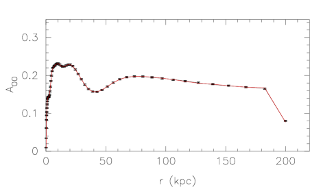
Figure 7: Fit to the first moment of the $A_{lm}$s or differential stellar mass distribution for an inclination of 75^∘ in the circular velocity curves $VC1$ (black) and $VC2$ (red).

4.1.4 Preparation of kinematic target observables

As we are assuming that the stellar distribution in NGC 4649 is an oblate, axisymmetric system rotating about its minor axis, for every mass element at $(x,y,v)$, we can assume that there is also a mass element at $(-x,-y,-v)$ and a mass element at $(-x,y,-v)$. Therefore we can add three more long slits at position angles of $105^{\circ}-68^{\circ}=37^{\circ}$, $105^{\circ}-28^{\circ}=77^{\circ}$ and $105^{\circ}-22^{\circ}=83^{\circ}$, which are spatial reflections around the $x$-axis of the long slits positioned at 173^∘, 133^∘ and 127^∘. The PNe are increased 4-fold by imposing the above reflections, resulting in a sample of 1192 PNe. As NMAGIC is a particle-based code, the weight of each particle will be changed more evenly over each orbit with the 4-fold sample compared to the unfolded sample.

For NMAGIC the light in each of the slit cells needs to be calculated, as the light-weighted kinematics are fit rather than the kinematics directly. The light in the cells is calculated by integrating the surface-brightness distribution over the dimensions of each of the slit cells (assumed to have a width of 5”) using a Monte-Carlo integration scheme.

To fit the PN LOS velocities, we use the likelihood method used in de Lorenzi et al. (2008, 2009). In this method the particles are binned in radial and angular segments to calculate the LOSVD in each segment. Then the likelihood of each PN belonging to the LOSVD of its segment is maximised for all the PNe. For the binning, we choose 3 radial bins (corrected for an average projected ellipticity of 0.857) and 6 equally-spaced angular bins with the first centred on the major axis.

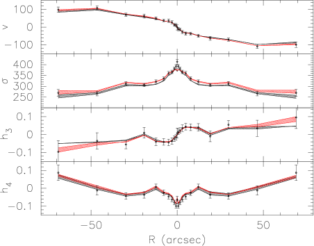
(a)

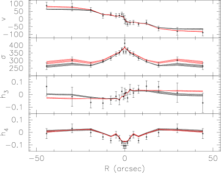
(b)

Figure 8: Fits to the long-slit data (a) along the major axis and (b) along a slit placed at a position angle of 133^∘: From the top down are shown mean velocity, velocity dispersion and the Gauss-Hermite moments $h_{3}$ and $h_{4}$. Black circles show the data, the black region shows the models for the various inclinations probed in $VC1$, and the red region shows the models probed for the various inclinations in $VC2$.

4.1.5 Logistics of a ‘run’

For each run we fit the desired data starting with the initial particle model generated above. There is an initial relaxation phase of 2000 steps where the particles are advanced according to the force and their weights are not changed. Each step is equivalent to $4.4\times 10^{5}$ yrs. We then have another 2000 steps during which we temporally smooth the observables and the weights of the particles are still not changed. Then the core phase of the run starts, where the particles are advanced according to the gravitational force and the weights of the particles are changed according to the FOC equation. Once the fractional change in the total $\chi^{2}$ falls to less than 1.5$\times 10^{-3}$ over 5000 steps, we define the model to have converged. Finally this is followed by a free evolution, where the particles are advanced for a further 20000 steps and the weights are no longer changed, to check that the converged model has been sufficiently phase-mixed. The particles are advanced using an adaptive leapfrog scheme.

In the FOC equation, the respective contributions of the $A_{lm}$, long-slit kinematic and PN kinematic terms can be very different. The errors are very small for the $A_{lm}$s but much larger for the PNe, resulting in a much larger contribution from the $A_{lm}$ terms to the FOC equation. As a result, changes made to the weights of the particles by the PN data will be small, and need to be made many times before a converged model is reached. Therefore as the PNe and to some extent the long-slit are important in the halo, after some tests, we increase their contributions to the FOC equation by factors of 20 and 2 respectively, to ensure that the halo is adequately modelled.

4.2 Models fitting density and long-slit kinematic constraints only

First we would like to understand whether the observational constraints are able to differentiate between the dynamical mass model of Shen & Gebhardt (2010) ($VC2$) and the X-ray mass profiles in the literature, which are lower in the central $\sim 12$ kpc. For the X-ray mass profile, we choose that of Das et al. (2010) ($VC1$), which is very similar to that of Shen & Gebhardt (2010) in the outer parts. As the potentials only differ in the central 12 kpc, and the PN kinematic constraints are much weaker than the density and long-slit kinematic constraints, we will not include the PNe for these models. This saves considerable computational time because the PNe are further out and therefore the particles need to be integrated for longer there to achieve convergence. Additionally the likelihood method is itself computationally expensive.

We carry out NMAGIC models assuming inclinations of 45^∘, 60^∘, 75^∘ and 90^∘ for the stellar distribution, for which we also carried out the deprojections of the photometry. Table 1 shows the $\chi^{2}$ per data point for the density observables, the long-slit kinematics, all the observables, and the merit function $F$ of the final models in each inclination and potential. NMAGIC fits to the light-weighted kinematic observables as well as the light in each cell, and therefore the long-slit $\chi^{2}$ is calculated as a sum over these variables.

We find that both potentials prefer (in the sense of a lower $\chi^{2}$) an inclination of $75^{\circ}$ of the stellar system. In this inclination, neither potential is preferred by the combination of the photometric and long-slit constraints.

4.2.1 Fits to the observables

Figure 7 shows the fits in both potentials to the first moment of the $A_{lm}$s or differential stellar mass distribution for the most favoured inclination of 75^∘, in potentials $VC1$ and $VC2$. The fits are almost indistinguishable from each other, and match the density constraints very well. Figure 8 shows the fits to the $v$, $\sigma$, $h_{3}$ and $h_{4}$ moments along the major-axis slit and the slit placed along 133^∘, for both potentials and all inclinations. In general the fits are very similar but there are some systematic differences. The models in $VC1$ produce mean velocity profiles with a lower magnitude ($\sim 5$–20 km/s), a lower velocity dispersion ($\sim 10$–30 km/s), an $h_{3}$ moment with a lower magnitude (0.01–0.02) and an $h_{4}$ moment that is very marginally lower on average. These differences are generally a small fraction of the error bars.

All the models find a $\chi^{2}$ per data point less than 1. Then if the number of degrees of freedom is approximately equal to the number of data points, then we can be satisfied that we are fitting the data well, and even over-fitting. In reality however, the number of degrees of freedom is difficult to estimate because it is equal to the number of constraints subtracted by the number of parameters. The number of parameters is equal to the number of model parameters (e.g. halo, $M/L$, inclination) plus the number of weights that we are fitting, which is the number of particles. The number of constraints is equal to the number of data points plus the number of constraints introduced by the profit function, which is difficult to quantify.

We now attempt a $\Delta\chi^{2}$ analysis as done for example in Shen & Gebhardt (2010). If we say each of our models could be characterised by four parameters (inclination, mass-to-light ratio and two parameters for the dark matter halo) that need to be determined, then $\Delta\chi^{2}$ for a 68.3% confidence interval is 4.7 (Press et al., 1986), or 0.003 per data point for 1615 observables (960 $A_{lm}$ and 655 long-slit target observables). Therefore in the absence of systematic errors, any models with a $\chi^{2}$ of more than 0.003 per data point greater than the minimum $\chi^{2}$ per data point can be ruled out because we know they must definitely be outside the 68.3% confidence range around the true best model. Table 1 shows that the density observables most prefer an inclination of 75^∘ but the long-slit observables most prefer an inclination of 60^∘, in both potentials. Considering the data altogether, both potentials prefer an inclination of 75^∘. Generally the dynamical potential is preferred over the X-ray potential except for in the most favoured inclination, where $VC1$ and $VC2$ are equally preferred. As the remaining models achieve a $\chi^{2}$ of more than 0.003 per data point away from the minimum $\chi^{2}$ of 0.304 per data point, we would rule them out with 68.3% confidence using the $\Delta\chi^{2}$ approach.

Potential	Slit PA (∘)	$v$	$\sigma$	$h_{3}$	$h_{4}$
X-ray	105	0.131	-0.196	-0.013	0.032
($VC1$)	127	-0.005	-0.048	-0.036	-0.179
	133	0.110	-0.015	-0.014	0.165
	173	0.041	-0.170	0.033	-0.003
	All	0.073	-0.111	-0.007	0.009
Dynamical	105	0.041	0.113	-0.012	0.149
($VC2$)	127	-0.043	0.086	-0.013	-0.141
	133	-0.032	0.228	0.018	0.188
	173	0.038	0.128	0.031	0.067
	All	0.019	0.139	0.006	0.073

Table 2: Systematic differences between model and observed $v$, $\sigma$, $h_{3}$ and $h_{4}$, averaged over each of the first four slits for radii outside 4”, and then averaged over all the slits.

We also quantify the systematic difference, $\Delta S$, between the model and data in both potentials:

$$\Delta S=\frac{1}{n}\sum_{j=1}^{j=n}\frac{K_{M,j}-K_{O,j}}{\epsilon_{K,j}}$$ (5)

where $K$ represents the observable $v$, $\sigma$, $h_{3}$ or $h_{4}$, $M$ is the model value, $O$ is the observed value, $n$ is the number of observables, and $\epsilon_{K,j}$ is the error on the observed value. $\Delta S$ is calculated for each moment averaged over each of the first four slits (the remaining three slits are only reflections of the first three) for radii outside 4”, and then averaged over all the slits. Only the results in the most favoured inclination of 75^∘ are shown in Table 2. In $VC1$, the magnitude of the model mean velocity is a little higher, while the velocity dispersion is systematically a little lower than the observations. The systematic differences in the $h_{3}$ and $h_{4}$ moments are smaller. In $VC2$, the systematic differences are biggest also in the velocity dispersion, which is higher than the observations on average, and in the $h_{4}$, which are also systematically higher. Systematic differences between the model and the data seem similar in both potentials and are also comparable to deviations used to rule out models ($\sqrt{\Delta\chi^{2}=0.003}=0.055$ per data point). This implies that neither mass model is exactly correct and that the true mass distribution lies somewhere in between, or that systematic effects (e.g. triaxiality) play a role. Therefore the $\Delta\chi^{2}$ approach should be used with caution.

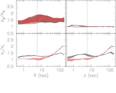
Figure 9: Intrinsic kinematics: The left set of panels show the ratio of the radial velocity dispersion to the tangential velocity dispersion (bottom), and the ratio of the azimuthal velocity dispersion to the meridional velocity dispersion (top), along $R$. The right set of panels show the same along $z$. The black region corresponds to the models carried out for various inclinations in $VC1$ and the red region corresponds to the models carried out for various inclinations in $VC2$, fitting photometric and long-slit constraints only. The dashed black line shows the radial extent of the kinematic constraints.

4.2.2 The orbital structure

As we have assumed an oblate, axisymmetric system, we can average the intrinsic kinematics over the azimuthal angle, $\phi$. This reduces the spatial coordinates to $R$ in the equatorial plane, which is the major axis of the system, and $z$ in the meridional plane, the minor axis of the system. Figure 9 shows the ratio of radial to tangential velocity dispersions ($\sigma_{r}/\sigma_{t}$), and the ratio of azimuthal to meridional velocity dispersions ($\sigma_{\phi}/\sigma_{\theta}$) along $R$ and $z$. The tangential velocity dispersion is defined as $\sigma_{t}=\sqrt{(\sigma_{\theta}^{2}+\sigma_{\phi}^{2})/2}$. Within the radial extent of the kinematic constraints, there is a bias towards radial orbits in $VC1$ along $R$ and $z$ with $(\sigma_{r}/\sigma_{t})_{max}\sim 1.5$. In the same region the orbital structure in $VC2$ is almost isotropic along $R$ and $z$. On average the ratio of the radial to tangential velocity dispersions is 1.2–1.3 higher in $VC1$ than in $VC2$ throughout. The two components of tangential velocity dispersions have similar contributions in both potentials along $z$, and in the equatorial plane the azimuthal dispersions dominate. In both potentials, variation with inclination is greatest in the ratio between the azimuthal and meridional dispersions along $R$.

$V_{c}$	$\chi^{2}_{\textrm{alms}}$	$\chi^{2}_{\textrm{long-slit}}$	$\chi^{2}$	$-LH$	$-F$
(1)	(2)	(3)	(4)	(5)	(6)
$VC2$	0.268	0.510	0.366	3107.0	4232.3
$VC3$	0.201	0.496	0.321	3097.1	4087.1
$VC4$	0.196	0.489	0.315	3087.0	3988.7
$VC5$	0.236	0.480	0.335	3079.7	4006.0
$VC6$	0.213	0.818	0.458	3067.2	4091.3

Table 3: Best-fit NMAGIC models for NGC 4649 for an inclination of 75^∘ in a range of circular velocity curves: (1) Circular velocity curve, (2) $\chi^{2}$ per $A_{lm}$ target observable, (3) $\chi^{2}$ per long-slit target observable, (4) $\chi^{2}$ per target observable, (5) log-likelihood of PNe belonging to particle LOSVDs, and (6) the merit function.

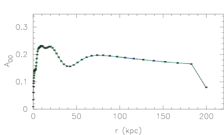
Figure 10: Fit to the first moment of the $A_{lm}$s or differential stellar mass distribution for an inclination of 75^∘ in potentials $VC2$ (solid, red), $VC3$ (dotted, blue), $VC4$ (solid, blue), $VC5$ (dashed, blue), and $VC6$ (green).

4.3 Models fitting density, long-slit kinematic constraints and planetary nebula line-of-sight velocities

Now we will carry out models including also the PN kinematics, so that we can check whether the PN kinematics are consistent with the halo in the mass determinations of Das et al. (2010) and Shen & Gebhardt (2010). As both potentials have almost the same halo we first carry out a model in the potential of Shen & Gebhardt (2010) ($VC2$). We find that the model velocity dispersions are systematically too high and therefore repeat models in a range of potentials with less massive haloes (see Figure 6 and Table 3). Incorporating the PNe, the models prefer a halo with a significantly lower circular velocity of $\sim 463$ km/s compared to a value of 570 km/s at 45 kpc found in Shen & Gebhardt (2010).

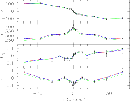
Figure 11: Fits to the long-slit data: From the top down are shown mean velocity, velocity dispersion and the Gauss-Hermite moments $h_{3}$ and $h_{4}$ for an inclination of 75^∘ and for the slit placed along the major axis. Black circles show the data and the lines show fits in potentials $VC2$ (solid, red), $VC3$ (dotted, blue), $VC4$ (solid, blue), $VC5$ (dashed, blue), and $VC6$ (green).

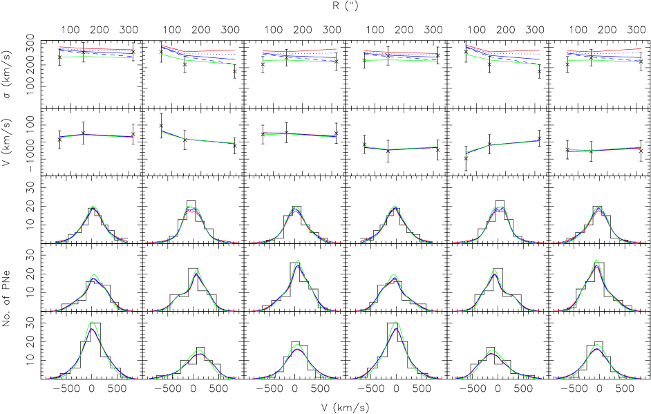
Figure 12: Fits to the PN data for an inclination of 75^∘. Each of the plots in the bottom three rows shows the LOSVD in segments. Going upwards are segments at radii of 64”, 145” and 316” and going towards the right are angular segments centred on 0^∘ (major axis), 60^∘, 120^∘, 180^∘, 240^∘, and 300^∘. The kinematics along the latter three segments are reflections of the kinematics along the first three segments because of the oblate, axisymmetry imposed on the observational constraints. The top two sets of panels show the mean velocity and velocity dispersion profiles along the angular segments. The fits are in potentials $VC2$ (solid, red), $VC3$ (dotted, blue), $VC4$ (solid, blue), $VC5$ (dashed, blue), and $VC6$ (green).

4.3.1 Fits to the observables

Figures 10, 11 and 12 show the fits to the first moment of the $A_{lm}$s, the fits to the Gauss-Hermite moments along the major axis and the fits to the PN LOS velocities, in $VC2$, for an inclination of 75^∘. Table 3 shows the statistics of the fits obtained for the new model incorporating the PN data. Even though visually the fits look very much the same in the $A_{lm}$s and long-slit, the $\chi^{2}$ values for the fit to the $A_{lm}$s and long-slit are slightly higher than before, though still much less than 1. This shows that in this potential, by trying to fit the PNe, the fits to the $A_{lm}$s and long-slit are slightly compromised. Looking at the PN kinematics, it appears that the mean velocity profiles are fit well but the velocity dispersions of the model are systematically higher than that measured by the PNe. This implies that the PNe are not consistent with the outer part of $VC2$, and therefore also $VC1$ (both potentials agree very well outside $\sim 12$ kpc).

4.3.2 Fits in less massive haloes

As the PN dispersions are systematically lower than predicted by the models, we also investigate additional circular velocity curves with less massive haloes (Figure 6). We fit a straight line to $VC2$ outside 7.6 kpc and obtain a slope of 0.212. We create three additional curves where the outer slopes are 0.106 ($VC3$), 0.0 ($VC4$) and -0.106 ($VC5$). Finally we consider a curve that follows $VC1$ until 4.9 kpc and then also has an outer slope of 0.0 ($VC6$). The model fits in these potentials are overplotted on Figures 10, 11, 12 and the statistics of the fits are given in Table 3. The $\chi^{2}$ values show that the $A_{lm}$s and long-slit data most prefer $VC4$, and the likelihood values show that the PNe most prefer $VC6$. The merit function $F$ is a combination of the $\chi^{2}$ values, likelihood and entropy, and this is a maximum in the potential $VC4$. Therefore we consider this the best of the potentials tried. The differences between the models in the $A_{lm}$s and fits to the long-slit kinematics are small except in $\sigma$ and $h_{4}$, which are systematically lower in $VC6$ compared to potentials $VC2$–$VC5$. Figure 12 shows that the PN velocity dispersions are however very sensitive to the mass in the halo.

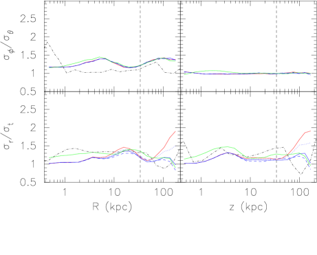
Figure 13: Intrinsic kinematics: The left set of panels show the ratio of the radial velocity dispersion to the tangential velocity dispersion (bottom), and the ratio of the azimuthal velocity dispersion to the meridional velocity dispersion (top), along $R$. The right set of panels show the same along $z$. The dash-dotted black line shows the results of Shen & Gebhardt (2010) who fit GC kinematics instead of PN kinematics. The fits are done in potentials $VC2$ (solid, red), $VC3$ (dotted, blue), $VC4$ (solid, blue), $VC5$ (dashed, blue), and $VC6$ (green). The dashed black line shows the radial extent of the kinematic constraints.

4.3.3 The orbital structure

Figure 13 shows that within $\sim 6$ kpc the intrinsic velocity dispersions are isotropic to mildly radial along $R$ and $z$ in potentials $VC2$–$VC5$ and moderately radial in $VC6$, consistent with the findings in Section 4.2.2. Further out until the radial extent of the PN kinematic constraints, the orbital structure in all potentials becomes moderately radial along $R$ and more isotropic along $z$. The two components of tangential velocity dispersions have similar contributions in all the potentials, and in the equatorial plane the azimuthal dispersions dominate over meridional velocity dispersions.

5 DISCUSSION

Here we discuss what we have learned about the dark matter halo, orbital structure and inclination of the stellar system in NGC 4649. We also discuss whether the PNe and GC systems are dynamically consistent with each other, and whether the X-ray mass distributions can be used to determine dark matter mass fractions and orbital structures in massive elliptical galaxies.

5.1 The dark matter halo of NGC 4649

Figure 6 shows the circular velocity curves that we have probed in this work, compared to other recent determinations from Chandra observations (Humphrey et al., 2006; Humphrey et al., 2008) and a combination of Chandra and XMM-Newton observations (Nagino & Matsushita, 2009).

Our models fitting only density and long-slit kinematic constraints cannot distinguish between the circular velocity curves of Das et al. (2010) and Shen & Gebhardt (2010), which differ only in the central $\sim$ 12 kpc. A look at the systematic differences between the models and observations in these potentials suggests that the true circular velocity curve in the central $\sim 12$ kpc probably lies somewhere between 425–500 km/s.

Models created incorporating additionally PN kinematics (Teodorescu et al., 2011) prefer a circular velocity curve that is flat outside $\sim 12$ kpc at a value of $\sim 463$ km/s. This is most consistent with the X-ray determination of Nagino & Matsushita (2009), slightly higher than the determinations of Humphrey et al. (2006); Humphrey et al. (2008), and lower than the determinations of Das et al. (2010) and Shen & Gebhardt (2010). The sensitivity of the PN velocity dispersions to the circular velocity curve in the halo may be a result of a light density profile that falls off approximately as -3 and an almost flat circular velocity curve. Gerhard (1993) showed that for such systems, the projected velocity dispersions are constant and independent of anisotropy. The constant circular velocity $V_{c}$ is then related to the constant projected velocity dispersion $\sigma_{P}$ by $V_{c}=\sqrt{3}\times\sigma_{P}$. The average velocity dispersion of the PNe outside $\sim 70$” is $\sim 240$ km/s, therefore predicting a circular velocity in the halo of 416 km/s. This lies in between the value of 383 km/s of $VC6$, the halo most preferred by just the PNe, and the value of 463 km/s of $VC4$, the halo most preferred considering all the data together.

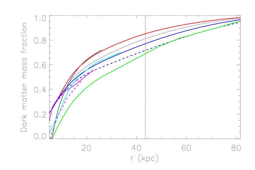
Figure 14: Dark matter mass fraction of NGC 4649 according to potentials $VC1$ (black), $VC2$ (red), $VC3$ (solid, blue), $VC4$ (dotted, blue), $VC5$ (dashed, blue), and $VC6$ (green). For comparison, the dark matter mass fractions calculated from circular velocity curves obtained by Humphrey et al. (2006) (solid, pink), Humphrey et al. (2008) (dashed, pink), and Nagino & Matsushita (2009) (cyan) are also overplotted.

To estimate the dark matter mass fraction, we first calculate the luminosity enclosed within radius $r$ by integrating over the luminosity density profile obtained from the spherical deprojection of the surface-brightness profile. To obtain the mass in stars we multiply this with a constant stellar population mass-to-light ratio estimated in Teodorescu et al. (2011). They used ages and metallicities in Trager et al. (2000) and the evolutionary population synthesis models of Maraston (1998, 2005) for a Salpeter initial mass function with a lower mass limit of $0.1M_{\odot}$. Their value of 10 in the $B$ band corresponds to a value of about 7.6 in the $V$ band. Assuming that the mass in gas is negligible, we subtract the mass in stars from the total mass. Figure 14 shows the dark matter mass fractions corresponding to the potentials we have explored and the potentials from the literature shown in Figure 6. The dark matter mass fraction corresponding to our best potential $VC4$ is $\sim$ 0.39 at 10.5 kpc (1$R_{e}$), 0.5 at about 16 kpc ($1.5R_{e}$) and $\sim 0.78$ at the radius of the last PN ($\sim$45 kpc $\approx$ 4$R_{e}$). Figure 14 shows that our determination is most similar to that of Nagino & Matsushita (2009) as for the circular velocity curve.

There are also several determinations of dark matter fractions for other elliptical galaxies in the literature. Nagino & Matsushita (2009) analysed Chandra and XMM-Newton observations for a sample of 22 elliptical galaxies and found equality between dark matter and luminous matter at around $3R_{e}$ and a dark matter mass fraction of around 0.66 at $\sim 6R_{e}$. Gerhard et al. (2001) and Thomas et al. (2007) found dark matter mass fractions within $1R_{e}$ of 10–40% and 10–50% respectively, for samples of nearby and Coma cluster elliptical galaxies. Gerhard et al. (2001) found equality between the mass contributions of the dark matter and luminous components at 2–4$R_{e}$, and for the Coma galaxies with sufficiently spatially extended data (generally the less luminous ellipticals), Thomas et al. (2007) found dark matter mass fractions between 65–75% at 4$R_{e}$.

Treu & Koopmans (2004) used a combined lensing and stellar dynamical approach to obtain the dark matter mass fractions of elliptical and lenticular galaxies up to a redshift of 1, and found projected values of 0.15–0.65 within a cylinder of radius 1$R_{e}$. For massive early-type galaxies taken from the Sloan Lens ACS Survey (SLACS), Auger et al. (2009) and Auger et al. (2010) found that the dark matter fraction within $R_{e}/2$ ranges between $\sim 0.3$–0.7 assuming a Chabrier stellar IMF (the Salpeter stellar IMF gives lower dark matter mass fractions in their study that are sometimes negative), with more massive galaxies having higher dark matter mass fractions. Grillo (2010) used simple mass models to estimate a dark matter mass fraction of $0.64_{0.11}^{0.08}$ projected inside a cylinder of radius 1$R_{e}$ for a sample of approximately 170000 massive, elliptical galaxies observed in SDSS, from which the SLACS sample is obtained. We estimate the effect of projection on the dark matter mass fraction by assuming an NFW density profile for the dark matter profile, with a virial radius of 300 kpc and a concentration of 10 (typical for elliptical galaxies). The ratio of the dark matter mass within a cylinder of length two virial radii along the LOS and radius $R_{e}$, to that within a sphere of radius $1R_{e}$ is about 2. Assuming that the ratio of the stellar mass between the two regions is almost 1, then the dark matter mass fraction calculated within a sphere of radius $1R_{e}$ would be lower, for example 0.47 instead of 0.64.

Oñorbe et al. (2007) analysed the mass and velocity distributions of elliptical-like objects at zero redshift in a set of self-consistent hydrodynamical simulations set in the current cosmological paradigm. They found that the objects are embedded in massive, dark matter haloes with dark matter mass fractions ranging between 0.3–0.6 at 1$R_{e}$.

To summarise, there is a range in the dark matter mass fractions at 0.5–$1R_{e}$ in the literature, and the value we obtain for NGC 4649 is near the middle of this range. Further out, the dark matter mass fractions obtained by Gerhard et al. (2001), Thomas et al. (2007) and Nagino & Matsushita (2009) suggest on average a more diffuse dark matter halo than the one we find for NGC 4649. This may be because their samples include elliptical galaxies at a range of luminosities, while massive elliptical galaxies like NGC 4649 may have more massive dark matter haloes (e.g. Cappellari et al., 2006; Auger et al., 2010).

5.2 Orbital structure in NGC 4649

The central $\sim 6$ kpc of NGC 4649 has an isotropic ($\beta=1-\sigma_{t}^{2}/\sigma_{r}^{2}\sim 0$) to mildly radial ($\beta\sim 0.4$) orbital structure according to the dynamical potential of Shen & Gebhardt (2010) and the X-ray potential of Das et al. (2010), between which we are unable to distinguish. If we assume that the true mass distribution in the central $\sim 12$ kpc lies somewhere between these two, as suggested by the systematic differences between the models and the observations in the two potentials, then we can infer an orbital structure in this region of $\beta\sim 0.2\pm 0.2$. Using additionally the PN constraints and exploring several potentials, we find that the orbital structure outside $\sim 4$ kpc becomes slightly more radial ($\beta\sim 0.5$) along $R$, but more isotropic along $z$, with little dependence on the exact halo assumed. Along $R$, the azimuthal velocity dispersions are slightly higher than the meridional velocity dispersions throughout, indicating that the stellar system may be flattened by a meridional anisotropy in the velocity dispersion tensor (Dehnen & Gerhard, 1993a, b; Thomas et al., 2009). Thomas et al. (2009) also use axisymmetric toy models to show that flattening by meridional anisotropy maximises the entropy for a given density distribution. Along $z$, the azimuthal and meridional velocity dispersions are equal, as one would expect for an oblate, axisymmetric system.

There is no general consensus on the orbital structure in the outer parts of elliptical galaxies. Dynamical models fitting outer kinematics of intermediate-luminosity elliptical galaxies have found a moderately radial orbital structure in the halo of NGC 4697 (de Lorenzi et al., 2008). In NGC 3379, de Lorenzi et al. (2009) found that systems with both isotropic and moderately radial orbital structures were consistent with the data, and Napolitano et al. (2009) found moderately radial anisotropy in the halo of NGC 4494. Dynamical models fitting outer kinematics in more massive elliptical galaxies such as NGC 1399 (Schuberth et al., 2010, the GCs used are believed to trace the stellar kinematics in this galaxy) and NGC 4374 (Napolitano et al., 2010) have found mildly radial and isotropic orbital structures in the halo respectively. For the elliptical galaxies in the Coma cluster, which have a range of luminosities, Thomas et al. (2007) found mild radial anisotropy along the major axis and sometimes tangential anisotropy along the minor axis.

From simulations, Abadi et al. (2006) found that the outer haloes of massive ellipticals are strongly radial due to smaller galaxies that have been accreted on to the central object. The analysis of Oñorbe et al. (2007) of elliptical-like objects at zero redshift also found a radial orbital structure for the stars at an almost constant value of $\beta\sim 0.5$ throughout. Thomas et al. (2009) analysed the orbital structure of collisionless disc merger remnants from Naab & Burkert (2003) and found them to be strongly radially anisotropic.

To summarise, dynamical models show that the orbital structure in the halo of massive elliptical galaxies is isotropic to quite radial, but less so than expected from simulations. Thomas et al. (2009) arrived at a similar conclusion and suggested that this could be due to gas dissipational effects.

5.3 The inclination of NGC 4649

The surface-brightness and long-slit kinematic constraints in both potentials $VC1$ and $VC2$ prefer an inclination of 75^∘ out of the four inclinations we have probed. As we only explore a coarse grid of inclinations at intervals of $15^{\circ}$, we can attach an error of $7.5^{\circ}$ to our best inclination. Thus it appears that even if the X-ray potential may not be completely correct throughout, it may be used to find an approximate value for the inclination of the system. This appears to be contrary to the work done for example by Krajnović et al. (2005), who found a degeneracy in the determination of the inclination in their construction of axisymmetric models for the elliptical galaxy NGC 2974. However, we have assumed the same spherical total potential in all the inclinations for our first set of models, and only the stellar distribution was axisymmetric and varied according to the inclination. To understand this issue in more depth, a range of mass profiles need to be explored in each inclination to see whether equally good but different mass profiles can be found for each of the inclinations.

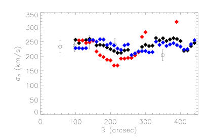
(a)

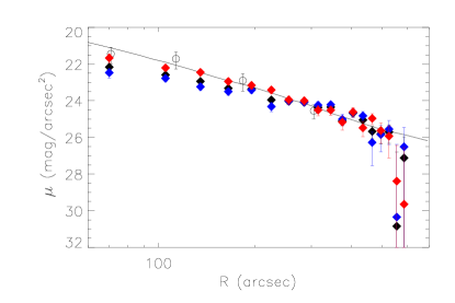
(b)

Figure 15: Properties of the GC populations: (a) Velocity dispersion profiles of all GCs (filled, black diamonds), red GCs (filled, red diamonds) and blue GCs (filled, blue diamonds) compared to that measured by the PNe (open, black circles). The errors on the GC velocity dispersions are approximately twice as big as the errors shown on the PN velocity dispersions. (b) Surface number density profiles of all GCs (filled, black diamonds), red GCs (filled, red diamonds) and blue GCs (filled, blue diamonds) compared to the stellar surface-brightness distribution (solid, black line) and the surface number density of PNe (open, black circles). The GC points are not independent as they are obtained with a moving window average.

5.4 Are the PNe and GCs dynamically consistent with each other?

The NMAGIC models show that the PN kinematics prefer a less massive halo and a less radial orbital structure than that derived from models using the stellar density profile and GC kinematics in Shen & Gebhardt (2010). However if both the PN and GC systems are in equilibrium, the same halo should be preferred although the orbital structure may be different. To obtain a deeper insight into this discrepancy, we examine the photometric and kinematic constraints assumed for the PNe and GCs in more detail. Figure 15(a) compares the velocity dispersion profile calculated in circular rings from the PNe to those for red, blue, and all GCs calculated by Hwang et al. (2008). The errors bars on the GC kinematics are not shown because they mask all the other points but are approximately twice as big as the errors shown on the PN velocity dispersions. One can see that between 100” and 200”, the PN velocity dispersions appear to be in agreement with the dispersions measured by the blue GCs (and therefore the total sample because the blue GCs dominate in numbers). The velocity dispersion of the red GCs decreases to almost 150 km/s at $\sim$210” and then increases dramatically to about 320 km/s at $\sim$390”. The last PN velocity dispersion point at $\sim$350” calculated in a ring extending from 260–440” has a value of $203\pm 19$ km/s. Averaging all the GCs velocity dispersions in this region gives $\sim 240\pm 22$ km/s for 61 GCs, which would correspond to the values fit by Shen & Gebhardt (2010). This is only just consistent and therefore it is possible that the PNe and GCs trace different kinematics.

Figure 15(b) compares the surface-brightness distribution of the stars with scaled surface number densities calculated from PNe in Teodorescu et al. (2011) and GCs from Hwang et al. (2008). Between 200–450”, the surface densities of the whole GC population follows the stellar surface-brightness distribution well. Further in, the GC density profile is shallower than that of the stars and outside this region the density profile falls off more steeply than the stars, though the associated errors are larger. Therefore the density profile of the GCs appears to be different from that of the stars.

The GCs could still be in equilibrium however but just form a separate dynamical system in the same potential. This can be quantified using the spherical second-order Jeans equation, relating the second-order moments of the intrinsic velocity distribution to the density profile of the stars, and the potential in which they move (Binney & Tremaine, 1987):

$$\frac{\textrm{d}}{\textrm{d}r}(\nu(r)\sigma_{r}^{2}(r))+\frac{2\beta(r)}{r}\nu(r)\sigma_{r}^{2}(r)+\nu(r)\frac{V_{c}^{2}}{r}=0$$ (6)

where $V_{c}$ is the circular velocity curve, $\sigma_{r}$ is the intrinsic velocity dispersion of the tracer in the radial direction, $\nu$ is the number density of the tracer, and the anisotropy $\beta=1-\sigma_{t}^{2}/\sigma_{r}^{2}$.

This equation shows that as the PNe and GCs are residing in the same halo but have different density profiles and probably different kinematics, for the GCs to be in equilibrium, they must also have a different orbital structure. We can estimate the orbital structure most easily for the case of a power-law density profile, constant anisotropy and constant circular velocity curve. Therefore we fit a power law to the surface-brightness measured by the stars outside 200” and find a best-fit index of $n_{\textrm{stars}}=-2.2$. For the globular clusters we find $n_{\textrm{gcs}}=-3.0$ (ignoring the second last point, which seems unphysically low). The power-law indices of the intrinsic density profiles are then -3.2 and -4.0 respectively. The projected velocity dispersion is $\sim 240$ km/s outside 200”, and we assume a circular velocity of 463 km/s in the halo from our best potential $VC4$. Solving the Jeans equation and the equation relating projected velocity dispersions to intrinsic velocity dispersions, we find $\beta\sim-1$ for the GCs. This is different from the average value of $\beta\sim 0.4$ outside 200” obtained by Shen & Gebhardt (2010), who assume the stellar density profile for the GCs. Our value agrees better with the modestly tangentially biased velocity ellipsoid inferred by Hwang et al. (2008) from spherical Jeans equations using the true GC density profile and the mass distribution from X-rays in Humphrey et al. (2006), which is more consistent with the mass distribution we find from the PNe.

To summarise, we show that the GCs may be in equilibrium in the potential of NGC 4649, but this equilibrium is dynamically distinct from the stars and PNe. Therefore to infer the mass of the dark matter halo, the correct density profile and kinematics need to be used.

5.5 Are the mass distributions from X-rays accurate enough to determine dark matter mass fractions and orbital structures?

Using the photometric and long-slit kinematic constraints in the dynamical potential from Shen & Gebhardt (2010) and the X-ray potential from Das et al. (2010), we find that the same inclination of 75^∘ is preferred for the stellar system. In this inclination we are unable to distinguish between them. As the X-ray potentials from Humphrey et al. (2006); Humphrey et al. (2008) and Nagino & Matsushita (2009) are similarly low in the central $\sim 12$ kpc, we would expect a similar result if one of these were used instead. Looking at the systematic differences between the models and observations in the two potentials suggests that the true mass distribution in the central $\sim 12$ kpc lies somewhere in between. By assuming the X-ray mass distribution, a maximum systematic error of 0.4 in $\beta$ is made, i.e. one finds a more radial orbital structure.

From our results, we do not see compelling evidence for non-thermal pressure contributions in the gas or multi-phase components in the gas in the central $\sim 12$ kpc. If they exist, their effects are smaller than would be inferred from the potential of Shen & Gebhardt (2010). This is consistent with the work of Brighenti et al. (2009). They model the hot gas in NGC 4649 using 2-D gas-dynamical computations and find that a turbulent pressure is required in NGC 4649, but it has a much smaller contribution than the thermal pressure.

In the halo, the mass distribution most preferred by incorporating the PN data is less massive than that found in the X-ray analysis of Das et al. (2010), slightly more massive compared to the halo found in Humphrey et al. (2006); Humphrey et al. (2008), and similar to that found by Nagino & Matsushita (2009). The dark matter mass fractions derived in the halo depend highly on the mass distribution assumed. The orbital structure in the halo however does not change much between the potentials explored. Still the important question arises: why do the X-ray mass distributions differ in the outer regions? Looking at the temperature and pressure profiles measured from Chandra and XMM-Newton observations in Das et al. (2010), we find that at $\sim 25$ kpc, the temperature profiles are consistent but the pressure profiles are not. The pressure calculated from the Chandra data is higher than that calculated from the XMM-Newton data, resulting in a flatter pressure profile in the outer parts. Looking at Equation (4) shows that this will result in a lower circular velocity curve. Das et al. (2010) use both sets of observations but omit the final points due to uncertainties associated with the deprojection, and therefore do not use the Chandra point at 25 kpc. Humphrey et al. (2006) do use this point however. Therefore it seems that the outer slope of the mass distribution from X-rays can be quite uncertain and possible effects that need to be explored in more detail are deprojection issues, metallicity gradients in the hot gas, and outflows.

To summarise, we believe that using the X-ray mass distribution may lead to a systematically more radial orbital structure in the central region. Models with the X-ray mass profile however are able to derive the inclination of the stellar system and the orbital structure in the halo. Therefore until the uncertainties in the derivation of X-ray mass distributions are better understood, it is best to use them in conjunction with a dynamical mass analysis.

6 CONCLUSIONS

We have created dynamical models of the Virgo elliptical galaxy NGC 4649, using the highly flexible made-to-measure N-body code, NMAGIC, and observational constraints given by surface-brightness data, long-slit kinematics, and planetary nebula (PN) velocities. We explore a range of potentials based on X-ray mass distributions in the literature, which are similar in the central regions, but have different outer slopes, and a dynamical potential derived from globular cluster (GC) velocities and a stellar density profile. The GC dynamical model prefers more mass in the central region compared to the X-ray potentials, and is on the top end of the range of X-ray mass profiles further out.

Our models are not able to differentiate between the X-ray and GC mass profiles in the central $\sim 12$ kpc, and the systematic differences suggest that the true circular velocity curve in the central $\sim 12$ kpc may lie somewhere between 425–500 km/s. Therefore if non-thermal pressures or multi-temperature components exist in the central region, their contribution is less than previously inferred.

Outside $\sim 12$ kpc, the observational constraints prefer a circular velocity curve that is flat with a value of $\sim 463$ km/s, most consistent with the X-ray determination of Nagino & Matsushita (2009). The PN velocity dispersions are very sensitive to the circular velocity curve in the halo, possibly as a result of a stellar density profile that falls off approximately as -3 and an almost flat circular velocity curve (Gerhard, 1993). The discrepancy between the halo mass preferred by the PN kinematics and that corresponding to the GC dynamical model shows that if the GCs are in equilibrium, they are dynamically distinct from the stars and PNe. Therefore the correct density profile and kinematics need to be used to infer the mass of the dark matter halo.

We find a dark matter mass fraction of 0.39 at $1R_{e}$ for NGC 4649, which is generally in agreement with the values in the literature. At $4R_{e}$ we obtain a dark matter mass fraction of 0.78, suggesting a more massive halo than typical for the samples analysed by Gerhard et al. (2001), Thomas et al. (2007) and Nagino & Matsushita (2009). This may be because their samples include elliptical galaxies at a range of luminosities, while massive elliptical galaxies like NGC 4649 may have more massive dark matter haloes (e.g. Cappellari et al., 2006; Auger et al., 2010).

We find an orbital structure that is isotropic to mildly radial in the central $\sim 6$ kpc, depending on the potential assumed. Further out, we find that the orbital structure becomes slightly more radial along $R$, but more isotropic along $z$, with little dependence on the exact halo assumed. Along $R$, the azimuthal velocity dispersions are slightly higher than the meridional velocity dispersions throughout, indicating that the stellar system may be flattened by a meridional anisotropy (Dehnen & Gerhard, 1993a; Thomas et al., 2009). The orbital structure in the halo of NGC 4649 is less radial than expected from simulations, possibly due to gas dissipational effects (Thomas et al., 2009).

Assuming a mass distribution from X-rays leads to a systematically more radial orbital structure in the central region, but recovers the orbital structure in the halo. The inclination of the stellar system is also recovered. It is apparent that until the uncertainties in the derivation of X-ray mass distributions are better understood, they should only be used alongside a more detailed dynamical mass analysis.

References

- Abadi et al. (2006) Abadi M. G., Navarro J. F., Steinmetz M., 2006, MNRAS, 365, 747
- Auger et al. (2009) Auger M. W., Treu T., Bolton A. S., Gavazzi R., Koopmans L. V. E., Marshall P. J., Bundy K., Moustakas L. A., 2009, ApJ, 705, 1099
- Auger et al. (2010) Auger M. W., Treu T., Bolton A. S., Gavazzi R., Koopmans L. V. E., Marshall P. J., Moustakas L. A., Burles S., 2010, ApJ, 724, 511
- Binney & Tremaine (1987) Binney J., Tremaine S., 1987, Galactic dynamics. Princeton, NJ, Princeton University Press, 1987, 747 p.
- Bridges et al. (2006) Bridges T., Gebhardt K., Sharples R., Faifer F. R., Forte J. C., Beasley M. A., Zepf S. E., Forbes D. A., Hanes D. A., Pierce M., 2006, MNRAS, 373, 157
- Brighenti & Mathews (1997) Brighenti F., Mathews W. G., 1997, ApJ, 486, L83+
- Brighenti et al. (2009) Brighenti F., Mathews W. G., Humphrey P. J., Buote D. A., 2009, ApJ, 705, 1672
- Cappellari et al. (2006) Cappellari M., Bacon R., Bureau M., Damen M. C., Davies R. L., de Zeeuw P. T., Emsellem E., Falcón-Barroso J., Krajnović D., Kuntschner H., McDermid R. M., Peletier R. F., Sarzi M., van den Bosch R. C. E., van de Ven G., 2006, MNRAS, 366, 1126
- Churazov et al. (2008) Churazov E., Forman W., Vikhlinin A., Tremaine S., Gerhard O., Jones C., 2008, MNRAS, 388, 1062
- Churazov et al. (2010) Churazov E., Tremaine S., Forman W., Gerhard O., Das P., Vikhlinin A., Jones C., Böhringer H., Gebhardt K., 2010, MNRAS, 404, 1165
- Coccato et al. (2009) Coccato L., Gerhard O., Arnaboldi M., Das P., Douglas N. G., Kuijken K., Merrifield M. R., Napolitano N. R., Noordermeer E., Romanowsky A. J., Capaccioli M., Cortesi A., de Lorenzi F., Freeman K. C., 2009, MNRAS, 394, 1249
- Das et al. (2010) Das P., Gerhard O., Churazov E., Zhuravleva I., 2010, MNRAS, 409, 1362
- De Bruyne et al. (2001) De Bruyne V., Dejonghe H., Pizzella A., Bernardi M., Zeilinger W. W., 2001, ApJ, 546, 903
- de Lorenzi et al. (2007) de Lorenzi F., Debattista V. P., Gerhard O., Sambhus N., 2007, MNRAS, 376, 71
- de Lorenzi et al. (2009) de Lorenzi F., Gerhard O., Coccato L., Arnaboldi M., Capaccioli M., Douglas N. G., Freeman K. C., Kuijken K., Merrifield M. R., Napolitano N. R., Noordermeer E., Romanowsky A. J., Debattista V. P., 2009, MNRAS, 395, 76
- de Lorenzi et al. (2008) de Lorenzi F., Gerhard O., Saglia R. P., Sambhus N., Debattista V. P., Pannella M., Méndez R. H., 2008, MNRAS, 385, 1729
- Debattista & Sellwood (2000) Debattista V. P., Sellwood J. A., 2000, ApJ, 543, 704
- Dehnen (2009) Dehnen W., 2009, MNRAS, 395, 1079
- Dehnen & Gerhard (1993a) Dehnen W., Gerhard O. E., 1993a, in I. J. Danziger, W. W. Zeilinger, & K. Kjär ed., European Southern Observatory Conference and Workshop Proceedings Vol. 45 of European Southern Observatory Conference and Workshop Proceedings, Dynamical Structure of Oblate Elliptical Galaxies. pp 327–+
- Dehnen & Gerhard (1993b) Dehnen W., Gerhard O. E., 1993b, MNRAS, 261, 311
- Dejonghe et al. (1996) Dejonghe H., de Bruyne V., Vauterin P., Zeilinger W. W., 1996, A&A, 306, 363
- Fukazawa et al. (2006) Fukazawa Y., Botoya-Nonesa J. G., Pu J., Ohto A., Kawano N., 2006, ApJ, 636, 698
- Gebhardt et al. (2003) Gebhardt K., Richstone D., Tremaine S., Lauer T. R., Bender R., Bower G., Dressler A., Faber S. M., Filippenko A. V., Green R., Grillmair C., Ho L. C., Kormendy J., Magorrian J., Pinkney J., 2003, ApJ, 583, 92
- Gerhard et al. (1998) Gerhard O., Jeske G., Saglia R. P., Bender R., 1998, MNRAS, 295, 197
- Gerhard et al. (2001) Gerhard O., Kronawitter A., Saglia R. P., Bender R., 2001, AJ, 121, 1936
- Gerhard (1991) Gerhard O. E., 1991, MNRAS, 250, 812
- Gerhard (1993) Gerhard O. E., 1993, MNRAS, 265, 213
- Grillo (2010) Grillo C., 2010, ApJ, 722, 779
- Humphrey et al. (2008) Humphrey P. J., Buote D. A., Brighenti F., Gebhardt K., Mathews W. G., 2008, ApJ, 683, 161
- Humphrey et al. (2006) Humphrey P. J., Buote D. A., Gastaldello F., Zappacosta L., Bullock J. S., Brighenti F., Mathews W. G., 2006, ApJ, 646, 899
- Hwang et al. (2008) Hwang H. S., Lee M. G., Park H. S., Kim S. C., Park J., Sohn Y., Lee S., Rey S., Lee Y., Kim H., 2008, ApJ, 674, 869
- Kormendy et al. (2009) Kormendy J., Fisher D. B., Cornell M. E., Bender R., 2009, ApJS, 182, 216
- Krajnović et al. (2005) Krajnović D., Cappellari M., Emsellem E., McDermid R. M., de Zeeuw P. T., 2005, MNRAS, 357, 1113
- Kronawitter et al. (2000) Kronawitter A., Saglia R. P., Gerhard O., Bender R., 2000, A&AS, 144, 53
- Long & Mao (2010) Long R. J., Mao S., 2010, MNRAS, 405, 301
- Magorrian (1999) Magorrian J., 1999, MNRAS, 302, 530
- Maraston (1998) Maraston C., 1998, MNRAS, 300, 872
- Maraston (2005) Maraston C., 2005, MNRAS, 362, 799
- McNeil et al. (2010) McNeil E. K., Arnaboldi M., Freeman K. C., Gerhard O. E., Coccato L., Das P., 2010, A&A, 518, A44+
- Naab & Burkert (2003) Naab T., Burkert A., 2003, ApJ, 597, 893
- Nagino & Matsushita (2009) Nagino R., Matsushita K., 2009, A&A, 501, 157
- Napolitano et al. (2009) Napolitano N. R., Romanowsky A. J., Coccato L., Capaccioli M., Douglas N. G., Noordermeer E., Gerhard O., Arnaboldi M., de Lorenzi F., Kuijken K., Merrifield M. R., O’Sullivan E., Cortesi A., Das P., Freeman K. C., 2009, MNRAS, 393, 329
- Napolitano et al. (2010) Napolitano N. R., Romanowsky A. J., Tortora C., 2010, MNRAS, 405, 2351
- Nulsen & Böhringer (1995) Nulsen P. E. J., Böhringer H., 1995, MNRAS, 274, 1093
- Oñorbe et al. (2007) Oñorbe J., Domínguez-Tenreiro R., Sáiz A., Serna A., 2007, MNRAS, 376, 39
- Pinkney et al. (2003) Pinkney J., Gebhardt K., Bender R., Bower G., Dressler A., Faber S. M., Filippenko A. V., Green R., Ho L. C., Kormendy J., Lauer T. R., Magorrian J., Richstone D., Tremaine S., 2003, ApJ, 596, 903
- Press et al. (1986) Press W. H., Flannery B. P., Teukolsky S. A., 1986, Numerical recipes. The art of scientific computing. Cambridge: University Press, 1986
- Rix et al. (1997) Rix H., de Zeeuw P. T., Cretton N., van der Marel R. P., Carollo C. M., 1997, ApJ, 488, 702
- Schuberth et al. (2010) Schuberth Y., Richtler T., Hilker M., Dirsch B., Bassino L. P., Romanowsky A. J., Infante L., 2010, A&A, 513, A52+
- Shen & Gebhardt (2010) Shen J., Gebhardt K., 2010, ApJ, 711, 484
- Syer & Tremaine (1996) Syer D., Tremaine S., 1996, MNRAS, 282, 223
- Teodorescu et al. (2011) Teodorescu A. M., Méndez R. H., Bernardi F., Thomas J., Das P., Gerhard O., 2011, Planetary nebulae in the elliptical galaxy NGC 4649 (M60): kinematics and distance redetermination, accepted in ApJ
- Thomas et al. (2009) Thomas J., Jesseit R., Saglia R. P., Bender R., Burkert A., Corsini E. M., Gebhardt K., Magorrian J., Naab T., Thomas D., Wegner G., 2009, MNRAS, 393, 641
- Thomas et al. (2007) Thomas J., Saglia R. P., Bender R., Thomas D., Gebhardt K., Magorrian J., Corsini E. M., Wegner G., 2007, MNRAS, 382, 657
- Thomas et al. (2004) Thomas J., Saglia R. P., Bender R., Thomas D., Gebhardt K., Magorrian J., Richstone D., 2004, MNRAS, 353, 391
- Tonry et al. (2001) Tonry J. L., Dressler A., Blakeslee J. P., Ajhar E. A., Fletcher A. B., Luppino G. A., Metzger M. R., Moore C. B., 2001, ApJ, 546, 681
- Trager et al. (2000) Trager S. C., Faber S. M., Worthey G., González J. J., 2000, AJ, 120, 165
- Treu & Koopmans (2004) Treu T., Koopmans L. V. E., 2004, ApJ, 611, 739
- Trinchieri et al. (1997) Trinchieri G., Fabbiano G., Kim D., 1997, A&A, 318, 361
- van den Bosch et al. (2008) van den Bosch R. C. E., van de Ven G., Verolme E. K., Cappellari M., de Zeeuw P. T., 2008, MNRAS, 385, 647