KOBE-TH-11-02

OU-HET 703/2011

Gauge-Higgs Unification

in Lifshitz Type Gauge Theory

Hisaki Hatanaka^(a) , Makoto Sakamoto^(b) and Kazunori Takenaga^(c)

^(a) Department of Physics, Osaka University, Toyonaka, Osaka 560-0043, Japan

^(b) Department of Physics, Kobe University, Rokkodai, Nada, Kobe 657-8501, Japan

^(c) Faculty of Health Science, Kumamoto Health Science University, Izumi-machi, Kumamoto 861-5598, Japan

We discuss the gauge-Higgs unification in a framework of Lifshitz type gauge theory. We study a higher dimensional gauge theory on $R^{D-1}\times S^{1}$ in which the normal second (first) order derivative terms for scalar (fermion) fields in the action are replaced by higher order derivative ones for the direction of the extra dimension. We provide some mathematical tools to evaluate a one-loop effective potential for the zero mode of the extra component of a higher dimensional gauge field and clarify how the higher order derivative terms affect the standard form of the effective potential. Our results show that they can make the Higgs mass heavier and change its vacuum expectation value drastically. Some extensions of our framework are briefly discussed.

1 Introduction

Gauge theories in higher dimensions are a promising candidate beyond the Standard Model. Such theories turn out to possess unexpectedly rich properties that shed new light and give a deep understanding on high energy physics. In fact, it has been shown that new mechanisms of gauge symmetry breaking [1, 2, 3, 4, 5], spontaneous supersymmetry breaking [6], and breaking of translational invariance [7, 8] can occur, and that various phase structures arise in field theoretical models on certain topological manifolds [9, 10, 11]. Furthermore, new diverse scenarios of solving the hierarchy problem have been proposed in [12, 13, 14, 15].

Since the origin of gauge symmetry breaking is still an unsolved problem, it is worth pursuing an alternative mechanism to mimic the Standard Model Higgs. In this paper, we focus on the gauge-Higgs unification that the “Higgs” field arises from an extra dimensional component of a higher dimensional gauge field [1, 2, 4]. Higher dimensional gauge invariance forbids any Higgs mass term at tree level and the Higgs potential can be generated through quantum corrections. In the gauge-Higgs unification, the Higgs field corresponds to the Wilson line phase and the effective potential never suffers from ultraviolet (UV) divergences due to the nonlocal property of the Wilson line phase. As a result, the vacuum expectation value and the mass of the Higgs field derived from the effective potential are finite and calculable. This is a very attractive feature of the gauge-Higgs unification. A flat compactification on a circle $S^{1}$, however, leads to the light Higgs mass problem in normal settings of gauge-Higgs unification models [16]. A compactification on a warped extra dimension may solve the problem [17]. In this paper, we take an alternative approach to solve it.

In the standard gauge-Higgs unification, the kinetic terms of bosonic (fermionic) fields in the action are taken to be the second (first) order derivatives for extra dimensions as well as the Minkowski space-time. Lorentz invariance does not, however, require the order of the derivatives to be the same for the extra dimensions and the Minkowski space-time because it is explicitly broken by the compactification. We may thus have an opportunity to introduce higher derivative terms for the direction of extra dimensions.

Recently, Hořava [18] has proposed an interesting idea to make gravity theory power-counting renormalizable in 4-dimensions. His idea is to treat space and time non-relativistically and the anisotropy between them is given by the introduction of higher spatial derivative terms characterized by the dynamical critical exponent $z$. A number of studies have been made on the Hořava-Lifshitz gravity. Field Theories with higher spatial derivative terms have also been investigated on various subjects of renormalization [22], non-gauge models [23], QED [24, 25], Yang-Mills theory [28], SUSY [29, 30] and the Standard Model extension [31]. All Hořava-Lifshitz type models lose Lorentz invariance at high energies but it is expected that it would emerge at low energies as an accidental symmetry [18]. The recovery of Lorentz invariance at low energies is, however, a nontrivial problem since in a theoretical point of view there is no reason that different particles possess the same limiting speed (i.e. the common light velocity $c$) in the absence of Lorentz invariance. Problems of Hořava-Lifshitz type theory have been reviewed in Ref.[32].

In this paper, we introduce higher derivative terms only for the direction of extra dimensions and keep Lorentz invariance intact for the Minkowski space-time. Thus, our models have the anisotropy between the Minkowski space-time and the extra dimensions but not between space and time. This situation will be rather close to the original idea proposed by Lifshitz [33]. Higher order derivative terms would become important if coefficients of lower order derivative terms happen to vanish. This is indeed the case when the system lies at a Lifshitz point [34]. We thus consider the gauge-Higgs unification in a higher dimensional gauge theory at a Lifshitz point, though we will not investigate whether our models would lie at a Lifshitz point, but simply assume it in this paper.

As noted before, the effective potential for the Higgs field, which is a zero mode of an extra dimensional component of a higher dimensional gauge field, is finite and free from UV divergence. This UV insensitivity does not, however, imply that higher order derivative terms are irrelevant to the effective potential. It turns out that they bring about quantitative changes of the effective potential and play an important role to solve the light Higgs problem. To show this is one of the main purposes of this paper. We will also develop some mathematical tools to compute one-loop effective potentials. This is another purpose of this paper.

This paper is organized as follows: In the next section, we explain our setup of the gauge-Higgs unification in a framework of Lifshitz type gauge theory. In section 3, we evaluate the one-loop effective potential for the zero mode of the extra dimensional component of the gauge field and discuss how higher derivative terms affect the effective potential. In section 4, we present a five dimensional $SU(2)$ model to demonstrate properties found in section 3, explicitly. In section 5, we extend the results in section 3 to the Lifshitz type gauge theory on $R^{D-2}\times S^{1}\times S^{1}$. Section 6 is devoted to conclusions and discussions. Technical details will be found in appendices.

2 Lifshitz Type Gauge Theory on $\bm{R^{D-1}\!\times\!S^{1}}$

In this section, we present our setup of the gauge-Higgs unification in a framework of Lifshitz type gauge theory. To this end, we consider a $D$-dimensional $SU(N)$ gauge invariant theory compactified on a circle.

$$S =\int d^{D-1}x\int_{0}^{L}dy\,\Bigl{\{}-\frac{1}{4}F_{\mu\nu}F^{\mu\nu}-\frac{1}{2}F_{\mu y}F^{\mu y}+\overline{\Psi}\bigl{(}i\gamma^{\mu}D_{\mu}+l^{z-1}(i\gamma^{y}D_{y})^{z}+M_{F}\bigr{)}\Psi$$

$$\hskip 113.81102pt+\Phi^{*}\bigl{(}D^{\mu}D_{\mu}-l^{2(z-1)}(-D_{y}^{\ 2})^{z}-M_{S}^{\ 2}\bigr{)}\Phi-V(\Phi)\Bigr{\}}\,,$$ (1)

where $x^{\mu}\ (\mu=0,1,\cdots,D-2)$ denotes the $(D-1)$-dimensional Minkowski space-time coordinate and $y$ is the coordinate of the extra dimension on the circle $S^{1}$ of the circumference $L$. The covariant derivatives $D_{\mu}$ and $D_{y}$ for the field $\Psi$ belonging to the representation $\cal{R}$ of $SU(N)$ are given by

$$D_{\mu}\Psi =(\partial_{\mu}+igA_{\mu}^{c}T^{c}_{(\cal{R})})\Psi\,,$$ (2)

$$D_{y}\Psi =(\partial_{y}+igA_{y}^{c}T^{c}_{(\cal{R})})\Psi\,,$$ (3)

where $T^{c}_{(\cal{R})}\ (c=1,2,\cdots,N^{2}-1)$ is a generator of $SU(N)$ in the representation $\cal{R}$.

We should here make several comments on the higher derivative terms in the action (2). We have introduced the higher derivative terms only for the direction of the extra dimension and assumed that there are no higher derivative terms such as $(\partial_{\mu}\partial^{\mu})^{m}(\partial_{y})^{n}$. This implies that there is no possibility to add any higher order derivative terms for the gauge field in a gauge invariant way because $F_{yy}=0$ and the term $(F_{\mu y}F^{\mu y})^{z}$ for $z>1$ would produce higher derivatives with respect to the extra dimensional coordinate and the Minkowski space-time ones as well. We could add lower order derivatives of the extra dimensional one such as $(i\gamma^{y}D_{y})^{n}\ (n=1,2,\cdots,z-1)$ for the fermion and $(D_{y})^{2n}$ for the scalar, but we have omitted those terms because we would like to clarify the effects of the higher derivative terms. It could be justified if the system sits on a Lifshitz point, where the lower derivative terms become irrelevant. We will not, however, pursue such a possibility. We simply keep only the highest order derivative terms labeled by the dynamical critical exponent $z$ and investigate the theory at a Lifshitz point. It should be noticed that a length parameter $l$ has been introduced to adjust the dimension of the higher derivative terms. The ratio $l/L$ turns out to be very important in determining the vacuum expectation value and the mass of the Higgs field.

Since the extra dimension is compactified on the circle, we have to specify boundary conditions on the fields. We here take the periodic boundary condition for all the fields, i.e.

$$A_{\mu}(x,L) =A_{\mu}(x,0)\,,$$

$$A_{y}(x,L) =A_{y}(x,0)\,,$$

$$\Psi(x,L) =\Psi(x,0)\,,$$

$$\Phi(x,L) =\Phi(x,0)\,.$$ (4)

The extension to other boundary conditions will be straightforward.

In the gauge-Higgs unification, the zero mode of $A_{y}$ plays a role of the Higgs field and the vacuum expectation value $\langle A_{y}\rangle$ can be determined dynamically as the minimum of the effective potential, which is induced through radiative corrections. The purpose of the next section is to compute the one-loop effective potential for the zero mode of $A_{y}$ from the action (2) with the boundary conditions (4).

3 One-Loop Effective Potential

In this section, we evaluate the one-loop effective potential for the dynamical variable $\langle A_{y}\rangle$ from the action (2) of the 5d Lifshitz type gauge theory on $R^{D-1}\times S^{1}$.

$$V^{R^{D-1}\times S^{1}_{z}}_{\textrm{eff}}(\alpha)=V^{R^{D-1}\times S^{1}_{z}}_{\textrm{scalar}}(\alpha;M_{S})+V^{R^{D-1}\times S^{1}_{z}}_{\textrm{fermion}}(\alpha;M_{F})+V^{R^{D-1}\times S^{1}_{z}}_{\textrm{gauge}}(\alpha)\,,$$ (5)

where the subscript $z$ of $S^{1}$ indicates the Lifshitz type higher derivatives of the dynamical critical exponent $z$ for the $S^{1}$ direction. $V^{R^{D-1}\times S^{1}_{z}}_{\textrm{scalar}},V^{R^{D-1}\times S^{1}_{z}}_{\textrm{fermion}}$ and $V^{R^{D-1}\times S^{1}_{z}}_{\textrm{gauge}}$ denote the contributions from scalar, fermion and gauge loop diagrams, respectively and the dimensionless variable $\alpha$ is defined by

$$\alpha\equiv g\langle A_{y}\rangle\frac{L}{2\pi}\,.$$ (6)

In the following, we first evaluate the effective potential for the massless matter and then for the massive one.

3.1 Massless Matter

In this subsection, we consider the massless scalar and fermion fields with $M_{S}=M_{F}=0$. Let us start with $V^{R^{D-1}\times S^{1}_{z}}_{\textrm{scalar}}(\alpha;M_{S}=0)$ which comes from the scalar loop diagram

$$V^{R^{D-1}\times S^{1}_{z}}_{\textrm{scalar}}(\alpha;M_{S}=0)=\int\frac{d^{D-1}p_{E}}{(2\pi)^{D-1}}\ \frac{1}{L}\sum^{\infty}_{m=-\infty}\textrm{tr}_{(\cal{R})}\biggl{[}\ln\Bigl{(}p_{E}^{\ 2}+l^{2(z-1)}\Bigl{(}\frac{2\pi(m+\alpha)}{L}\Bigr{)}^{2z}\Bigr{)}\biggr{]}\,,$$ (7)

where $p_{E}$ denotes the $(D-1)$-dimensional Euclidean momentum. When the Lifshitz scalar $\Phi$ which propagates the loop belongs to the representation $\cal{R}$ of the gauge group, the trace in Eq.(7) should be taken over the gauge indices with respect to the representation $\cal{R}$ and $\alpha$ should be expressed as $\alpha=\alpha^{c}T^{c}_{(\cal{R})}$. We note that $V^{R^{D-1}\times S^{1}_{z}}_{\textrm{scalar}}$ is an unrenormalized quantity, so that it should be renormalized to obtain a finite expression.

For $z=1$, which corresponds to the normal kinetic term, the techniques have already been well established to obtain the finite expression from Eq.(7). Some of the techniques for $z=1$, however, turn out not to apply for the case of $z>1$. Thus, we need to develop mathematical tools to compute the one-loop effective potential for $z>1$. This is one of the purposes of the present paper.

Let us now evaluate $V^{R^{D-1}\times S^{1}_{z}}_{\textrm{scalar}}$. We first rewrite Eq.(7) into the form

$$V^{R^{D-1}\times S^{1}_{z}}_{\textrm{scalar}}(\alpha;M_{S}=0) =-\Bigl{(}\frac{1}{4\pi}\Bigr{)}^{\frac{D-1}{2}}\frac{1}{L}\sum^{\infty}_{m=-\infty}\int^{\infty}_{0}dt\,t^{-\frac{D+1}{2}}$$

$$\qquad\qquad\times\textrm{tr}_{(\cal{R})}\biggl{[}\exp\Bigl{\{}-t\,l^{2(z-1)}\Bigl{(}\frac{2\pi(m+\alpha)}{L}\Bigr{)}^{2z}\Bigr{\}}\biggr{]}\,,$$ (8)

where we have used the standard formulas

$$\ln A=-\frac{d}{ds}\Bigl{(}\frac{1}{\Gamma(s)}\int^{\infty}_{0}dt\,t^{s-1}e^{-At}\Bigr{)}\Bigr{|}_{s\to+0}\,,$$ (9)

$$\frac{d}{ds}\Bigl{(}\frac{t^{s}}{\Gamma(s)}\Bigr{)}\Bigr{|}_{s\to+0}=1\,,$$ (10)

$$\int^{\infty}_{-\infty}\frac{dp}{2\pi}e^{-tp^{2}}=\sqrt{\frac{1}{4\pi t}}\,.$$ (11)

For $z=1$, we can use the Poisson summation formula

$$\sum^{\infty}_{m=-\infty}\exp\Bigl{\{}-t\Bigl{(}\frac{2\pi(m+\alpha)}{L}\Bigr{)}^{2}\Bigr{\}}=\frac{L}{\sqrt{4\pi t}}\sum^{\infty}_{n=-\infty}\exp\Bigl{\{}-\Bigl{(}\frac{nL}{4t}\Bigr{)}^{2}-2\pi in\alpha\Bigr{\}}$$ (12)

and then arrive at the well known renormalized expression

$$V^{R^{D-1}\times S^{1}_{z=1}}_{\textrm{scalar}}(\alpha;M_{S}=0) =-2\frac{\Gamma(D/2)}{\pi^{D/2}}\frac{1}{L^{D}}\sum^{\infty}_{n=1}\textrm{tr}_{(\cal{R})}\Bigl{[}\frac{\cos(2\pi n\alpha)}{n^{D}}\Bigr{]}\,.$$ (13)

For $z>1$, we may use the original Poisson summation formula, i.e.

$$\sum^{\infty}_{m=-\infty}f(m+\alpha)=\sum^{\infty}_{n=-\infty}e^{2\pi in\alpha}\int^{\infty}_{-\infty}duf(u)e^{-2\pi inu}\,,$$ (14)

in place of Eq.(12). With the help of the above formula and the relation $\Gamma(s)=\int^{\infty}_{0}dt\,t^{s-1}e^{-t}$, we can have a renormalized expression

$$V^{R^{D-1}\times S^{1}_{z}}_{\textrm{scalar}}(\alpha;M_{S}=0) =-\Bigl{(}\frac{1}{4\pi}\Bigr{)}^{\frac{D-1}{2}}\Gamma(-(D-1)/2)\,l^{(z-1)(D-1)}\frac{1}{L}\Bigl{(}\frac{2\pi}{L}\Bigr{)}^{z(D-1)}$$

$$\qquad\times\sum^{\infty}_{n=-\infty}{}^{\!\!\!\!\prime}\,\textrm{tr}_{(\cal{R})}\bigl{[}\exp\{2\pi in\alpha\}\bigr{]}\int^{\infty}_{-\infty}du|u|^{z(D-1)}e^{-2\pi inu}\,,$$ (15)

where the prime of the summation denotes that the $n=0$ contribution, which corresponds to the UV divergent part, should be removed from the summation to get a finite result of the effective potential. Furthermore, using the formula of the Fourier transform [35]

$$\int^{\infty}_{-\infty}du|u|^{\nu}e^{-2\pi inu}=-2\,\sin\Bigl{(}\frac{\pi\nu}{2}\Bigr{)}\,\frac{\Gamma(1+\nu)}{|2\pi n|^{1+\nu}}$$ (16)

for $\nu\neq\cdots,-3,-1,0,2,4,\cdots$, we obtain

$$V^{R^{D-1}\times S^{1}_{z}}_{\textrm{scalar}}(\alpha;M_{S}=0) =-8\Bigl{(}\frac{1}{4\pi}\Bigr{)}^{\frac{D+1}{2}}\Gamma(-(D-1)/2)\Gamma(1+z(D-1))\sin\Bigl{(}\frac{\pi z(D-1)}{2}\Bigr{)}$$

$$\qquad\times\frac{l^{(z-1)(D-1)}}{L^{1+z(D-1)}}\sum^{\infty}_{n=1}{}\,\textrm{tr}_{(\cal{R})}\Bigl{[}\frac{\cos(2\pi n\alpha)}{n^{D+(z-1)(D-1)}}\Bigr{]}\,.$$ (17)

It should be noticed that the expression (3.1) would be ill defined for $D=$ odd or $z=$ even because the formula (16) cannot apply for those cases and also the factor $\Gamma(-(D-1)/2)$ diverges for $D=$ odd. To avoid these problems, we regard the space-time dimension $D$ as a real (or complex) number and define the expression (3.1) by the analytic continuation of $D$. It then turns out that the final result is finite and well defined for any positive integers $D$ and $z$:

$$V^{R^{D-1}\times S^{1}_{z}}_{\textrm{scalar}}(\alpha;M_{S}=0) =-2\Bigl{(}\frac{1}{\pi}\Bigr{)}^{\frac{D}{2}}\Gamma(D/2)\frac{\Gamma(D+(z-1)(D-1))}{\Gamma(D)}h_{D,z}$$

$$\qquad\times\frac{1}{L^{D}}\Bigl{(}\frac{l}{L}\Bigr{)}^{(z-1)(D-1)}\sum^{\infty}_{n=1}\textrm{tr}_{(\cal{R})}\Bigl{[}\frac{\cos(2\pi n\alpha)}{n^{D+(z-1)(D-1)}}\Bigr{]}\,,$$ (18)

where

$$h_{D,z}\equiv\lim_{s\to D}\frac{\sin\bigl{(}\pi z(s-1)/2\bigr{)}}{\sin\bigl{(}\pi(s-1)/2\bigr{)}}=\left\{\begin{array}[]{cl}z&\textrm{for}\ D=\textrm{odd},\ z=\textrm{odd},\\ z(-1)^{(D-1)/2}&\textrm{for}\ D=\textrm{odd},\ z=\textrm{even},\\ (-1)^{(z-1)/2}&\textrm{for}\ D=\textrm{even},\ z=\textrm{odd},\\ 0&\textrm{for}\ D=\textrm{even},\ z=\textrm{even}.\end{array}\right.$$ (23)

Here, we have used the formulas of the gamma function

$$\Gamma(s)\,\Gamma(1-s)=\frac{\pi}{\sin(\pi s)}\,,$$ (24)

$$\Gamma(2s)=\frac{2^{2s}}{2\sqrt{\pi}}\,\Gamma(s)\,\Gamma(s+1/2)\,.$$ (25)

For $z=1$, Eq.(3.1) is found to exactly reproduce the expression (13). This will give a consistency check of our result (3.1).

To confirm the validity of the result (3.1) furthermore, we would like to derive Eq.(3.1) in a different way. To this end, we rewrite Eq. (3.1) as

$$V^{R^{D-1}\times S_{z}^{1}}_{\rm scalar}(\alpha;M_{S}=0)$$ (26)

$$= -\frac{\Gamma(-\tfrac{D-1}{2})}{(4\pi)^{\frac{D-1}{2}}}\frac{l^{(z-1)(D-1)}}{L}\left(\frac{2\pi}{L}\right)^{z(D-1)}{\text{tr}}_{({\cal R})}\sum_{m=-\infty}^{\infty}\left({1\over{\left|{m+\alpha}\right|}}\right)^{-z(D-1)}.$$

Then, using the Hurwitz zeta function

$$\zeta(s,\alpha)=\sum^{\infty}_{m=0}\frac{1}{(m+\alpha)^{s}}\qquad\textrm{for}\quad\ 0<\alpha\leq 1\,,$$ (27)

we have

$$V^{R^{D-1}\times S_{z}^{1}}_{\rm scalar}(\alpha;M_{S}=0)$$ (28)

$$= -\frac{\Gamma(-\tfrac{D-1}{2})}{(4\pi)^{\frac{D-1}{2}}}\frac{l^{(z-1)(D-1)}}{L}\left(\frac{2\pi}{L}\right)^{z(D-1)}$$

$$\times{\text{tr}}_{({\cal R})}\{\zeta(-z(D-1),\alpha)+\zeta(-z(D-1),1-\alpha)\}.$$

The formula [36]

$$\zeta(s,\alpha)=\frac{2\Gamma(1-s)}{(2\pi)^{1-s}}\Bigl{\{}\sin\Bigl{(}\frac{\pi s}{2}\Bigr{)}\sum^{\infty}_{n=1}\frac{\cos(2\pi n\alpha)}{n^{1-s}}+\cos\Bigl{(}\frac{\pi s}{2}\Bigr{)}\sum^{\infty}_{n=1}\frac{\sin(2\pi n\alpha)}{n^{1-s}}\Bigr{\}}\,,$$ (29)

for ${\textrm{Re}}~{}s<0$, leads to the same result (3.1), as it should be. It is interesting to note that UV divergence has been removed automatically from the effective potential thanks to the zeta function regularization. We will further find other different derivations of Eq.(3.1) in Appendix A.

We have succeeded to compute the scalar contribution to the one-loop effective potential for the zero mode of $A_{y}$. It is now easy to obtain the fermionic contribution $V^{R^{D-1}\times S^{1}_{z}}_{\textrm{fermion}}(\alpha;M_{F}=0)$. The result is

$$V^{R^{D-1}\times S^{1}_{z}}_{\textrm{fermion}}(\alpha;M_{F}=0) =+2^{[D/2]}\Bigl{(}\frac{1}{\pi}\Bigr{)}^{\frac{D}{2}}\Gamma(D/2)\frac{\Gamma(D+(z-1)(D-1))}{\Gamma(D)}h_{D,z}$$

$$\qquad\times\frac{1}{L^{D}}\Bigl{(}\frac{l}{L}\Bigr{)}^{(z-1)(D-1)}\sum^{\infty}_{n=1}\textrm{tr}_{(\cal{R})}\Bigl{[}\frac{\cos(2\pi n\alpha)}{n^{D+(z-1)(D-1)}}\Bigr{]}\,.$$ (30)

The difference between the scalar and fermion contributions appears in the overall factors. The factor $-2$ in $V^{R^{D-1}\times S^{1}_{z}}_{\textrm{scalar}}$ is replaced by $+2^{[D/2]}$ in $V^{R^{D-1}\times S^{1}_{z}}_{\textrm{fermion}}$. The difference of the overall sign comes from that of the spin and statistics for bosons and fermions. The factor $2$ in $V^{R^{D-1}\times S^{1}_{z}}_{\textrm{scalar}}$ and $2^{[D/2]}$ in $V^{R^{D-1}\times S^{1}_{z}}_{\textrm{fermion}}$ are just the number of (on-shell) degrees of freedom for a complex scalar and a Dirac spinor, respectively.

The gauge field contribution to the one-loop effective potential in our model is nothing but that of $z=1$, i.e.

$$V^{R^{D-1}\times S^{1}_{z}}_{\textrm{gauge}}(\alpha) =-(D-2)\frac{\Gamma(D/2)}{\pi^{D/2}}\frac{1}{L^{D}}\sum^{\infty}_{n=1}\textrm{tr}_{(\textrm{adj})}\Bigl{[}\frac{\cos(2\pi n\alpha)}{n^{D}}\Bigr{]}\,.$$ (31)

This result will lead to an interesting observation to determine the vacuum expectation value of $\alpha$. Since $V^{R^{D-1}\times S^{1}_{z}}_{\textrm{gauge}}$ is independent of $l$, the gauge loop contribution will become less important than the scalar and fermion loop ones when the ratio $l/L$ is large. On the other hand, it becomes important when $l/L$ is small enough.

Before closing this subsection, we would like to make comments on the $z$-dependence of $V^{R^{D-1}\times S^{1}_{z}}_{\textrm{scalar}}$ and $V^{R^{D-1}\times S^{1}_{z}}_{\textrm{fermion}}$. For $z=1$, the infinite summation over $n$ is given by the form $\sum_{n}\cos(2\pi n\alpha)/n^{D}$. The power of $n$ is just the total space-time dimension $D$. For general $z$, the power of $n$ is replaced by $D+(z-1)(D-1)$. This can be understood from an anisotropic scaling point of view. It follows from the action (2) that we may introduce the anisotropic scaling for the space-time coordinates as [18]

$$x^{\mu}\ \to\ b^{z}\,x^{\mu},\quad(\mu=0,1,2,\cdots,D-2)\,,$$

$$y\ \to\ b\,y\,.$$ (32)

Then, the effective dimension $\overline{D}$ of the system may be defined from the scaling of the volume element as

$$[d^{D-1}x\,dy]\ \to\ b^{\overline{D}}\,[d^{D-1}x\,dy]$$ (33)

with $\overline{D}=z(D-1)+1=D+(z-1)(D-1)$, which agrees with the power of $n$ in Eq.(3.1) and Eq.(3.1).

Another interesting observation is the overall sign of $V^{R^{D-1}\times S^{1}_{z}}_{\textrm{scalar}}$ and $V^{R^{D-1}\times S^{1}_{z}}_{\textrm{fermion}}$. For $z=1$, the overall sign is determined by the spin and statistics but not the space-time dimension $D$. In fact, $h_{D,z}=1$ for $z=1$ (and any $D$) but it can change the sign for $z>1$ without changing the spin and statistics. Furthermore, the contribution to the one-loop effective potential vanishes for $z=$ even and $D=$ even. This is not the case for $z=1$.

The other important observation is that a huge numerical factor can arise for $z>1$. The numerical values of $\Gamma(D+(z-1)(D-1))/\Gamma(D)$ for $D=5$ and $z=1,2,3,4$ are, for instance, listed below:

$$\frac{\Gamma(5+4(z-1))}{\Gamma(5)}\sim\left\{\begin{array}[]{cl}1&\textrm{for}\ z=1,\\ 1.7\times 10^{3}&\textrm{for}\ z=2,\\ 2.9\times 10^{7}&\textrm{for}\ z=3,\\ 8.7\times 10^{11}&\textrm{for}\ z=4.\end{array}\right.$$ (38)

Another source of a large/small number will come from the factor $(l/L)^{(z-1)(D-1)}$, which depends on the ratio of $l$ and $L$. In the gauge-Higgs unification, the Higgs mass squared will be given by

$$m_{H}^{\ 2}\sim\frac{\partial^{2}V_{\textrm{eff}}}{\partial A_{y}^{\ 2}}\Bigr{|}_{A_{y}=\langle A_{y}\rangle}\,.$$ (39)

Those numerical factors can change the value of the Higgs mass drastically. Therefore, the overall factor of $V_{\textrm{eff}}$ is very sensitive to the magnitude of $m_{H}$. The Higgs mass prediction in Lifshitz type gauge theory is expected to be quite different from ordinary gauge-Higgs unification models with $z=1$.

3.2 Massive Matter

In this subsection, we evaluate the one-loop effective potential for massive matter. The computations of $V^{R^{D-1}\times S^{1}_{z}}_{\textrm{scalar}}(\alpha;M_{S})$ and $V^{R^{D-1}\times S^{1}_{z}}_{\textrm{fermion}}(\alpha;M_{F})$ will involve a number of technical manipulations as compared to the massless case. We here give only the result of $V^{R^{D-1}\times S^{1}_{z}}_{\textrm{scalar}}(\alpha;M_{S})$ for $D=$ odd:

$$V^{R^{D-1}\times S^{1}_{z}}_{\textrm{scalar}}(\alpha;M_{S})$$

$$\quad=-\frac{4z}{(4\pi)^{(D-1)/2}\Gamma(\frac{D-1}{2})}\ \frac{1}{L}\sum^{\frac{D-3}{2}}_{q=0}{}_{\frac{D-3}{2}}C_{q}\,(-M_{S}^{2})^{\frac{D-3}{2}-q}\Bigl{(}\frac{l^{z-1}}{L^{z}}\Bigr{)}^{2q+2}\Gamma\bigl{(}z(2q+2)\bigr{)}$$

$$\qquad\times{\rm tr}_{({\cal R})}\sum^{z}_{j=1}\mathop{\text{Re}}\nolimits\Bigl{[}(-i\omega_{j})^{z(2q+2)}\sum^{z(2q+2)-1}_{k=0}\frac{(\rho_{j})^{k}}{k!}\mathop{\text{Li}}\nolimits_{z(2q+2)-k+1}(e^{-\rho_{j}+i2\pi\alpha})\Bigr{]}\,,$$ (40)

where

$$\omega_{j} =\exp\Bigl{(}i\frac{2j-1}{2z}\,\pi\Bigr{)}\,,$$ (41)

$$\rho_{j} =\frac{i}{\omega_{j}}\frac{LM_{S}^{1/z}}{l^{(z-1)/z}}\,,$$ (42)

$$\mathop{\text{Li}}\nolimits_{s}(x) =\sum^{\infty}_{n=1}\frac{x^{n}}{n^{s}}\,.$$ (43)

The details will be found in Appendix B. For $D=5$ and $z=1$, Eq. (3.2) reads

$$V_{\rm scalar}^{R^{4}\times S_{z=1}^{1}}(\alpha;M_{S}) = -\frac{1}{2\pi^{2}L^{5}}{\text{tr}}_{({\cal R})}\mathop{\text{Re}}\nolimits\bigl{[}3\mathop{\text{Li}}\nolimits_{5}(e^{-LM_{S}+i2\pi\alpha})$$ (44)

$$\quad+3LM_{S}\mathop{\text{Li}}\nolimits_{4}(e^{-LM_{S}+i2\pi\alpha})+L^{2}M_{S}^{2}\mathop{\text{Li}}\nolimits_{3}(e^{-LM_{S}+i2\pi\alpha})\bigr{]},$$

which is consistent with the result in Ref. [37]. It is not difficult to verify that Eq.(3.2) reduces to Eq.(3.1) in the limit of $M_{S}\to 0$ with the relation $\sum_{j=1}^{z}(-i\omega_{j})^{z(D-1)}=h_{D,z}$, as it should be. The fermionic contribution $V^{R^{D-1}\times S^{1}_{z}}_{\textrm{fermion}}(\alpha;M_{F})$ can be obtained by replacing the factor $-2$ in $V^{R^{D-1}\times S^{1}_{z}}_{\textrm{scalar}}(\alpha;M_{S})$ by $+2^{[D/2]}$. It follows from the expression (3.2) that the contribution from a particle with the bulk mass $M_{S}$ will be suppressed exponentially if

$$M_{S}>\!\!>\Bigl{(}\frac{l}{L}\Bigr{)}^{z-1}\frac{1}{L}\,.$$ (45)

This observation imply that Lifshitz particles of $z>1$ even with $M_{S}\gtrsim 1/L$ may contribute to the effective potential if $l/L>\!\!>1$. This should be compared with the case of $z=1$. Only massive particles with $M_{S}\lesssim 1/L$ contribute to the effective potential.

4 An $\bm{SU(2)}$ Gauge Model with an Adjoint Fermion

Let us consider an $SU(2)$ gauge theory on $R^{4}\times S_{z}^{1}$ coupled to a massless adjoint fermion whose kinetic term has the Hořava type higher derivative. We are interested in the gauge symmetry breaking patterns and the mass of the adjoint scalar field which is originally the component gauge field for the compactified direction.

The one-loop effective potential is useful tool in order to study them. In the present case, from the discussions in the previous section, the effective potential is given by

$$V_{\textrm{eff}}^{R^{4}\times S^{1}_{z}}(\alpha;M=0) ={1\over\pi^{5\over 2}}{\Gamma\left({5\over 2}\right)\over L^{5}}\biggl{[}-3\sum_{n=1}^{\infty}{2\over n^{5}}\biggl{(}1+\cos(2\pi n(2\alpha))\biggr{)}4h_{D=5,z}$$

$$\quad+\left({l\over L}\right)^{4(z-1)}{\Gamma(4z+1)\over\Gamma(5)}\sum_{n=1}^{\infty}{2\over n^{4z+1}}\biggl{(}1+\cos(2\pi n(2\alpha))\biggr{)}\biggr{]}.$$ (46)

The first line in Eq. (46) is the contribution from the gauge (and ghost) fields and the second one is the one from the adjoint fermion. The Wilson line phase $\alpha$ is related by the vacuum expectation value $\langle A_{y}\rangle$,

$$gL\langle A_{y}\rangle=2\pi~{}{\rm diag.}(\alpha,-\alpha)$$ (47)

and the factor $h_{D=5,z}$ is given, from (23), by

$$h_{D=5,z}=z.$$ (48)

The $L$ is the length of the circumference of the circle $S^{1}$. We see that the magnitude of the higher derivative, which is shown by the ratio $l/L$, plays the role of changing the size of the contribution from the adjoint fermion to the effective potential. The gauge symmetry breaking patterns through the Wilson line phases (Hosotani mechanism) has been studied extensively [27], and we understand that the pattern depends on the matter content of the theory.

If the scale $l$ is set to zero, then, the one-loop effective potential has the contribution from the gauge (and the ghost) fields alone. It has been known that the minimum of the potential is located at

$$\alpha=0\qquad\left(\mbox{mod}~{}~{}{1\over 2}\right),$$ (49)

for which the $SU(2)$ gauge symmetry is not broken. On the other hand, if we take the scale $l$ to be large enough, then, the effective potential is dominated by the adjoint fermion. In this case, the minimum of the effective potential is

$$\alpha=0.25,$$ (50)

so that the $SU(2)$ gauge symmetry is broken to $U(1)$.

The above observation suggests that the gauge symmetry breaking patterns depend on the ratio $l/L$.

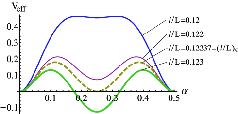
Figure 1: The behavior of the one-loop effective potential with respect to the ratio ${l\over L}=0.12,0.122,0.12237,0.123$ with $z=2$. According to the change of the ratio, the vacuum configuration changes from $\alpha=0$ (mod $1/2$) to $\alpha=0.25$. The degenerate vacuum appears at the critical ratio $({l\over L})_{c}=0.12237$, above which the vacuum configuration is $\alpha=0.25$, where gauge symmetry is broken down to $U(1)$.

Actually, the vacuum structure changes according to the magnitude of $l/L$, as shown in Fig.$1$. We find that for $z=2$ the degenerate vacuum appear at the critical ratio,

$$\left({l\over L}\right)_{c}=0.12237.$$ (51)

For larger value than the critical ratio, the $SU(2)$ gauge symmetry is broken to $U(1)$, while the smaller value than the critical value, the $SU(2)$ gauge symmetry is unbroken. The behavior of the vacuum expectation value (VEV) $\alpha$ with respect to $l/L$ is depicted in Fig.$2$, where we observe that the VEV jumps at the critical ratio, hence the phase transition is first order.

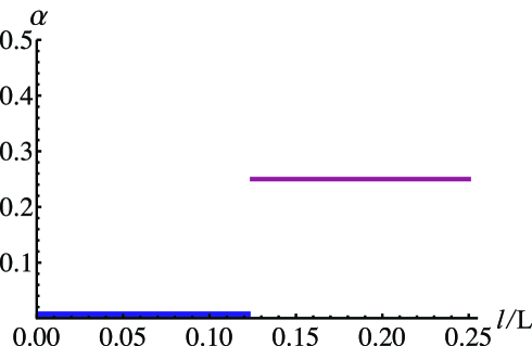
Figure 2: The behavior of the vacuum expectation value (VEV) $\alpha$ with respect to ${l\over L}$. At the critical ratio $({l\over L})_{c}=0.12237$, the VEV jumps, and the phase transition is first order.

Let us next discuss the mass of the adjoint scalar field which is originally the component gauge field for the $S^{1}$ direction. The mass of the adjoint Higgs scalar is obtained by the second derivative of the effective potential evaluated at the vacuum,

$$m_{H}^{2} = {\partial^{2}V_{\textrm{eff}}^{R^{4}\times S^{1}_{z}}(\alpha)\over\partial\langle A_{y}^{3}\rangle^{2}}\bigg{|}_{\rm vac}=\left({gL\over 4\pi}\right)^{2}~{}{\partial^{2}V_{\textrm{eff}}^{R^{4}\times S^{1}_{z}}(\alpha)\over\partial\alpha^{2}}\bigg{|}_{\rm vac}$$ (52)

$$= {3~{}{\bar{g}}^{2}\over 2\pi^{2}L^{2}}\biggl{[}3\sum_{n=1}^{\infty}{1\over n^{3}}\cos(2\pi n(2\alpha))$$

$$-4z{\Gamma(4z+1)\over\Gamma(5)}\biggl{(}{l\over L}\biggr{)}^{4(z-1)}~{}\sum_{n=1}^{\infty}{1\over n^{4z-1}}\cos(2\pi n(2\alpha))\biggr{]}\bigg{|}_{\rm vac}.$$

where we have defined the 4d gauge coupling constant ${\bar{g}}\equiv g/\sqrt{L}$. Hereafter we take $z=2$ for numerical studies.

Let us study the case of $\alpha=0.25$, for which the gauge symmetry is broken to $U(1)$. The adjoint Higgs mass is given by

$$m_{H}^{2}={3~{}{\bar{g}}^{2}\over 2\pi^{2}L^{2}}\biggl{[}-{9\over 4}~{}\zeta(3)+4\times 2\times{8!\over 4!}\left({l\over L}\right)^{4}\times{63\over 64}~{}\zeta(7)\biggr{]},$$ (53)

where we have used the Riemann’s zeta function,

$$\sum_{n=1}^{\infty}{(-1)^{n}\over n^{4k-1}}=-(1-2^{2-4k})\zeta(4k-1)$$ (54)

with $k=1,2$. The mass squared $m_{H}^{2}$ is positive definite for the range of $(l/L)_{c}<l/L$, where the vacuum configuration is given by $\alpha=0.25$. We note that the Gamma function $\Gamma(4z+1)$ is sizable enhancement for the mass. The adjoint scalar mass depends on the ratio $l/L$, which can also enhance the mass of the adjoint scalar field.

The ratio between the adjoint Higgs scalar and the lightest massive gauge boson is given by

$${m_{H}\over M_{W}^{(0)}}={\bar{g}}\sqrt{{3\over 2\pi^{4}}\left(-{9\over 4}\zeta(3)+13230\times\zeta(7)\times\biggl{(}{l\over L}\biggr{)}^{4}\right)},$$ (55)

where we have used the expression for the the massive Kaluza-Klein gauge bosons after the gauge symmetry breaking,

$$M_{W}^{(n)2}=\left(2\pi\over L\right)^{2}\left(n+2\alpha\right)^{2}\Bigg{|}_{\alpha=0.25}\quad\mbox{for}\quad n=0,1,2,\cdots.$$ (56)

We obtain the mass of the adjoint Higgs scalar field for various values of $l/L$

$${m_{H}\over M_{W}^{(0)}}={\bar{g}}\times\left\{\begin{array}[]{cl}0.54&\mbox{for}~{}~{}{l\over L}=0.2,\\[5.69046pt] 2.28&\mbox{for}~{}~{}{l\over L}=0.4,\\[5.69046pt] 9.17&\mbox{for}~{}~{}{l\over L}=0.8,\\[5.69046pt] 14.3&\mbox{for}~{}~{}{l\over L}=1.0,\\[5.69046pt] 20.6&\mbox{for}~{}~{}{l\over L}=1.2,\\[5.69046pt] \end{array}\right.$$ (57)

The adjoint Higgs mass is generated through loop effects and is natural to be light compared with the massive gauge boson appeared after the gauge symmetry breaking. In the present case, however, thanks to the arbitrary scale $l$ and the Gamma function $\Gamma(4z+1)$, the adjoint scalar mass can be heavier than the massive gauge boson, as shown above.

The Higgs mass is also affected by the dynamical critical exponent $z$. In order to see it, let us study the ratio between the adjoint Higgs scalar and the lightest massive gauge boson with respect to $z$ for fixed value of $l/L$. We take $l/L=0.25$ as an illustration, for which the $SU(2)$ gauge symmetry is broken to $U(1)$. We obtain, from (52) and (56), that

$${m_{H}\over M_{W}^{(0)}}={\bar{g}}\times\left\{\begin{array}[]{cl}0.12&\mbox{for}~{}~{}z=1,\\[5.69046pt] 0.87&\mbox{for}~{}~{}z=2,\\[5.69046pt] 7.50&\mbox{for}~{}~{}z=3,\\[5.69046pt] 113.15&\mbox{for}~{}~{}z=4.\\[5.69046pt] \end{array}\right.$$ (58)

We observe that the Higgs mass highly depends on $z$ and is enhanced by the effect of the higher derivative, as pointed out in the previous section.

5 Higher Dimensional Extension

In this section, we extend the previous analysis in section 3 to the Lifshitz type gauge theory on $R^{D-2}\times S^{1}_{z_{1}}\times S^{1}_{z_{2}}$, and show that the effective potential on $R^{D-2}\times S^{1}_{z_{1}}\times S^{1}_{z_{2}}$ is given by the sum of an effective potential on $R^{D-2}\times R^{1}_{z_{1}}\times S^{1}_{z_{2}}$ and infinitely many effective potentials for Kaluza-Klein modes on $R^{D-2}\times S^{1}_{z_{1}}$. We here focus on a massless scalar contribution to the one-loop effective potential

$$V^{R^{D-2}\times S^{1}_{z_{1}}\times S^{1}_{z_{2}}}_{\textrm{scalar}}(\alpha_{1},\alpha_{2};M_{S}=0)$$

$$\qquad=-\Bigl{(}\frac{1}{4\pi}\Bigr{)}^{(D-2)/2}\Bigl{(}\frac{1}{L_{1}}\sum^{\infty}_{m_{1}=-\infty}\Bigr{)}\Bigl{(}\frac{1}{L_{2}}\sum^{\infty}_{m_{2}=-\infty}\Bigr{)}\int^{\infty}_{0}dt\,t^{-D/2}$$

$$\qquad\quad\times\textrm{tr}_{(\cal{R})}\biggl{[}\exp\Bigl{\{}-t\Bigl{[}l_{1}^{2(z_{1}-1)}\Bigl{(}\frac{2\pi(m_{1}+\alpha_{1})}{L_{1}}\Bigr{)}^{2z_{1}}+l_{2}^{2(z_{2}-1)}\Bigl{(}\frac{2\pi(m_{2}+\alpha_{2})}{L_{2}}\Bigr{)}^{2z_{2}}\Bigr{]}\Bigr{\}}\biggr{]}\,,$$ (59)

where the scalar action has been assumed to include $l_{1}^{2(z_{1}-1)}(D_{y_{1}})^{2z_{1}}$ and $l_{2}^{2(z_{2}-1)}(D_{y_{2}})^{2z_{2}}$ for $S^{1}_{z_{1}}$ and $S^{1}_{z_{2}}$ directions, respectively. The $L_{1}$ and $L_{2}$ are the circumferences of $S^{1}_{z_{1}}$ and $S^{1}_{z_{2}}$, and $\alpha_{1}$ and $\alpha_{2}$ are defined by $\alpha_{1}=g\langle A_{y_{1}}\rangle L_{1}/(2\pi)$ and $\alpha_{2}=g\langle A_{y_{2}}\rangle L_{2}/(2\pi)$. We note that $\alpha_{1}$ and $\alpha_{2}$ are assumed to commute each other to minimize the tree level potential $g^{2}\textrm{tr}_{(\textrm{adj})}[A_{y_{1}},A_{y_{2}}]^{2}$. Using the Poisson summation formula (14), we obtain the UV finite expression

$$V^{R^{D-2}\times S^{1}_{z_{1}}\times S^{1}_{z_{2}}}_{\textrm{scalar}}(\alpha_{1},\alpha_{2};M_{S}=0)$$

$$\qquad=-\Bigl{(}\frac{1}{4\pi}\Bigr{)}^{\frac{D-2}{2}}\frac{1}{L_{1}L_{2}}\sum^{\infty}_{n_{1},n_{2}=-\infty}{}^{\prime}\hskip 5.69054pt\int_{0}^{\infty}dt\,t^{-D/2}\int_{-\infty}^{\infty}du_{1}\int_{-\infty}^{\infty}du_{2}$$

$$\qquad\quad\times\textrm{tr}_{(\cal{R})}\biggl{[}\exp\Bigl{\{}-t\Bigl{[}l_{1}^{2(z_{1}-1)}\Bigl{(}\frac{2\pi u_{1}}{L_{1}}\Bigr{)}^{2z_{1}}+l_{2}^{2(z_{2}-1)}\Bigl{(}\frac{2\pi u_{2}}{L_{2}}\Bigr{)}^{2z_{2}}\Bigr{]}$$

$$\qquad\quad-2\pi i\bigl{(}n_{1}u_{1}+n_{2}u_{2}\bigr{)}+2\pi i\bigl{(}n_{1}\alpha_{1}+n_{2}\alpha_{2}\bigr{)}\Bigr{\}}\biggr{]}\,,$$ (60)

where the prime of the summation denotes that the contribution of $n_{1}=n_{2}=0$ has to be removed from the summation to subtract the UV divergent part from the effective potential. The summation over $n_{1}$ and $n_{2}$ may be rearranged as follows:

$$\sum_{n_{1},n_{2}=-\infty}^{\infty}{}^{\prime} \equiv\sum_{n_{1}=-\infty}^{\infty}\sum_{n_{2}=-\infty}^{\infty}\bigl{(}1-\delta_{n_{1},0}\delta_{n_{2},0}\bigr{)}$$

$$=\sum_{n_{1}=-\infty}^{\infty}\sum_{n_{2}=-\infty}^{\infty}\bigl{\{}\delta_{n_{1},0}\bigl{(}1-\delta_{n_{2},0}\bigr{)}+\bigl{(}1-\delta_{n_{1},0}\bigr{)}\bigr{\}}$$

$$=\sum_{n_{1}=-\infty}^{\infty}\delta_{n_{1},0}\sum_{n_{2}=-\infty}^{\infty}{}^{\prime}+\sum_{n_{1}=-\infty}^{\infty}{}^{\prime}\ \sum_{n_{2}=-\infty}^{\infty}\,.$$ (61)

Thus, we can rewrite Eq.(5) as

$$V^{R^{D-2}\times S^{1}_{z_{1}}\times S^{1}_{z_{2}}}_{\textrm{scalar}}(\alpha_{1},\alpha_{2};M=0)$$

$$\qquad=-\Bigl{(}\frac{1}{4\pi}\Bigr{)}^{\frac{D-2}{2}}\frac{1}{L_{1}L_{2}}\sum^{\infty}_{n_{2}=-\infty}{}^{\!\!\!\!\prime}\int_{0}^{\infty}dt\,t^{-D/2}\int_{-\infty}^{\infty}du_{1}\int_{-\infty}^{\infty}du_{2}$$

$$\qquad\qquad\times\textrm{tr}_{(\cal{R})}\biggl{[}\exp\Bigl{\{}-t\Bigl{[}l_{1}^{2(z_{1}-1)}\Bigl{(}\frac{2\pi u_{1}}{L_{1}}\Bigr{)}^{2z_{1}}+l_{2}^{2(z_{2}-1)}\Bigl{(}\frac{2\pi u_{2}}{L_{2}}\Bigr{)}^{2z_{2}}\Bigr{]}$$

$$\qquad\qquad-2\pi in_{2}u_{2}+2\pi in_{2}\alpha_{2}\Bigr{\}}\biggr{]}$$

$$\qquad-\Bigl{(}\frac{1}{4\pi}\Bigr{)}^{\frac{D-2}{2}}\frac{1}{L_{1}L_{2}}\sum^{\infty}_{n_{1}=-\infty}{}^{\!\!\!\!\prime}\ \sum^{\infty}_{n_{2}=-\infty}\int_{0}^{\infty}dt\,t^{-D/2}\int_{-\infty}^{\infty}du_{1}\int_{-\infty}^{\infty}du_{2}$$

$$\qquad\qquad\times\textrm{tr}_{(\cal{R})}\biggl{[}\exp\Bigl{\{}-t\Bigl{[}l_{1}^{2(z_{1}-1)}\Bigl{(}\frac{2\pi u_{1}}{L_{1}}\Bigr{)}^{2z_{1}}+l_{2}^{2(z_{2}-1)}\Bigl{(}\frac{2\pi u_{2}}{L_{2}}\Bigr{)}^{2z_{2}}\Bigr{]}$$

$$\qquad\qquad-2\pi i\bigl{(}n_{1}u_{1}+n_{2}u_{2}\bigr{)}+2\pi i\bigl{(}n_{1}\alpha_{1}+n_{2}\alpha_{2}\bigr{)}\Bigr{\}}\biggr{]}\,.$$ (62)

The first term on the r.h.s. of Eq.(5) can be expressed, with the change of variable $p_{1}=2\pi u_{1}/L_{1}$, as

$$-\Bigl{(}\frac{1}{4\pi}\Bigr{)}^{\frac{D-2}{2}}\frac{1}{L_{2}}\sum^{\infty}_{n_{2}=-\infty}{}^{\!\!\!\!\prime}\int_{0}^{\infty}dt\,t^{-D/2}\int_{-\infty}^{\infty}\frac{dp_{1}}{2\pi}\int_{-\infty}^{\infty}du_{2}$$

$$\qquad\quad\times\textrm{tr}_{(\cal{R})}\biggl{[}\exp\Bigl{\{}-t\Bigl{[}l_{1}^{2(z_{1}-1)}p_{1}^{2z_{1}}+l_{2}^{2(z_{2}-1)}\Bigl{(}\frac{2\pi u_{2}}{L_{2}}\Bigr{)}^{2z_{2}}\Bigr{]}-2\pi in_{2}u_{2}+2\pi in_{2}\alpha_{2}\Bigr{\}}\biggr{]}$$

$$\quad\equiv V^{R^{D-2}\times R^{1}_{z_{1}}\times S^{1}_{z_{2}}}_{\textrm{scalar}}(\alpha_{2};M=0)\,.$$ (63)

It turns out that $V^{R^{D-2}\times R^{1}_{z_{1}}\times S^{1}_{z_{2}}}_{\textrm{scalar}}(\alpha_{2};M=0)$ has a clear geometrical meaning. It is nothing but the one-loop effective potential of a $D$-dimensional Lifshitz type gauge theory on $R^{D-2}\times R^{1}_{z_{1}}\times S^{1}_{z_{2}}$ (but not $R^{D-2}\times S^{1}_{z_{1}}\times S^{1}_{z_{2}}$) where a Lifshitz type higher derivative labeled by $z_{1}$ appears for one of the coordinates in $R^{D-1}$ (i.e. $R^{1}_{z_{1}}$) as well as for the coordinate of $S^{1}_{z_{2}}$.

The second term on the r.h.s. of Eq.(5) can be expressed, by using the Poisson summation formula reversely, as

$$\frac{1}{L_{2}}\sum_{m_{2}=-\infty}^{\infty}\frac{-1}{(4\pi)^{(D-2)/2}}\frac{1}{L_{1}}\sum^{\infty}_{n_{1}=-\infty}{}^{\!\!\!\!\prime}\ \int_{0}^{\infty}dt\,t^{-D/2}\int_{-\infty}^{\infty}du_{1}$$

$$\qquad\qquad\times\textrm{tr}_{(\cal{R})}\biggl{[}\exp\Bigl{\{}-t\Bigl{[}l_{1}^{2(z_{1}-1)}\Bigl{(}\frac{2\pi u_{1}}{L_{1}}\Bigr{)}^{2z_{1}}+M_{m_{2}}^{\ 2}\Bigr{]}-2\pi in_{1}u_{1}+2\pi in_{1}\alpha_{1}\Bigr{\}}\biggr{]}$$

$$\quad\equiv\frac{1}{L_{2}}\sum_{m_{2}=-\infty}^{\infty}V^{R^{D-2}\times S^{1}_{z_{1}}}_{\textrm{scalar}}(\alpha_{1};M_{m_{2}})\,,$$ (64)

where

$$M_{m_{2}}\equiv l_{2}^{\,z_{2}-1}\Bigl{|}\frac{2\pi(m_{2}+\alpha_{2})}{L_{2}}\Bigr{|}^{z_{2}}\,.$$ (65)

Again, $V^{R^{D-2}\times S^{1}_{z_{1}}}_{\textrm{scalar}}(\alpha_{1};M_{m_{2}})$ turns out to have a clear geometrical meaning. It is nothing but the one-loop effective potential of a $(D-1)$-dimensional Lifshitz type gauge theory (but not $D$-dimensional one) on $R^{D-2}\times S^{1}_{z_{1}}$ where the scalar action contains the Lifshitz type higher derivative of $z_{1}$ for the $S^{1}_{z_{1}}$ direction with the bulk mass $M_{m_{2}}$ that corresponds to the Kaluza-Klein mass of the mode $m_{2}$. Thus, we found that

$$V^{R^{D-2}\times S^{1}_{z_{1}}\times S^{1}_{z_{2}}}_{\textrm{scalar}}(\alpha_{1},\alpha_{2};M=0)$$

$$\quad=V^{R^{D-2}\times R^{1}_{z_{1}}\times S^{1}_{z_{2}}}_{\textrm{scalar}}(\alpha_{2};M=0)+\frac{1}{L_{2}}\sum_{m_{2}=-\infty}^{\infty}V^{R^{D-2}\times S^{1}_{z_{1}}}_{\textrm{scalar}}(\alpha_{1};M_{m_{2}})\,.$$ (66)

Since the above observation is expected to hold for fermion and gauge fields, the one-loop effective potential of the Lifshitz type gauge theory on $R^{D-2}\times S^{1}_{z_{1}}\times S^{1}_{z_{2}}$ turns out be written into a decomposition form similar to Eq.(5). We also expect that the effective potential for a Lifshitz type gauge theory on $R^{D-N}\times S^{1}_{z_{1}}\times\cdots\times S^{1}_{z_{N}}$ has a similar structure, though we will not proceed furthermore.

6 Conclusions and Discussions

We have investigated the Lifshitz type gauge theory in the gauge-Higgs unification. The Lifshitz scalar and fermion possess the kinetic terms of the higher derivatives labeled by $z$ for the direction of the extra dimension. We have succeeded to evaluate the one-loop effective potential for the zero mode of the extra dimensional component of the gauge field and found that it heavily depends on the dynamical critical exponent $z$ of the Lifshitz particles. The overall sign of the effective potential can change with respect to $z$ irrespective of the spin and statistics, and furthermore the one-loop effective potential turns out to vanish for even $D$ and $z$. A huge numerical factor arises for $z>1$ and this property may solve the light Higgs mass problem. It has also been found that the length parameter $l$ plays an important role in determining the vacuum expectation value of the Higgs field as well as the magnitude of the Higgs mass.

To obtain the finite expression of the one-loop effective potential, we have extended the space-time dimension $D$ to a real (or complex) number and taken it to be the original integral value only at the final stage. To confirm this procedure, we have provided the mathematical tools and derived the one-loop effective potential in the several different ways. We have also studied the one-loop effective potentials numerically in the 5d $SU(2)$ model, and confirmed various peculiar properties of our models.

The analysis for the Lifshitz type gauge theory on $R^{D-1}\times S^{1}_{z}$ has been extended to the higher extra dimensions $S^{1}_{z_{1}}\times S^{1}_{z_{2}}$. An interesting observation is that the one-loop effective potential on $R^{D-2}\times S^{1}_{z_{1}}\times S^{1}_{z_{2}}$ can be expressed by the sum of a one-loop effective potential on $R^{D-2}\times R^{1}_{z_{1}}\times S^{1}_{z_{2}}$ and infinitely many one-loop ones on $R^{D-2}\times S^{1}_{z_{1}}$, which is one-dimension lower than the original space-time dimension $D$, coming from Lifshitz Kaluza-Klein particles on $S^{1}_{z_{2}}$. A similar decomposition property will hold for the Lifshitz type gauge theory on the higher extra dimension $S^{1}_{z_{1}}\times S^{1}_{z_{2}}\times\cdots\times S^{1}_{z_{N}}$.

Another extension is to replace the circle $S_{z}^{1}$ with the orbifold $S_{z}^{1}/Z_{2}$. We can apply the methods developed here to this case. Hence, it is important and interesting to study the gauge symmetry breaking and Higgs mass in a context of Lifshitz type gauge theories on $S_{z}^{1}/Z_{2}$.

In this paper, we have assumed the higher derivative terms to present only for the direction of the extra dimensions. Hořava’s original idea [18] is, however, to demand the anisotropy between time and space coordinates to make gravity theory power-counting renormalizable. According to the Hořava’s spirit, we may replace the second order derivatives of all the spatial coordinates of $R^{D-1}\times S^{1}$ by higher derivatives to make the theory renormalizable. The power-counting renormalizability requires the mass dimension of the gauge coupling to be non-negative. This implies that the dynamical critical exponent $z$ should be greater than or equal to $D-3$. The one-loop effective potential coming from such a Hořava-Lifshitz massless scalar loop may be given by

$$V^{R^{1}\times R^{D-2}_{z}\times S^{1}_{z}}_{\textrm{scalar}}(\alpha;M=0)$$

$$\qquad=-\int\frac{d^{D-2}\bm{p}}{(2\pi)^{D-2}}\frac{1}{L}\sum^{\infty}_{m=-\infty}\int^{\infty}_{0}dt\,t^{-1}\frac{1}{\sqrt{4\pi t}}$$

$$\qquad\qquad\times\textrm{tr}_{(\cal{R})}\biggl{[}\exp\Bigl{\{}-t\,l^{2(z-1)}\Bigl{(}\bigl{(}\bm{p}^{2}\bigr{)}^{z}+\Bigl{(}\frac{2\pi(m+\alpha)}{L}\Bigr{)}^{2z}\Bigr{)}\Bigr{\}}\biggr{]}$$

$$\qquad=-2z\Bigl{(}\frac{1}{\pi}\Bigr{)}^{1/2}C_{z}\frac{\sin\bigl{(}\pi(z+D-2)/2\bigr{)}\Gamma\bigl{(}z+D-2\bigr{)}}{\sin\bigl{(}\pi(z+D-2)/(2z)\bigr{)}\Gamma\bigl{(}(z+D-2)/(2z)\bigr{)}}$$

$$\qquad\qquad\times\frac{1}{L^{D}}\Bigl{(}\frac{l}{L}\Bigr{)}^{z-1}\sum_{n=1}^{\infty}\textrm{tr}_{({\cal R})}\biggl{[}\frac{\cos(2\pi n\alpha)}{n^{z+D-1}}\biggr{]}\,,$$ (67)

where

$$C_{z}\equiv\int\frac{d^{D-2}\bm{p}}{(2\pi)^{D-2}}\ e^{-(\bm{p}^{2})^{z}}.$$ (68)

We should emphasize that standard gauge-Higgs unification models are not renormalizable because the total space-time dimension $D$ is greater than 4. Thus, only a very limited class of physical quantities such as the Higgs mass are finite and calculable, so that the predictability of the theory is quite restricted. Since the Hořava-Lifshitz type gauge theory is power-counting renormalizable, any physical quantities can, in principle, be computed with finite values at the cost of Lorentz symmetry violation. It would be of great interest to investigate Hořava-Lifshitz type gauge theory in more details.

Acknowledgement

This work is supported in part by a Grant-in-Aid for Scientific Research (No. 22540281 and No. 20540274 (M.S.), No. 21540285 (K.T.)) from the Japanese Ministry of Education, Science, Sports and Culture. The authors would like to thank Professors M. Kato, N. Maru and H. So for valuable discussions.

Appendix A Other Methods to Evaluate the Effective Potential

In the followings, we show the alternative ways to reproduce the result (3.1).

A.1 A method with contour Integrals

Eq. (3.1) can be reproduced in a way similar to [38]. First, in terms of contour integrals, Eq. (26) can be written as

$$V_{\rm scalar}^{R^{D-1}\times S_{z}^{1}}(\alpha;M_{S}=0)$$

$$= -\frac{\Gamma\left(-{D-1\over 2}\right)}{(4\pi)^{(D-1)\over 2}}\frac{l^{(z-1)(D-1)}}{L}\left(\frac{2\pi}{L}\right)^{z(D-1)}\frac{1}{2\pi i}\textrm{tr}_{(\cal{R})}\oint_{C}dw\,w^{z(D-1)}\frac{dF(w,\alpha)/dw}{F(w,\alpha)}$$

$$= \frac{\Gamma\left(-{D-1\over 2}\right)}{(4\pi)^{(D-1)\over 2}}\frac{l^{(z-1)(D-1)}}{L}\left(\frac{2\pi}{L}\right)^{z(D-1)}\frac{z(D-1)}{2\pi i}\textrm{tr}_{(\cal{R})}\oint_{C}dw\,w^{z(D-1)-1}\ln[F(w,\alpha)],$$

where

$$F(w,\alpha) = \cos(2\pi w)-\cos(2\pi\alpha),$$ (70)

and the contour $C$ is the set of the circles each of which surrounds $w=m\pm\alpha>0$, $m=0,1,\cdots$, on the $w$-plane. Since the integrand is regular except for roots on the real axes, we can change a closed path of $\textrm{Re}~{}w>0$ to the contour shown in Fig. 3, where the closed path consists of the infinite semicircle on the plane $C_{1}$, the straight lines $C_{2}$ from $+i\infty$ to $+i\delta$ ($\delta$ is a positive infinitesimal) and $C_{4}$ from $-i\delta$ to $-i\infty$, and a semicircle $C_{3}$ centered at the origin with radius $\delta$ .

Figure 3: The integration path stretched on the positive-real plane.

The integrals along the infinite semicircle vanishes in the sense of analytic continuation and by taking the limit $\delta\to 0$, only integrals along $C_{2}$ and $C_{4}$ remain non-vanishing, and thus we obtain

$$V_{\rm scalar}^{R^{D-1}\times S_{z}^{1}}(\alpha;M_{S}=0)$$ (71)

$$= -\frac{\Gamma\left(-{D-1\over 2}\right)}{(4\pi)^{(D-1)\over 2}}\frac{l^{(z-1)(D-1)}}{L}\left(\frac{2\pi}{L}\right)^{z(D-1)}\frac{z(D-1)}{2\pi i}$$

$$\times{\text{tr}}_{({\cal R})}\biggl{[}-i^{z(D-1)}\int_{0}^{\infty}dt\,t^{z(D-1)-1}\ln[F(it,\alpha)]$$

$$\phantom{MM}+(-i)^{z(D-1)}\int_{0}^{\infty}dt\,t^{z(D-1)-1}\ln[F(-it,\alpha)]\biggr{]}$$

$$= \frac{\Gamma\left(-{D-1\over 2}\right)}{(4\pi)^{(D-1)\over 2}}\frac{l^{(z-1)(D-1)}}{L}\left(\frac{2\pi}{L}\right)^{z(D-1)}\frac{z(D-1)}{\pi}$$

$$\times\sin\left(\frac{\pi z(D-1)}{2}\right){\text{tr}}_{({\cal R})}{\cal J},$$

where we have used $F(w,\alpha)=F(-w,\alpha)$ and

$${\cal J}\equiv\int_{0}^{\infty}dt\,t^{z(D-1)-1}\ln[F(it,\alpha)].$$ (72)

Recalling a relation $\cosh(A)-\cos(B)=e^{A}(1-e^{-A+iB})(1-e^{-A-iB})/2$, we can rewrite ${\cal J}$ as

$${\cal J} = \int_{0}^{\infty}dt\,t^{z(D-1)-1}\left\{\ln(1-e^{-2\pi t+i2\pi\alpha})+\ln(1-e^{-2\pi t-i2\pi\alpha})+2\pi t-\ln(2)\right\}.$$ (73)

We note that the above integral contains divergences. We ignore such divergent terms because we are interested in $\alpha$-dependent ones. Using the expansion formula

$$\ln(1-e^{-2\pi t+i2\pi n\alpha}) = -\sum_{n=1}^{\infty}\frac{e^{-2\pi nt+i2\pi n\alpha}}{n},$$ (74)

and after integration we get

$${\cal J} = -\frac{2}{(2\pi)^{z(D-1)}}\Gamma(z(D-1))\sum_{n=1}^{\infty}\frac{\cos(2\pi n\alpha)}{n^{z(D-1)+1}}.$$ (75)

Combining (71) and (75), and utilizing the Gamma function formulas, one can reproduce the same result as (3.1).

A.2 Use of Hypergeometric Functions

Here we show the one more way to evaluate the effective potential. Using Poisson summation, we can write (3.1) as

$$V_{\rm scalar}^{R^{D-1}\times S_{z}^{1}}(\alpha;M_{S}=0)$$ (76)

$$= -\frac{\sqrt{2\pi}(2\pi)^{z(D-1)}}{(4\pi)^{\frac{D-1}{2}}}{1\over L}\left(\frac{l^{z-1}}{L^{z}}\right)^{D-1}\textrm{tr}_{(\cal{R})}\sum_{n=-\infty}^{\infty}e^{i2\pi n\alpha}\int_{0}^{\infty}d\tau\,\tau^{-\frac{D-1}{2}-1}F_{2z}\left(2\pi n;\tau\right),$$

where

$$F_{2z}(y;\tau)\equiv\frac{1}{\sqrt{2\pi}}\int_{-\infty}^{\infty}dx\,\exp[-\tau x^{2z}]e^{ixy}$$ (77)

and we have used the following Poisson summation formula

$$\sum_{m=-\infty}^{\infty}\exp\left[-\tau(m+\alpha)^{2z}\right] = \sqrt{2\pi}\sum_{n=-\infty}^{\infty}e^{i2\pi n\alpha}F_{2z}\left(2\pi n;\tau\right).$$ (78)

We can rewrite $F_{2z}(y;\tau)$ into the form

$$F_{2z}(y;\tau)=\frac{1}{\sqrt{2\pi}z\tau^{1/(2z)}}\sum_{r=0}^{\infty}\frac{\displaystyle\left(\frac{iy}{\tau^{1/(2z)}}\right)^{2r}}{(2r)!}\Gamma\Bigl{(}\frac{2r+1}{2z}\Bigr{)}\,,$$ (79)

where we have expanded $e^{ixy}$ in powers of $x$ and used the integral representation of the gamma function. To proceed further, we note that any non-negative integer $r$ can uniquely be parameterized by two integers $s$ and $k$ such that $r=zs+k$, where $r=0,1,2,\cdots$, $s=0,1,2,\cdots$ and $k=0,1,\cdots,z-1$. In terms of the Pochhammer’s symbol

$$(a)_{s}\equiv a(a+1)(a+2)\cdots(a+s-1)=\frac{\Gamma(a+s)}{\Gamma(a)}\,,$$ (80)

we have

$$\Gamma\Bigl{(}\frac{2r+1}{2z}\Bigr{)} =\Gamma\Bigl{(}\frac{2zs+2k+1}{2z}\Bigr{)}=\Bigl{(}\frac{2k+1}{2z}\Bigr{)}_{\!s}\Gamma\Bigl{(}\frac{2k+1}{2z}\Bigr{)}\,,$$ (81)

$$(2r)! =(2zs+2k)!=(2k)!\,\Bigl{(}\frac{2k+1}{2z}\Bigr{)}_{\!s}\Bigl{(}\frac{2k+2}{2z}\Bigr{)}_{\!s}\cdots\Bigl{(}\frac{2k+2z}{2z}\Bigr{)}_{\!s}\,(2z)^{2zs}\,.$$ (82)

It then follows that

$$F_{2z}(y;\tau)= \frac{1}{\sqrt{2\pi}z\tau^{1/(2z)}}\sum_{k=0}^{z-1}\frac{\Gamma\bigl{(}\frac{2k+1}{2z}\bigr{)}}{(2k)!}\Bigl{(}\frac{iy}{\tau^{1/(2z)}}\Bigr{)}^{2k}$$

$$\qquad\qquad\times{}_{1}F_{2z-1}\Bigl{(}1;\frac{2k+2}{2z},\frac{2k+3}{2z},\cdots,\frac{2k+2z}{2z};\Bigl{(}\frac{iy}{2z}\Bigr{)}^{2z}\frac{1}{\tau}\Bigr{)}\,,$$ (83)

where we have used the relation $(1)_{s}=s!$ and ${}_{p}F_{q}(\cdots)$ is the generalized hypergeometric function defined by

$${}_{p}F_{q}(a_{1},\cdots,a_{p};b_{1},\cdots,b_{q};w) \equiv \sum_{s=0}^{\infty}\frac{(a_{1})_{s}(a_{2})_{s}\cdots(a_{p})_{s}}{(b_{1})_{s}(b_{2})_{s}\cdots(b_{q})_{s}}\frac{w^{s}}{s!}\,.$$ (84)

Truncating the $n=0$ mode, which is independent to $\alpha$ and responsible for the UV divergence, and integrating with respect to $\tau$, we obtain

$$V_{\rm scalar}^{R^{D-1}\times S_{z}^{1}}(\alpha;M_{S}=0)$$ (85)

$$= -\frac{2\sqrt{2\pi}(2\pi)^{z(D-1)}}{(4\pi)^{\frac{D-1}{2}}}\frac{1}{L}\left(\frac{l^{z-1}}{L^{z}}\right)^{D-1}\textrm{tr}_{(\cal{R})}\sum_{n=1}^{\infty}\cos(2\pi n\alpha)G_{2z}(2\pi n,D),$$

where $G_{2z}(y,D)$ is defined by

$$G_{2z}(y,D) \equiv \int_{0}^{\infty}d\tau\,\tau^{-\frac{D}{2}-\frac{1}{2}}F_{2z}(y;\tau).$$ (86)

By use of the formulas of an indefinite integral and an asymptotic expansion of generalized hypergeometric functions

$$\int du\,u^{\alpha-1}\,{}_{p}F_{q}(a_{1},\cdots,a_{p};b_{1},\cdots,b_{q};u)$$

$$\hskip 85.35826pt=\frac{u^{\alpha}}{\alpha}\,{}_{p+1}F_{q+1}(\alpha,a_{1},\cdots,a_{p};\alpha+1,b_{1},\cdots,b_{q};u),$$ (87)

$${}_{p}F_{q}(a_{1},\cdots,a_{p};b_{1},\cdots,b_{q};u)$$

$$\hskip 85.35826pt\stackrel{{\scriptstyle|u|\rightarrow\infty}}{{\longrightarrow}}\ \ \sum_{k=1}^{p}\frac{\Gamma(a_{k})\left(\prod_{j=1}^{q}\Gamma(b_{j})\right)\prod_{j=1,j\neq k}^{p}\Gamma(a_{j}-a_{k})}{\left(\prod_{j=1}^{p}\Gamma(a_{j})\right)\prod_{j=1}^{q}\Gamma(b_{j}-a_{k})}(-u)^{-a_{k}},$$ (88)

we can show after some calculations that

$$G_{2z}(y,D)=\frac{2^{D-1/2}}{y^{z(D-1)+1}}\ \frac{\Gamma(D/2)\Gamma(z(D-1)+1)}{\Gamma(D)}\ \frac{\sin\bigl{(}\frac{z(D-1)}{2}\pi\bigr{)}}{\sin\bigl{(}\frac{(D-1)}{2}\pi\bigr{)}}.$$ (89)

Inserting it into Eq. (85) leads to Eq. (3.1), as expected.

Appendix B Effective Potential for Massive Matter

In this appendix we show the calculation for (3.2) in detail. Let us start with

$$V_{\rm scalar}^{R^{D-1}\times S_{z}^{1}}(\alpha,M)$$ (90)

$$= \int\frac{d^{D-1}p_{E}}{(2\pi)^{D-1}}\ \frac{1}{L}\sum^{\infty}_{m=-\infty}\textrm{tr}_{(\cal{R})}\biggl{[}\ln\Bigl{(}p_{E}^{\ 2}+l^{2(z-1)}\Bigl{(}\frac{2\pi(m+\alpha)}{L}\Bigr{)}^{2z}+M^{2}\Bigr{)}\biggr{]}$$

$$= \frac{2(\sqrt{\pi})^{D-1}}{(2\pi)^{D-1}\Gamma(\frac{D-1}{2})}\frac{1}{L}$$

$$\times\sum_{m=-\infty}^{\infty}\int_{M}^{\infty}dE\,E(\sqrt{E^{2}-M^{2}})^{D-3}{\rm tr}_{({\cal R})}\ln\left[E^{2}+l^{2z-2}\left(\frac{2\pi(m+\alpha)}{L}\right)^{2z}\right].$$

For odd $D$, we can write

$$V_{\rm scalar}^{R^{D-1}\times S_{z}^{1}}(\alpha,M)=\frac{2(\sqrt{\pi})^{D-1}}{(2\pi)^{D-1}\Gamma(\frac{D-1}{2})}\frac{1}{L}\sum_{q=0}^{\frac{D-3}{2}}{}_{\frac{D-3}{2}}C_{q}\,(-M^{2})^{\frac{D-3}{2}-q}\cdot I_{q},$$ (91)

where ${}_{n}C_{k}\equiv n!/(k!(n-k)!)$ is the binomial coefficient. $I_{q}$ is given by

$$I_{q} \equiv \sum_{m=-\infty}^{\infty}\int_{M}^{\infty}dE\,E^{2q+1}{{\text{tr}}}_{({\cal R})}\ln\left[E^{2}+l^{2z-2}\left(\frac{2\pi(m+\alpha)}{L}\right)^{2z}\right]$$ (92)

$$= \left(\frac{l^{z-1}}{L^{z}}\right)^{2q+2}\int_{ML^{z}/l^{z-1}}^{\infty}dQ~{}~{}Q^{2q+1}{\text{tr}}_{({\cal R})}W,$$

where

$$W\equiv\sum_{m=-\infty}^{\infty}\ln\left[Q^{2}+(2\pi(m+\alpha))^{2z}\right].$$ (93)

Here we have ignored $\alpha$-independent terms. Since the derivative $dW/dQ$ is given by

$$\frac{dW}{dQ} = \sum_{m=-\infty}^{\infty}\frac{2Q}{Q^{2}+(2\pi(m+\alpha))^{2z}}=\sum_{j=1}^{2z}\frac{G^{\prime}_{j}(Q)}{G_{j}(Q)},$$ (94)

$$G_{j}(Q) \equiv \sin\left(\pi\alpha-\frac{\omega_{j}Q^{1/z}}{2}\right),$$ (95)

$$\omega_{j} \equiv \exp\left(\frac{i(2j-1)\pi}{2z}\right),$$ (96)

(the derivation of (94) is given in the latter part of this appendix), we obtain

$$W = \ln\left[\prod_{j=1}^{2z}G_{j}(Q)\right]$$ (97)

$$= \ln\biggl{[}\prod_{j=1}^{z}\sin\left(\pi\biggl{(}\alpha-\frac{Q^{1/z}\omega_{j}}{2\pi}\biggr{)}\right)\sin\biggl{(}\pi\biggl{(}\alpha-\frac{Q^{1/z}\omega_{j}^{*}}{2\pi}\biggr{)}\biggr{)}\biggr{]},$$

$$= \ln\biggl{[}\frac{1}{4^{z}}\prod_{j=1}^{z}\exp(s_{j}Q^{1/z})\left\{1-\exp[-Q^{1/z}s_{j}+i(2\pi\alpha-Q^{1/z}c_{j})]\right\}$$

$$\quad\times\left\{1-\exp[-Q^{1/z}s_{j}-i(2\pi\alpha-Q^{1/z}c_{j})]\right\}\biggr{]},$$

where we have used the relation $\omega_{j}=\omega_{2z+1-j}^{*}$, and

$$s_{j} \equiv \mathop{\text{Im}}\nolimits\omega_{j}=\sin\left(\frac{i(2j-1)\pi}{2z}\right),$$ (98)

$$c_{j} \equiv \mathop{\text{Re}}\nolimits\omega_{j}=\cos\left(\frac{i(2j-1)\pi}{2z}\right).$$ (99)

Neglecting some $\alpha$-independent parts in $W$ which correspond to the ultraviolet divergences, we write $I_{q}$ as

$$I_{q} = {\text{tr}}_{({\cal R})}\left(\frac{l^{z-1}}{L^{z}}\right)^{2q+2}\sum_{j=1}^{z}2\mathop{\text{Re}}\nolimits J_{q,j},$$ (100)

$$J_{q,j} \equiv \int_{ML^{z}/l^{z-1}}^{\infty}dQ\,Q^{2q+1}\ln[1-\exp(-(s_{j}+ic_{j})Q^{1/z}+i2\pi\alpha)].$$ (101)

Using (74) and performing the integration of $J_{q,j}$, we get

$$J_{q,j} = -z(s_{j}+ic_{j})^{-z(2q+2)}\sum_{n=1}^{\infty}\frac{e^{i2\pi n\alpha}}{n^{z(2q+2)+1}}\Gamma(z(2q+2),n\rho_{j}),$$ (102)

where $\Gamma(x,y)\equiv\int_{y}^{\infty}t^{x-1}e^{-x}dx$ is the incomplete Gamma function and

$$\rho_{j}=(s_{j}+ic_{j})\left(\frac{ML^{z}}{l^{z-1}}\right)^{1/z}=\frac{i}{\omega_{j}}\left(\frac{ML^{z}}{l^{z-1}}\right)^{1/z}.$$

Combining (91), (100) and (102), we obtain

$$V_{\rm scalar}^{R^{D-1}\times S_{z}^{1}}(\alpha,M)$$ (103)

$$= -\frac{2(\sqrt{\pi})^{D-1}}{(2\pi)^{D-1}\Gamma(\frac{D-1}{2})}\frac{1}{L}\sum_{q=0}^{\frac{D-3}{2}}{}_{\frac{D-3}{2}}C_{q}(-M^{2})^{\frac{D-3}{2}-q}\left(\frac{l^{z-1}}{L^{z}}\right)^{2q+2}2z$$

$$\times{\text{tr}}_{({\cal R})}\sum_{j=1}^{z}\mathop{\text{Re}}\nolimits\Biggl{\{}\left(-i\omega_{j}\right)^{z(2q+2)}\sum_{n=1}^{\infty}\frac{e^{i2\pi n\alpha}}{n^{z(2q+2)+1}}\Gamma\left(z(2q+2),\frac{in}{\omega_{j}}\frac{LM^{1/z}}{l^{(z-1)/z}}\right)\Biggr{\}}.$$

One can rewrite (103) into more useful form. Utilizing an expansion formula $\Gamma(n,x)=(n-1)!e^{-x}\sum_{k=0}^{n-1}x^{k}/k!$, we can rewrite $J_{q,j}$ as

$$J_{q,j} = -z[z(2q+2)-1]!(-i\omega_{j})^{z(2q+2)}\sum_{n=1}^{\infty}\frac{e^{-n\rho_{j}+i2\pi n\alpha}}{n^{z(2q+2)+1}}\sum_{k=0}^{z(2q+2)-1}\frac{(n\rho_{j})^{k}}{k!}$$

$$= -z[z(2q+2)-1]!(-i\omega_{j})^{z(2q+2)}\sum_{k=0}^{z(2q+2)-1}\frac{(\rho_{j})^{k}}{k!}\mathop{\text{Li}}\nolimits_{z(2q+2)-k+1}(e^{-\rho_{j}+i2\pi\alpha}),$$

where we have changed the order of the summation and $\mathop{\text{Li}}\nolimits_{s}(x)$ is defined in (43). Combining (91), (100) and (B), we obtain (3.2).

Here we outline the derivation of (94). At first we point out that the left-hand-side of (94) can be written in terms of the following contour integral:

$$\sum_{m=-\infty}^{\infty}\frac{1}{x^{2z}+(2\pi(m+\alpha))^{2z}} = \frac{1}{2\pi i}\oint_{C_{\rm I}}dw\,\frac{\pi\cot(\pi w)}{x^{2z}+(2\pi(w+\alpha))^{2z}},$$ (105)

where the path $C_{\rm I}$ denotes the set of the circles surrounding the points $w=m$. Without changing the value of the integral, we can replace the integration path $C_{\rm I}$ by $C_{{\rm II}+}+C_{{\rm II}-}$ shown in Fig. 4.

Figure 4: Two contours $C_{{\rm II}\pm}$. $C_{{\rm II}+}$ ($C_{{\rm II}-}$) consists of the infinite semicircle above (below) the line $\mathop{\text{Im}}\nolimits(w)=0$, and the straight path from $+\infty+i\epsilon$ ($-\infty-i\epsilon$) to $-\infty+i\epsilon$ ($+\infty-i\epsilon$). $\epsilon$ denotes a positive infinitesimal.

Counting the residues of the integrand at the points which are enclosed by $C_{{\rm II}\pm}$, we obtain

$$\frac{1}{2\pi i}\oint_{C_{\rm I}}dw\,\frac{\pi\cot(\pi w)}{x^{2z}+(2\pi(w+\alpha))^{2z}} = -\sum_{j=1}^{2z}\mathop{\text{Res}}_{w\to\Omega_{j}}\left[\frac{\pi\cot(\pi w)}{x^{2z}+(2\pi(w+\alpha))^{2z}}\right],$$ (106)

$$= -\sum_{j=1}^{2z}\frac{\pi\cot\left(\pi\left(\frac{x\omega_{j}}{2\pi}-\alpha\right)\right)}{2\pi x^{2z-1}\displaystyle{\prod_{k=1,k\neq j}^{2z}}(\omega_{j}-\omega_{k})},$$

where $\Omega_{j}\equiv(x\omega_{j}-2\pi\alpha)/2\pi$, and $\mathop{\text{Res}}_{w\to a}[f(w)]$ denotes the residue of $f(w)$ at $w=a$. One can reproduce (94) by plugging $x=Q^{1/z}$ to (106) and using the formula

$${\prod_{k=1,k\neq j}^{2z}}(\omega_{j}-\omega_{k})=-\frac{2z}{\omega_{j}}.$$ (107)

References

- [1] M. S. Manton, Nucl. Phys. B158, 141 (1979).
- [2] D. B. Fairlie, Phys. Lett. B82, 97 (1979).
- [3] J. Sherk and J. Shwarz, Phys. Lett. B82, 60 (1979); Nucl. Phys. B153, 61 (1979).
- [4] Y. Hosotani, Phys. Lett. B126, 309 (1983), Ann. Phys. (N.Y.) 190, 233 (1989).
- [5] C. Csaki, C. Grojean, H. Murayama, L. Pilo and J. Terning, Phys. Rev. D69, 055006 (2004).
- [6] M. Sakamoto, M. Tachibana and K. Takenaga, Phys. Lett. B458, 231 (1999); Prog. Theor. Phys. 104, 633 (2000).
- [7] M. Sakamoto, M. Tachibana and K. Takenaga, Phys. Lett. B457, 33 (1999).
- [8] S. Matsumoto, M. Sakamoto and S. Tanimura, Phys. Lett. B518, 163 (2001); M. Sakamoto and S. Tanimura, Phys. Rev. D65, 065004 (2004).
- [9] H. Hatanaka, K. Ohnishi,M. Sakamoto and K. Takenaga, Prog. Theor. Phys. 107, 1191 (2002), Prog. Theor. Phys. 110, 791 (2003).
- [10] K. Ohnishi and M. Sakamoto, Phys. Lett. B486, 179 (2000); H. Hatanaka, S. Matsumoto, K. Ohnishi and M. Sakamoto, Phys. Rev. D63, 105003 (2001).
- [11] M. Sakamoto and K. Takenaga, Phys. Rev. D80, 085016 (2009).
- [12] L. Randall and R. Sundrum, Phys. Rev. Lett. 83, 4690 (1999).
- [13] H. Hatanaka, M. Sakamoto, M. Tachibana and K. Takenaga, Prog. Theor. Phys. 102, 1213 (1999).
- [14] T. Nagasawa and M. Sakamoto, Prog. Theor. Phys. 112, 629 (2004).
- [15] M. Sakamoto and K. Takenaga, Phys. Rev. D75, 045015 (2007).
- [16] L. Hall, Y. Nomura and D. Smith, Nucl. Phys. B639, 307 (2002); Y. Hosotani, S. Noda and K. Takenaga, Phys. Lett. B607, 276 (2005).
- [17] K. Agashe, R. Contino and A. Pomarol, Nucl. Phys. B 719, 165 (2005); Y. Hosotani and M. Mabe, Phys. Lett. B615, 257 (2005); K. Agashe and R. Contino, Nucl. Phys. B 742, 59 (2006); K. y. Oda and A. Weiler, Phys. Lett. B 606, 408 (2005); Phys. Rev. D 73, 096006 (2006); R. Contino, L. Da Rold and A. Pomarol, Phys. Rev. D 75, 055014 (2007); A. Falkowski, Phys. Rev. D 75, 025017 (2007); A. D. Medina, N. R. Shah and C. E. M. Wagner, Phys. Rev. D 76, 095010 (2007); H. Hatanaka, arXiv:0712.1334 [hep-th]. N. Haba, S. Matsumoto, N. Okada and T. Yamashita, Prog. Theor. Phys. 120, 77 (2008); C. Csaki, A. Falkowski and A. Weiler, JHEP 0809, 008 (2008).
- [18] P. Hořava, Phys. Rev. D79, 084008 (2009).
- [19] T. Takahashi and J. Soda, Phys. Rev. Lett. 102, 231301 (2009); G. Calcagni, JHEP 0909, 112 (2009); E. Kiritsis and G. Kofinas, Nucl. Phys. B821, 467 (2009); S. Mukohyama, JCAP, 0906, 001 (2009); R. Brandenberger, Phys. Rev. D80, 043516 (1909); Y.-S. Piao, Phys. Lett. B681, 1 (2009); S. Mukohyama, K. Nakayama, F. Takahashi and S. Yokoyama, Phys. Lett. B679, 6 (2009); S.K. Rama, Phys. Rev. D79, 124031 (2009); R.A. Konoplya, Phys. Lett. B679, 499 (2009); B. Chen, S. Pi and J.-Z. Tang, JCAP, 0908, 007 (2009); E.N. Saridakis, Eur.Phys.J. C67, 229 (2010).
- [20] R.-G. Cai, L.-M. Cao and N. Ohta, Phys. Rev. D80, 024003 (2009); R.-G. Cai, Y. Liu and Y.-W. Sun, JHEP, 0906, 010 (2009); Y.S. Myung and Y.-W. Kim, Eur.Phys.J. C68, 265 (2010); A. Kehagias and K. Sfetsos, Phys. Lett. B678, 123 (2009); R.-G. Cai, L.-M. Cao and N. Ohta, Phys. Lett. B679, 504 (2009); Y.S. Myung, Phys. Lett. B678, 127 (2009); R.B. Mann, JHEP, 0906, 075 (2009); S. Chen and J. Jing, Phys. Lett. B687, 124 (2010); S. Chen and J. Jing, Phys. Rev. D80, 024036 (2009).
- [21] H. Lu, J. Mei and C.N. Pope, Phys. Rev. Lett. 103, 091301 (2009); H. Nikolic, Mod. Phys. Lett. A25 1595 (2010); E.O. Colgain and H. Yavartanoo, JHEP 0908 (20021) 09; T. Sotiriou, M. Visser and S. Weinfurtner, Phys. Rev. Lett. 102, 251601 (2009); R.-G. Cai, B. Hu and H.-B Zhang, Phys. Rev. D80, 041501 (2009); D. Orlando and S. Reffert, Class.Quant.Grav. 26, 155021 (2009); T. Nishioka, Class.Quant.Grav. 26, 242001 (2009); C. Charmousis, G. Niz, A. Padilla and P.M. Saffin, JHEP 0908 (20070) 09; M. Li and Y. Pang, JHEP 0908 (20015) 09; J. Chen and Y. Wang, Int.J.Mod.Phys. A25, 1439 (2010); T.P. Sotiriou, M. Visser and S. Weinfurtner, JHEP 0910 (20033) 09; Y.-W. Kim, H.W. Lee and Y.S. Myung, Phys. Lett. B682, 246 (2009); M. Sakamoto, Phys. Rev. D79, 124038 (2009).
- [22] D. Anselmi and M. Halat, Phys. Rev. D76, 125011 (2007); R. Iengo, J.G. Russo and M. Serone, JHEP 0911 (20020) 09; M. Visser, Phys. Rev. D80, 025011 (2009); D. Anselmi, Ann. Phys. 324, 874 (2009); D. Anselmi, Ann. Phys. 324, 1058 (2009); D. Orlando and S. Reffert, Phys. Lett. B683, 62 (2010).
- [23] S.R. Das and G. Murthy, Phys. Rev. D80, 065006 (2009); A. Dhar, G. Mandal and R. Wadia, Phys. Rev. D80, 105018 (2009); A. Dhar, G. Mandal and P. Nag, Phys. Rev. D81, 085005 (2010); J, Alexandre, F. Farakos, P. Pasipoularides and A. Tsapalis, Phys. Rev. D81, 045002 (2010); J, Anagnostopoulos, F. Farakos, P. Pasipoularides and A. Tsapalis, arXiv:1007.0355 [hep-th];
- [24] S.R. Das and G. Murthy, Phys. Rev. Lett. 104, 181601 (2010); M. Gomes, et al, Phys. Rev. D81, 045013 (2010); C.M. Reyes, Phys. Rev. D82, 125036 (2010); J.M. Romero, J.A. Santiago, O. Gonzalez-Gaxiola and A. Zamora, Mod. Phys. Lett. A25 3381 (2010); J.A. Alexandre, arXiv:1009.5834 [hep-ph].
- [25] A.F. Ferrari, H.O. Girotti, M. Gomes, A.Yu. Petrov and A.J.da Silva, arXiv:1006.1635 [hep-th].
- [26] G. Panico, M. Serone and A. Wulzer, Nucl. Phys. B739, 186-207 (2006).
- [27] A. T. Davies and A. McLachlan, Nucl. Phys. B317, 237 (1989), A. McLachlan, Nucl. Phys. B338, 188 (1990), J. E. Hetrick and C. L. Ho, Phys. Rev. D40, 4085 (1989), C. L. Ho and Y. Hosotani, Nucl. Phys. B345, 445 (1990), A. McLachlan, Nucl. Phys. B338, 188 (1990), H. Hatanaka, Prog. Theor. Phys. 102, 407 (1999), K. Takenaga, Phys. Lett. B425, 114 (1998); Phys. Rev. D58, 026004 (1998); 66 085009 (2002); Phys. Lett. B570, 244 (2003); N. Haba, K. Takenaga and T. Yamashita, Phys. Lett. B605, 355 (2005).
- [28] B. Chen and Q-G. Huang, Phys. Lett. B683, 108 (2010); P. Hořava, Phys. Lett. B694, 172 (2010).
- [29] M. Gomes, J-R. Nascimento, A.Yu. Petrov and A.J.da Silva, Phys. Lett. B682, 229 (2009).
- [30] W. Xue, arXiv:1008.5102 [hep-th].
- [31] Y. Kawamura, Prog. Theor. Phys. 122, 831 (2009); K. Kaneta and Y. Kawamura, arXiv:0909.2920 [hep-ph]; W. Chao, arXiv:0911.4709 [hep-th]; D. Anselmi, Phys. Rev. D79, 025017 (2009); D. Anselmi, Eur. Phys. J. C65, 523 (2010); M. Pospelov and Y. Shang, arXiv:1010.5249 [hep-th]; D. Anselmi and E. Ciuffoli, Phys. Rev. D83, 056005 (2011).
- [32] A. Padilla, J.Phys.Conf.Ser. 259, 012033 (2010); D.Blas, O. Pujolas and S. Sibiryakov, JHEP 1104 (2011) 018; T. P. Sotirou, J.Phys.Conf.Ser. 283, 012034 (2011).
- [33] E. M. Lifshitz, Zh. Eksp. Theo. Fiz. 11, 255 (1941), ibid. 11, 269 (1941).
- [34] M. Chaikin and T. C. Lubensky, Principles of Condensed Matter Physics, (Cambridge University Press, Cambridge, 2000).
- [35] S. Moriguchi, K. Udagawa and S. Hitotsumatsu, Iwanami Sugaku Koushiki II, (Iwanami Press, Tokyo, 2000).
- [36] I.S. Gradshteyn and I.M. Ryzhik, TABLE OF INTEGRALS, SERIES,, AND PRODUCTS, (Academic Press, New York, 1980).
- [37] A. Delgado, A. Pomarol and M. Quiros, Phys. Rev. D60, 095008 (1999).
- [38] J. Garriga, O. Pujolas, T. Tanaka, Nucl. Phys. B605, 192-214 (2001). [hep-th/0004109].
- [39] The Wolfram Functions Site (http://functions.wolfram.com/07.31.06.0041.01).