Many-body effects in x-ray absorption and magnetic circular dichroism spectra within the LSDA+DMFT framework

Abstract

The theoretical description of photoemission spectra of transition metals was greatly improved recently by accounting for the correlations between the $d$ electrons within the local spin density approximation (LSDA) plus dynamical mean field theory (DMFT). We assess the improvement of the LSDA+DMFT over the plain LSDA in x-ray absorption spectroscopy, which — unlike the photoemission spectroscopy — is probing unocccupied electronic states. By investigating the L_2,3 edge x-ray absorption near-edge structure (XANES) and x-ray magnetic circular dichroism (XMCD) of Fe, Co, and Ni, we find that the LSDA+DMFT improves the LSDA results, in particular concerning the asymmetry of the $L_{3}$ white line. Differences with respect to the experiment, nevertheless, remain — particularly concerning the ratio of the intensities of the $L_{3}$ and $L_{2}$ peaks. The changes in the XMCD peak intensities invoked by the use of the LSDA+DMFT are a consequence of the improved description of the orbital polarization and are consistent with the XMCD sum rules. Accounting for the core hole within the final state approximation does not generally improve the results. This indicates that to get more accurate L_2,3 edge XANES and XMCD spectra, one has to treat the core hole beyond the final state approximation.

I Introduction

X-ray absorption spectroscopy (XAS) evolved into a powerful technique for studying electronic as well as geometric structure of solids. Its main strength include chemical selectivity, angular-momentum selectivity and ability to provide detectable signals even for low amounts of material. This makes it well-suited for studying defects, adsorbates, or nanostructures. For studying magnetism, x-ray magnetic circular dichroism (XMCD) spectroscopy, based on exploring the energy-dependence of the difference in the absorption of left- and right-circularly polarized x-rays in a magnetized sample, proved to be a very powerful tool.Wende (2004)

An efficient use of x-ray absorption spectroscopy requires a significant input from theory. Ab initio calculations of x-ray absorption near-edge structure (XANES) and XMCD are usually quite successful in reproducing the positions of spectral peaks, fairly successful in reproducing their intensities and less successful in reproducing detailed shapes of the peaks. The severity of the failures of the theory varies depending on what material is studied, which absorption edges are involved and what purpose the spectroscopic measurement serves.

Magnetic 3$d$ elements are often used in artificial structures to form materials with properties that are interesting both fundamentally and for their possible technological application. XAS at the L_2,3 edges of Fe, Co, and Ni is used to get information about electronic states of the $d$ character, which dominate close to the Fermi energy $E_{F}$. Ab initio calculations based on the local spin density approximation (LSDA) to density functional theory suffer here from some common deficiencies. One such deficiency is the inability to reproduce correctly the ratio of the intensities of the $L_{3}$ and $L_{2}$ white lines in the XANES. This has been ascribed to the lack of proper dynamic treatment of the core hole.Schwitalla and Ebert (1998); Ankudinov et al. (2003) Other common deficiencies of ab-initio calculations include lack of asymmetry of the theoretical XANES white line and underestimated the ratio of the $L_{3}$ and $L_{2}$ XMCD peak intensities.Alouani et al. (1998); Wende (2004); Šipr and Ebert (2005) Having an ab-initio method able to deliver a more accurate quantitative agreement with experiment would be a great help when dealing with complex systems. The procedurally simple XMCD sum rulesCarra et al. (1993); Thole et al. (1992) proved to be very powerful in interpreting experiments but their use has limitations. A more robust way is to compare measured spectra to spectra of a well-defined reference material. The properties of the reference material may, nevertheless, differ from the properties of the investigated system and, moreover, a suitable reference may not be available. In such situations, a comparison with accurate and reliable calculations may be very useful.Scherz et al. (2002); Baberschke (2005); Wende et al. (2007)

Even though the 3$d$ transition metal (TM) elements can be seen as moderately correlated materials, there are known effects where including correlations is necessary. E.g., the orbital magnetic moment $\mu_{\mathrm{orb}}$ is underestimated by the LSDA and improved results can be obtained by accounting for the enhancement of the orbital polarization either via the scheme of Brooks (OP Brooks)Eriksson et al. (1990) or via the LSDA+$U$ scheme.Solovyev (2005); Solovyev et al. (1998) These schemes, however, account only for static effects of the electron self-energy. To describe the spectra, dynamical effects should be included as well. This can be achieved via the LSDA plus dynamical mean field theory (DMFT) scheme. The LSDA+DMFT formalism proved to be rather successful when dealing with the photoemission spectra of 3$d$ transition metals (TMs).Minár et al. (2005a); Braun et al. (2006); Sánchez-Barriga et al. (2009, 2010) One can, therefore, expect that this formalism might lead to a substantial improvement also for XANES and XMCD spectra. In particular, as the LSDA+DMFT method provides correct values for $\mu_{\mathrm{orb}}$,Chadov et al. (2008); Šipr et al. (2008) one can presuppose that it should also lead to a better ratio of the $L_{3}$ and $L_{2}$ XMCD peak intensities because these are, within certain considerations, related to $\mu_{\mathrm{orb}}$.Carra et al. (1993)

This paper reports on an application of the LSDA+DMFT formalism to x-ray absorption spectroscopy focusing on the L_2,3 edge spectra of Fe, Co, and Ni. We demonstrate that accounting for the valence-band and conduction-band correlations via the LSDA+DMFT improves the calculated spectra with respect to the LSDA. However, the improvement still does not lead to a fully satisfying reproduction of the experimental data — not even if the core hole is included via the final state approximation. Based on these results, we conclude that dealing with the dynamical aspects of the correlations between the core hole and the valence and conduction electrons is needed for further investigations.

II Computational scheme

A detailed description of the implementation of the LSDA+DMFT within the Korringa-Kohn-Rostoker (KKR) band structure scheme can be found in previous publications.Minár et al. (2005b); Minár (2010) Accordingly, we summarize here just the major features. The LSDA+DMFT method belongs to Hubbard-$U$ band-structure schemes, i.e., the one-electron LSDA Hamiltonian is extended by an additional Hubbard-Hamiltonian term which explicitly describes the on-site interaction between (in our case) the $d$ electrons. The many-body Hamiltonian is specified by parameters representing the Coulomb matrix elements.

The main idea of the DMFT is to map the periodic many-body problem onto an effective single-impurity problem that has to be solved self consistently. For this purpose one describes the electronic properties of the system in terms of the single particle Green’s function $\hat{G}(E)$, which is determined by

$$\left[E-\hat{H}_{\mathrm{LSDA}}-\hat{\Sigma}(E)\right]\hat{G}=\hat{1}\;\;,$$ (1)

where $E$ is the complex energy, $\hat{H}_{\mathrm{LSDA}}$ is the LSDA Hamiltonian and $\hat{\Sigma}$ is a single-site effective self-energy operator. Within the DMFT, the self-energy $\hat{\Sigma}(E)$ is a solution of the many-body problem of an impurity placed in an effective medium. This medium is described by the so called bath Green’s function $\hat{\mathcal{G}}$ connected to the Green’s function $\hat{G}(E)$ by

$$\mathcal{\hat{G}}^{-1}(E)=\hat{G}^{-1}(E)+\hat{\Sigma}(E)\;\;.$$ (2)

For a more detailed description of the DMFT equations the authors redirect the reader to one of the excellent reviews.Kotliar et al. (2006); Held (2007)

The self-energy $\hat{\Sigma}(E)$ and the bath Green’s function $\mathcal{\hat{G}}(E)$ have to be determined self consistently. Technically, this is done in two steps. The first step is solving Eq. (1) by the means of spin-polarized fully relativistic KKR band structure method.Ebert (2000) We relied on the atomic sphere approximation (ASA) to the potential and used an angular momentum cut-off $\ell_{\mathrm{max}}$=3. The integration over the $\mathbf{k}$ points was done on a regular mesh, using 2600 points in the irreducible part of the Brillouin zone in the case of bcc Fe and fcc Ni and 900 points in the case of hcp Co. The Vosko, Wilk, and Nusair parametrization for the local exchange and correlation potential was used.Vosko et al. (1980)

In the second step of the LSDA+DMFT calculation, the self-energy $\hat{\Sigma}(E)$ has to be found according to Eq. (2). This is done by solving the many-body effective impurity problem, often referred to as the DMFT solver.Kotliar et al. (2006); Held (2007) We used perturbative solvers, either the spin-polarized $T$-matrix + FLEX solverPourovskii et al. (2005) or the spin-polarized $T$-matrix approximation solver (TMA).Chadov (2007) The use of perturbative solvers is justified because the correlation effects in pure 3$d$ TMs are not very pronounced. The results are very similar for both solvers. Unless explicitly stated otherwise, data for the TMA solver are shown here. For the intra-atomic Hund exchange interaction $J$ we take a common value of $J$=0.9 eV.Anisimov and Gunnarsson (1991); Held (2007) The screened on-site Coulomb interaction $U$ is set to 1.7 eV for Fe, 2.3 eV for Co, and 2.8 eV for Ni. These values were chosen because they lead to good values of $\mu_{\mathrm{spin}}$ and $\mu_{\mathrm{orb}}$ (see Chadov et al.Chadov et al. (2008) for an extensive study) and also to a correct description of angular resolved photoemission spectra.Braun et al. (2006); Sánchez-Barriga et al. (2009, 2010) Similar values of $U$ and $J$ were used also by other authors dealing with these systems,Yang et al. (2001); Grechnev et al. (2007); Miura and Fujiwara (2008) even though it should be noted that the parameters $U$ and $J$ are not directly transferable from one work to another because they depend, among others, on the choice of the basis set.Held (2007)

Our implementation of the LSDA+DMFT method is self-consistent not only in the self-energy $\hat{\Sigma}(E)$ but also in the charge density $\rho({\mathbf{r}})$, i.e., in each iteration a new potential is used to generate a new single particle Green’s function $\hat{G}(E)$ entering Eq. (2). During the self-consistency cycle, the self-energy $\hat{\Sigma}(E)$ is calculated either on a set of Matsubara frequencies (FLEX solver) or on the real energy axis (TMA solver). When calculating x-ray absorption spectra, the self-energy on the real axis above $E_{F}$ is obtained via the Padé analytic continuation.Vidberg and Serene (1977)

The LSDA accounts already to some extent for the correlation of the $d$ electrons, so a corresponding term has to be subtracted, to avoid counting this interaction twice. The exact form of this “double counting term” is not available because the LSDA is not formulated in a diagrammatic language; the choice has to be made by an educated guess. One way of doing this is to make a priori assumptions about the occupation of the correlated orbitals. In the limit of a uniform occupancy of these orbitals, the energy correction to the LSDA is due to “fluctuations” away from the spin-dependent orbitally averaged occupation. The interaction term in this around mean-field (AMF) limit isCzyzyk and Sawatzky (1994)

$$V^{\mathrm{LSDA+AMF}}_{m\sigma} = \sum_{m^{{}^{\prime}}}U_{mm^{{}^{\prime}}}(n_{m^{{}^{\prime}}-\sigma}-n^{0}_{-\sigma})$$

$$+\sum_{m^{{}^{\prime}}\neq m}(U_{mm^{{}^{\prime}}}-J_{mm^{{}^{\prime}}})(n_{m^{{}^{\prime}}\sigma}-n^{0}_{\sigma})\;\;.$$

In the above equation, $n_{m\sigma}$ is the occupation number for electrons with orbital and spin quantum numbers $m$ and $\sigma$, $n^{0}_{\sigma}$ is the orbitally averaged occupation number and $U_{mm^{{}^{\prime}}}$ and $J_{mm^{{}^{\prime}}}$ are matrix elements defined by the parameters $U$ and $J$. The opposite limiting case concerning the occupation of the orbitals is the around atomic limit (AAL), which produces the correct behavior if $n_{m\sigma}$=0 or 1. It is sometimes referred to as the fully localized limit (FLL) and the corresponding interaction term isCzyzyk and Sawatzky (1994)

$$V^{\mathrm{LSDA+AAL}}_{m\sigma}=V^{\mathrm{LSDA+AMF}}_{m\sigma}-(U-J)(n^{0}_{\sigma}-\frac{1}{2})\;\;.$$ (4)

The results of the LSDA+$U$ or LSDA+DMFT calculations may strongly depend on the choice of the double counting (d.c.) procedure. Based on earlier works, especially in the field of photoemission, it appears that the AMF recipe is the most appropriate for the 3$d$ TMs. Sánchez-Barriga et al. (2009, 2010) It is interesting to see whether this recipe works also for x-ray absorption spectroscopy (XAS).

We investigate also the effect of the core hole treated within the final state approximation as fully relaxed and screened, i.e., with the potential calculated with one electron transferred from the 2$p$ core level into the valence band. This was achieved by first performing a self-consistent calculation without the core hole and then by treating the photoabsorbing atom with the core hole as a perturbation, employing the impurity cluster Green’s function method.Braspenning et al. (1984); Zeller (1988); Jorissen and Rehr (2010) In this impurity calculation the electronic structure was allowed to relax within the first two nearest-neighbor atomic shells around the photoabsorbing atom.

The theoretical spectra were broadened to account for the finite lifetimes of the core hole and of the photoelectron. The core hole related broadening was simulated by a Lorentzian with full width at half maxima of 0.40 eV at the $L_{3}$ edge and 0.70 eV at the $L_{2}$ edge, which is in the range of generally accepted values.Shamma et al. (1992); Campbell and Papp (2001) The excited photoelectron related broadening was simulated by a Lorentzian with energy-dependent width, according to the “universal curve” as suggested by Müller et al.Müller et al. (1982) By optimizing the broadening along the suggestion of Benfatto et al.Benfatto et al. (2003) a better visual agreement of our calculations with experiment could be achieved. However, this would have no influence on the conclusions.

Intuitive understanding as well as quantitative analysis of XMCD spectra has been greatly helped by the XMCD sum rules. These rules associate areas of XANES and XMCD peaks with $\mu_{\mathrm{spin}}$ and $\mu_{\mathrm{orb}}$ of the photoabsorbing atom. Our calculations provide $\mu_{\mathrm{spin}}$ and $\mu_{\mathrm{orb}}$ as well as XANES and XMCD spectra. Accordingly, application of the sum rules to our calculated spectra makes it possible to assess to what extent the changes in the spectra caused by including the valence- and conduction-band correlations via the LSDA+DMFT are consistent with the corresponding changes in the magnetic moments.

For the L_2,3 edge spectra the sum rules can be written as Stöhr (1999); Carra et al. (1993); Thole et al. (1992)

$$\frac{3}{I}\,\int\left(\Delta\mu_{{L}_{3}}-2\Delta\mu_{{L}_{2}}\right)\,\mathrm{d}E\,=\,\frac{\mu_{\mathrm{spin}}^{(d)}+7T_{z}^{(d)}}{n_{h}^{(d)}}$$ (5)

and

$$\frac{2}{I}\int\left(\Delta\mu_{{L}_{3}}+\Delta\mu_{{L}_{2}}\right)\,\mathrm{d}E\,=\,\frac{\mu_{\mathrm{orb}}^{(d)}}{n_{h}^{(d)}}\;\;,$$ (6)

where $\Delta\mu_{{L}_{2,3}}$ are the differences $\Delta\mu=\mu^{(+)}-\mu^{(-)}$ between the absorption coefficients for the left and right circularly polarized light at the $L_{2}$ and $L_{3}$ edges, $I$ is the integrated isotropic absorption spectrum, $\mu_{\mathrm{spin}}^{(d)}$ and $\mu_{\mathrm{orb}}^{(d)}$ are the $d$ components of the local spin and orbital magnetic moments, $n_{h}^{(d)}$ is the number of holes in the $d$ band and $T_{z}^{(d)}$ is the $d$ component of the intra-atomic magnetic dipole operator for spin quantization axis aligned along $z$. The $T_{z}^{(d)}$ term is negligible for high-symmetry systems as those dealt with here. However, this does not necessarily apply to more complex systems.Šipr et al. (2009) Application of the sum rules (5)–(6) requires setting the energy cut-off $E_{C}$ which defines the upper boundary of the 3$d$ band. We determined it by requiring that the integrated density of the $d$ states is 10 when integrated from the bottom of the valence band up to $E_{C}$, similar as in our earlier study.Šipr et al. (2009)

III Experiment

The bulk-like Fe, Co, and Ni films were grown in situ directly at the synchrotron radiation facility BESSY II (Berlin, Germany). As the substrate a Cu(100) single crystal was used and the films were prepared at room temperature in ultra high vacuum conditions (base pressure $2\times 10^{-10}$ mbar) by evaporation from high purity rods using a commercial triple e^--beam evaporator. The surface of the Cu crystal was cleaned by several cycles of Ar⁺ bombardment and annealing at $T$=900 K. The deposition rates were in the regime of 1 Å per minute. The Cu(100) single crystal and the films were characterized by means of low energy electron diffraction (LEED) and Auger-electron spectroscopy (AES). The thickness of the ferromagnetic films was calibrated by AES and by the signal-to-background ratio (edge jump) at the respective $L_{2,3}$-edges. The thickness of the Fe film was 50 monolayers (ML), and was 20 ML for the Co and Ni films. The experimental data have been obtained accounting for saturation effects, and the XMCD spectra have been corrected to correspond to 100 % circular polarization and collinear orientation of the photon $\mathbf{k}$-vector and the magnetization. Details on the sample preparation can be found in earlier works.Scherz et al. (2004); Scherz (2004)

IV Results and discussion

IV.1 Magnetic moments

Table 1: Magnetic moments (in units of $\mu_{B}$) for Fe, Co, and Ni calculated via the plain LSDA and via the LSDA+DMFT with the AMF d.c. correction.

	Fe	Co	Ni
$\mu_{\mathrm{spin}}$ (LSDA)	$2.26$	$1.60$	$0.63$
$\mu_{\mathrm{spin}}$ (LSDA+DMFT)	$2.18$	$1.65$	$0.68$
$\mu_{\mathrm{orb}}$ (LSDA)	$0.052$	$0.079$	$0.051$
$\mu_{\mathrm{orb}}$ (LSDA+DMFT)	$0.094$	$0.155$	$0.071$

Generally, if correlations are included via the DMFT, the spin magnetic moment $\mu_{\mathrm{spin}}$ of 3$d$ TMs changes only slightly while the orbital magnetic moment $\mu_{\mathrm{orb}}$ significantly increases.Chadov et al. (2008) This is also illustrated by our results summarized in Tab. 1. We show results for the FLEX solver, the results for the TMA solver differ by 3% at most. A detailed investigation of the influence of the model parameters on magnetic moments has been done by Chadov et al.Chadov et al. (2008)

IV.2 Shape of spectral peaks

Figure 1: (Color online) L_2,3 edge XANES and XMCD spectra of Fe, Co, and Ni calculated on the basis of the plain LSDA and of the LSDA+DMFT with the AMF d.c. correction, compared to experiment.

L_2,3 edge XANES and XMCD spectra calculated using the plain LSDA and using the LSDA+DMFT with the AMF d.c. correction are shown in Fig. 1, together with experimental data. One can see that including the correlations in the $d$ band changes the peak intensities as well as the shapes of the main peaks. In particular, a more pronounced asymmetry of the $L_{3}$ peak appears in the LSDA+DMFT spectra, leading to a better agreement with experiment. The changes are, nevertheless, not very big. This may appear surprising given the fact that for photoemission spectra of these systems, the inclusion of dynamic correlations via the LSDA+DMFT has a very pronounced effect as compared to the LSDA.Braun et al. (2006) However, the self-energy $\hat{\Sigma}(E)$ is relatively small in the regime of unoccupied statesGrechnev et al. (2007) so it is actually plausible that its effect on the XAS is not very pronounced.

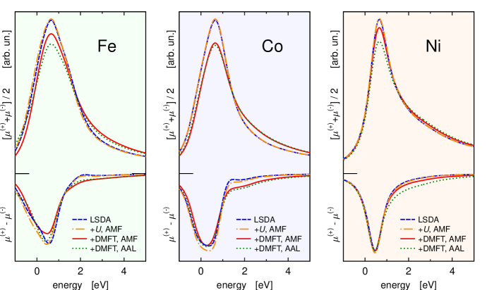
Figure 2: (Color online) $L_{3}$ edge XANES and XMCD spectra for Fe, Co, and Ni calculated on the basis of the plain LSDA, via the LSDA+$U$ with the AMF d.c. correction, via the LSDA+DMFT with the AMF d.c. correction and via the LSDA+DMFT with the AAL d.c. correction.

As it was mentioned in the introduction, in order to remedy many deficiencies of the LSDA as concerns the ground-state properties such as $\mu_{\mathrm{orb}}$ it is sufficient to include the correlations in a static way only, via the OP Brooks scheme or via the LSDA+$U$. However, these schemes do not bring any significant improvement concerning XAS. We demonstrate this by showing in Fig. 2 spectra calculated via the LSDA and via the LSDA+$U$ (the dashed and dash-dotted lines). Spectra obtained via the OP Brooks scheme are practically indistinguishable from the LSDA+$U$ results, so they are not shown here. Fig. 2 shows that the LSDA+$U$ method does not significantly alter the calculated spectra of transition metals with respect to the LSDA, similarly as it was found earlier for the OP Brooks scheme.Ebert (1996) This is in line with the concept that the OP Brooks scheme can be seen in fact as one of the limits of the more general LSDA+$U$ concept.Solovyev et al. (1998)

It was mentioned earlier in Sec. II that there are several ways to correct for the d.c. error in the LSDA+DMFT. Even though the AMF scheme seems to be the most reasonable d.c. procedure for 3$d$ TMs, one cannot a priori exclude the possibility that another d.c. scheme might be more appropriate for XAS. Therefore, we checked how the results change if the AAL d.c. scheme is employed instead of the AMF scheme. We found that the calculated spectra look quite similar (Fig. 2, dotted lines and full lines). A closer inspection of Fig. 2 reveals further that the calculated spectra split into two groups, according to whether the dynamic effects to the self-energy have been included (LSDA+DMFT calculations) or not (LSDA and LSDA+$U$ calculations). This is especially evident for the XANES spectra; e.g., in the case of Co, only two spectral curves can in fact be distinguished because the results are pairwise practically identical (upper part of the middle panel in Fig. 2). For the XMCD spectra, this splitting of the four spectra into two groups is clearly visible at the high-energy end of the Fe and Co $L_{3}$ peaks, between 1–3 eV in Fig. 2. The choice of the d.c. model has thus only a minor influence on the shapes of XANES and XMCD spectra. Nevertheless, it has some influence on the intensities of the peaks (see the following section).

IV.3 Relation to the $\mu_{\mathrm{orb}}^{(d)}/\mu_{\mathrm{spin}}^{(d)}$ ratio

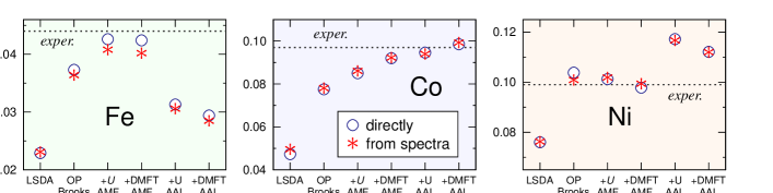
Figure 3: (Color online) The $\mu_{\mathrm{orb}}^{(d)}/\mu_{\mathrm{spin}}^{(d)}$ ratio evaluated directly and from theoretical XMCD spectra for calculations employing plain LSDA, OP Brooks, LSDA+$U$ with the AMF d.c. correction (denoted as “+$U$ AMF” on the horizontal axis), LSDA+DMFT with the AMF d.c. correction (“+DMFT AMF”), LSDA+$U$ with the AAL d.c. correction (“+$U$ AAL”) and LSDA+DMFT with the AAL d.c. correction (“+DMFT AAL”). The experimental ratios were taken those obtained from magneto-mechanical measurements.Reck and Fry (1969)

The changes in the XANES and XMCD spectra which result from the inclusion the $d$ band correlations are not very pronounced. One may ask to what degree are the changes significant at all: do they really reflect the different treatment of the correlations? The significance of the changes in the spectra can be assessed by comparing them with the changes of the ground-state properties. A suitable quantity in this respect is the $\mu_{\mathrm{orb}}/\mu_{\mathrm{spin}}$ ratio, as it is underestimated by the plain LSDA while it is correctly described by the LSDA+DMFT method. By applying the XMCD sum rules (5)–(6) to the theoretical spectrum, the ratio between the $d$ components of the magnetic moments, $\mu_{\mathrm{orb}}^{(d)}/\mu_{\mathrm{spin}}^{(d)}$, can be obtained and compared to the $\mu_{\mathrm{orb}}^{(d)}/\mu_{\mathrm{spin}}^{(d)}$ ratio obtained directly from the ground-state electronic structure. If this is done for different ways of accounting for the many body effects, the consistency of the changes in the spectra and in the ground-state properties can be monitored.

Our results are summarized in Fig. 3, where the $\mu_{\mathrm{orb}}^{(d)}/\mu_{\mathrm{spin}}^{(d)}$ ratio evaluated by the two ways mentioned above is shown for the plain LSDA, the OP Brooks scheme, the LSDA+$U$ and the LSDA+DMFT with the AMF d.c. correction and the LSDA+$U$ and the LSDA+DMFT with the AAL d.c. correction. The $\mu_{\mathrm{orb}}/\mu_{\mathrm{spin}}$ ratio derived from magneto-mechanical experiments is shown for comparison.Reck and Fry (1969) Use of $\mu_{\mathrm{orb}}/\mu_{\mathrm{spin}}$ instead of $\mu_{\mathrm{orb}}^{(d)}/\mu_{\mathrm{spin}}^{(d)}$ as an experimental reference is justified because both ratios differ by less then 5% and our focus is not on the agreement of $\mu_{\mathrm{orb}}$ with experiment ($\mu_{\mathrm{orb}}$ depends also on the value of $U$ anyway).Chadov et al. (2008)

It is obvious that the changes of the intensities of the $L_{3}$ and $L_{2}$ XMCD peaks reflect changes in $\mu_{\mathrm{orb}}/\mu_{\mathrm{spin}}$ via the sum rules very accurately. The differences between spectra calculated by different ways of dealing with the many body effects are thus relevant and consistent. Even relatively small changes in the intensities of XMCD peaks in Fig. 1 correspond to large changes in $\mu_{\mathrm{orb}}$, as can be seen in Tab. 1. The failure of the LSDA to reproduce the ratio of the $L_{3}$/$L_{2}$ XMCD peak intensities thus cannot be a simple consequence of the failure of the LSDA to yield correct orbital moments $\mu_{\mathrm{orb}}$.

IV.4 Effect of the core hole within the final state approximation

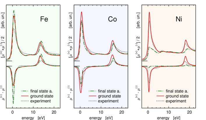
Figure 4: (Color online) L_2,3 edge XANES and XMCD spectra of Fe, Co, and Ni calculated within the LSDA+DMFT when the core hole is ignored (using the ground state potential) and when the core hole is included via the final state approximation. Experimental XANES and XMCD spectra are shown for comparison.

Accounting for the correlations in the $d$ band via the LSDA+DMFT improves the calculated spectra but the improvement is not dramatic (Fig. 1). A better agreement with experiment could presumably be obtained if the core hole was accounted for. This is quite a complicated task within the ab initio scheme. A technically relatively simple way of achieving this is via the “static” final state approximation (see Sec. II). For the $K$ edges, such a scheme sometimes improves the XANES (e.g., for the Zn edge in ZnSeŠipr et al. (1997) or for the Si edge in quartz)Wu et al. (1998) while sometimes it has only a minor effect (early transition metals).Zeller (1988) However, the final state approximation need not work for the L_2,3 edges which involve transitions to semi-localized $d$ states: by promoting a 2$p$ electron into the valence states one may effectively fill the $d$ band of the photoabsorbing atom, suppressing to a large extent the intensity of the white line. This issue will be explored in the following.

To see the effect of the final state approximation, we applied it on top of the LSDA+DMFT procedure. The results are shown in Fig. 4. It is evident that this procedure does not generally improve the L_2,3 edge spectra of late 3$d$ TMs. Hardly any systematic trend in the effect of the core hole can be found — neither as concerns the shape of the white lines, nor as concerns the ratio of the intensities of the $L_{3}$ and $L_{2}$ peaks. For Fe, we observe an increase of the ratio of intensities of the $L_{3}$ and $L_{2}$ XMCD peaks, in agreement with experiment. For Co, the final state approximation produces only minor changes with respect to the ground state calculations. For Ni, however, including the core hole via the final state approximation substantially worsens the agreement with experiment — the XAS white lines as well as the prominent XMCD peaks practically disappear! A similar situation occurs if the final state approximation is applied over the plain LSDA (therefore, only the LSDA+DMFT results are shown here).

We tested this scheme also by using a half-filled core hole, i.e., employing the Slater transition state method. Sometimes this procedure works well for the $K$ edge spectra.Mizoguchi et al. (2000); Leetmaa et al. (2010) Satisfying results were also reported for the Cu $L_{3}$ edge XANES.Luitz et al. (2001) In our case, however, the Slater transition state method does not bring any substantial improvement — the results just lie approximately half-way between the results obtained without a core hole and with a full core hole, so they are not shown here.

Our results demonstrate that the final state approximation is unsuitable for describing the L_2,3 edge XAS in late 3$d$ TMs. This applies for calculations based on the plain LSDA as well as on the LSDA+DMFT method.

V Conclusions

Our goal was to find out whether the differences commonly occurring between the experimental L_2,3 edge XANES and XMCD spectra of 3$d$ transition metals on the one hand and ab-initio calculations on the other hand are mainly due to the way the LSDA deals with the correlations. By performing the LSDA+DMFT calculations, we found that if valence- and conduction-band correlations are included, the spectra change in the right direction with respect to the plain LSDA. In particular, the LSDA+DMFT yields asymmetric $L_{3}$ XAS white lines. The improvement is, however, rather incremental than dramatic. The ratio of the intensities of the $L_{3}$ and $L_{2}$ XAS and XMCD peaks is not significantly improved by the LSDA+DMFT formalism. The changes in the intensities of the XMCD peaks are, nevertheless, consistent with the changes of the $\mu_{\mathrm{orb}}/\mu_{\mathrm{spin}}$ ratio as suggested by the XMCD sum rules.

When the core hole is additionally accounted for within the final state approximation, the agreement between theory and experiment generally does not improve (in the case of Ni, it substantially worsens). It appears, therefore, that to get a decisive improvement of ab-initio calculations of the L_2,3 edge XAS and XMCD spectra of 3$d$ metals, the dynamic correlations between the excited photoelectron and the core hole have to be taken into account.