Comparison of charged particle energy loss in epitaxial with free-standing multilayer graphene.

Abstract

We present a formalism and numerical results for the energy loss of a charged particle scattered at an arbitrary angle from epitaxially grown multilayer graphene (MLG). It is compared with that of free-standing graphene layers. Specifically, we investigated the effect of the substrate induced energy gap on one of the layers. The gap yields collective plasma oscillations whose characteristics are qualitatively and quantitatively different from those produced by Dirac fermions in gapless graphene. The range of wave numbers for undamped self-sustaining plasmons is increased as the gap is increased, thereby increasing and red-shifting the MLG stopping power for some range of charged particle velocity. We also applied our formalism to interpret several distinct features of experimentally obtained electron energy loss spectroscopy (EELS) data.

I Introduction

Electron energy loss spectroscopy (EELS) has been considered for many systems dating back to the classic paper of Ritchie ritchie on surface plasmons for a slab of dielectric material in the local limit and subsequently generalized to a non-local dielectric function by Gumbs and Horing. slab The non-locality was included in Ref. slab, through the screening of the electron-electron interaction produced by single-particle excitations and plasmon modes. Fessatidis, et al. fessatidis recently adopted the formalism of Horing, et al. tso for a two-dimensional electron gas (2DEG) and Gumbs and Balassis GG for a nanotube to graphene with the aid of the polarization function calculated by Wunsch, et al. wunsch for conventional Dirac electrons.

There have been several recent papers which considered the effects which a circularly polarized electromagnetic field (CPEF), kibis ; roslyak spin-orbit interaction (SOI) SOI in suspended graphene or the sublattice symmetry breaking (SSB) by an underlying polar substrate SOI-2 ; li_2009 ; giovannetti_2007 in epitaxial graphene may have on the energy band structure and plasma excitations roslyak of a graphene sheet. Under these conditions, there is a gap between the valence and conduction bands as well as between the intra-band and inter-band electron-hole continuum of the otherwise semimetallic Dirac system. wunsch ; shung1 ; shung2 Additionally, the interplay between the single-particle excitations in the long wavelength limit results in dielectric screening of the Coulomb interaction which produces an undamped plasmon mode that appears in the gap separating the two types of electron-hole modes forming a continuum. By this we mean that a self-sustained collective plasma mode is not supported by exciting either the intra-band or inter-band single-particle modes only. Furthermore, since the Dirac electrons now acquire a non-zero effective mass, one can produce a long wavelength plasmon mode as in the 2DEG by intra-band excitations only. These properties of the plasma modes give rise to noticeable differences in the behavior of the stopping power of gapped graphene compared with conventional free-standing exfoliated multilayer graphene.

Multi-layer epitaxially grown graphene (MLG) may become a valuable and relatively cheap alternative to rather expensive exfoliated graphene. Recent angle-resolved photoemission spectroscopy (ARPES) experiments unambiguously demonstrated almost perfect Dirac cones on most of the layers. That is the electrons in the layers behave as if the layers are uncoupled in contrast to Bernal stacking in bi-layer graphene. SPRINKLE:2010 Although some layers may establish bi-layer structures the interaction between the first and the buffer layer (the one sitting on top of the SiC substrate) is always weak. MATTAUSCH:2007 ; MALLET:2007 The spectral function of MLG on SiC substrate suggests the energy gap of few hundreds of meV. However the exact gap opening mechanism in epitaxial graphene is still under debate. rotenberg_2008 The complexity comes from the fact that the graphene sample sits on top of a buffer layer which provides an additional mid gap level, thus obscuring the exact energy dispersion curve and requires numerical ab initio calculations. kim_2008 In addition, the DOS around Fermi energy failed to indicate the gap. SPRINKLE:2010 This ambiguity stimulated discussion regarding the symmetry breaking gap zhou_2007 versus the effects due to electron-electron interaction. bostwik_2007 This also indicates the importance of alternative techniques capable of identifying the induced gap by a buffer layer on a substrate.

EELS may be employed to ascertain the plasmon frequencies in single and double layer graphene. The Raman shift of the scattered electrons provides both particle-hole and plasmon excitation frequencies, which are usually characterized by their spectral weight, a quantity that depends on the transferred energy $\hbar\omega$ and in-plane momentum $\hbar q$. This allows mapping of the plasmon dispersions $\omega_{p}(q)$. LU:2009 Here we calculate EELS spectra in order to pinpoint the effect of the substrate induced gap in MLG.

The outline of the remainder of this paper is as follows. In Sec. II, we derive the energy loss for charged particles incident on multiple electron layers at an arbitrary angle of incidence. In Sec. III, this formalism is applied to MLG with a gapped buffer layer. Our numerical simulations are compared with experimental results of Lu and Loh LU:2009 in Sec. IV. A summary is presented in Sec. V.

II Energy Loss Formalism

We shall consider an inhomogeneous medium (in the $\hat{\mathbf{z}}$ direction) described by a nonlocal dielectric function $\epsilon\left({1;2}\right)$. Here, we have introduced space-time points, such as $i=\left({z_{i},\mathbf{r}_{i},t_{i}}\right)$, where the $z$ spacial coordinate has been separated out due to the inhomogeneity and making cylindrical coordinates suitable for our discussion. Our focus is the calculation of energy loss of a charged particle $Ze$ moving along a prescribed trajectory $z_{1}+\mathbf{v}t_{1}$. Due to non-locality of the dielectric function, the charged particle experiences a frictional force given by the gradient of the effective potential as

$$\mathbf{F}(1)=-Ze\left[{\nabla_{1}\Phi_{\texttt{tot}}(1)}\right]_{1=z_{1}+\mathbf{v}t_{1}}\ .$$ (1)

The total potential can be determined from the following system of equations

$$\Phi_{\texttt{tot}}(1)=\int d^{4}2\ \epsilon^{-1}(1;2)\Phi_{\texttt{ext}}(2)\ ,$$ (2)

$$\nabla^{2}_{1}\Phi_{\texttt{ext}}(1)=-\frac{Ze}{\epsilon_{0}}\,\delta(1-z_{1}-\mathbf{v}t_{1})\ .$$ (3)

Solving Eq. (3) by Fourier transformation and substituting the result into Eq. (2) and then into (1), we obtain the components of the frictional force as

$$\mathbf{F}_{\parallel}(1)=-\frac{\left({Ze}\right)^{2}}{\left({2\pi}\right)^{3}\epsilon_{0}}\int\limits_{-\infty}^{\infty}dz_{2}\int i\mathbf{q_{\parallel}}\,d^{2}\ \mathbf{q_{\parallel}}\int\limits_{-\infty}^{\infty}dq_{z}\,\texttt{e}^{iq_{z}\left({z_{2}-z_{1}-v_{z}t_{1}}\right)}\,q^{-2}\epsilon^{-1}\left({z_{1}+v_{z}t_{1},z_{2};q_{\parallel},\mathbf{q}\cdot\mathbf{v}}\right)\ ,$$ (4)

$$\mathbf{F}_{\perp}(1)=-\frac{\left({Ze}\right)^{2}}{\left({2\pi}\right)^{3}\epsilon_{0}}\int\limits_{-\infty}^{\infty}dz_{2}\int d^{2}\mathbf{q_{\parallel}}\int\limits_{-\infty}^{\infty}dq_{z}\texttt{e}^{iq_{z}\left({z_{2}-z_{1}-v_{z}t_{1}}\right)}\,q^{-2}\frac{\partial}{\partial\left({z_{1}+v_{z}t_{1}}\right)}\,\epsilon^{-1}\left({z_{1}+v_{z}t_{1},z_{2};q_{\parallel},\mathbf{q}\cdot\mathbf{v}}\right)\ .$$ (5)

We assume that the particle trajectory begins at $t=-\infty$ and ends at $t=\infty$ with its motion in vacuum. The net energy lost due to the frictional force between it and the plasma during this motion may be expressed as

$$W=\int\limits_{-\infty}^{\infty}dt_{1}\,\mathbf{v}(t_{1})\cdot\mathbf{F}(1)\ .$$ (6)

It is convenient to partition the loss as $W=W_{\parallel}+W_{\perp}$. The energy loss due to parallel and perpendicular motions may be written as

$$W_{\parallel}\left({z_{1},\mathbf{v}}\right)=-\frac{i\left({Ze}\right)^{2}}{\left({2\pi}\right)^{3}\epsilon_{0}}\int\limits_{-\infty}^{\infty}dt_{1}\int\limits_{-\infty}^{\infty}dz_{2}\int d^{2}\mathbf{q_{\parallel}}\ \left({\mathbf{q_{\parallel}}\cdot\mathbf{v}_{\parallel}}\right)\int\limits_{-\infty}^{\infty}dq_{z}\ \texttt{e}^{iq_{z}\left({z_{2}-z_{1}-v_{z}t_{1}}\right)}\,q^{-2}\epsilon^{-1}\left({z_{1}+v_{z}t_{1},z_{2};q_{\parallel},\mathbf{q}\cdot\mathbf{v}}\right)\ ,$$ (7)

$$W_{\perp}\left({\mathbf{v}}\right)=-\frac{i\left({Ze}\right)^{2}}{\left({2\pi}\right)^{3}\epsilon_{0}}\int\limits_{-\infty}^{\infty}dz_{1}\int\limits_{-\infty}^{\infty}dz_{2}\int d^{2}\mathbf{q_{\parallel}}\int\limits_{-\infty}^{\infty}dq_{z}\ q_{z}\texttt{e}^{iq_{z}\left({z_{2}-z_{1}}\right)}\,q^{-2}\epsilon^{-1}\left({z_{1},z_{2};q_{\parallel},\mathbf{q}\cdot\mathbf{v}}\right)\ .$$ (8)

In Eq. (8), integration by parts was carried out, along with the condition that the charged particle starts and ends in vacuum: $\epsilon^{-1}\left({-\infty,z_{2};q_{\parallel},\mathbf{q}\cdot\mathbf{v}}\right)=\epsilon^{-1}\left({\infty,z_{2};q_{\parallel},\mathbf{q}\cdot\mathbf{v}}\right)=1$. The above general expressions can be simplified further, for the practically important cases of parallel, perpendicular and traversing motion.

II.1 Charged Particle moving parallel to the surface ($\mathbf{v}_{z}=0$)

First, we assume that the charged particle travels parallel to the $x,y$ plane with velocity component $v_{z}=0$. In this case, to simplify Eq. (7), we can use the following identities:

$$\int\limits_{-\infty}^{\infty}dq_{z}\ q^{-2}\texttt{e}^{iq_{z}\left({z_{2}-z_{1}}\right)}=2\pi\frac{\texttt{e}^{-q_{\parallel}|{z_{1}-z_{2}}|}}{2q_{\parallel}}\ ,$$ (9)

$$i\int\left({\mathbf{q_{\parallel}}\cdot\mathbf{v}_{\parallel}}\right)d^{2}\mathbf{q_{\parallel}}\epsilon^{-1}\left({z_{1},z_{2};q_{\parallel},\mathbf{q_{\parallel}}\cdot\mathbf{v_{\parallel}}}\right)=-2i\int\limits_{0}^{\infty}v_{\parallel}dq_{\parallel}\ q^{2}_{\parallel}\int\limits_{-1}^{1}\frac{\cos\theta\ d(\cos\theta)}{\sqrt{1-\cos^{2}\theta}}\epsilon^{-1}\left({z_{1},z_{2};q_{\parallel},q_{\parallel}v_{\parallel}\cos\theta}\right)$$ (10)

$$=-\int d^{2}\mathbf{q_{\parallel}}\ \left({\mathbf{q_{\parallel}}\cdot\mathbf{v}_{\parallel}}\right)\Im\texttt{m}\epsilon^{-1}\left({z_{1},z_{2};q_{\parallel},\mathbf{q_{\parallel}}\cdot\mathbf{v_{\parallel}}}\right)\ .$$

In the above Eq. (10), to integrate over the angle we used the parity of the inverse dielectric function, i.e.,

$$\epsilon^{-1}\left({z_{1},z_{2};-\mathbf{q}_{\parallel},-\omega}\right)=\left[\epsilon^{-1}\left({z_{1},z_{2};\mathbf{q}_{\parallel},\omega}\right)\right]^{\ast}\ .$$ (11)

Consequently, we obtain the energy loss in the parallel case as

$$W_{\parallel}\left({z_{1},v_{\parallel}}\right)=\left({\frac{Ze}{2\pi}}\right)^{2}\int\limits_{-\infty}^{\infty}dt_{1}\int\limits_{-\infty}^{\infty}dz_{2}\int d^{2}\mathbf{q_{\parallel}}\ \left({\mathbf{q_{\parallel}}\cdot\mathbf{v}_{\parallel}}\right)\frac{\texttt{e}^{-q_{\parallel}|{z_{1}-z_{2}}|}}{2\epsilon_{0}q_{\parallel}}\Im\texttt{m}\epsilon^{-1}\left({z_{1},z_{2};q_{\parallel},\mathbf{q_{\parallel}}\cdot\mathbf{v_{\parallel}}}\right)\ .$$ (12)

Since the integrand in the above expression does not depend on time, it is more convenient to represent it in the form of constant energy loss rate (per unit time) as

$$W_{\parallel}\left({z_{1},v_{\parallel}}\right)=\int\limits_{-\infty}^{\infty}dt_{1}\frac{dW_{\parallel}}{dt}$$ (13)

$$\frac{dW_{\parallel}}{dt}\left({z_{1},v_{\parallel}}\right)=-\left({\frac{Ze}{2\pi}}\right)^{2}\int\limits_{-\infty}^{\infty}dz_{2}\int d^{2}\mathbf{q_{\parallel}}\ \left({\mathbf{q_{\parallel}}\cdot\mathbf{v}_{\parallel}}\right)\frac{\texttt{e}^{-q_{\parallel}|{z_{1}-z_{2}}|}}{2\epsilon_{0}q_{\parallel}}\Im\texttt{m}\epsilon^{-1}\left({z_{1},z_{2};q_{\parallel},-\mathbf{q_{\parallel}}\cdot\mathbf{v_{\parallel}}}\right)\ .$$

In the above, we used the odd parity of the imaginary part of the inverse dielectric function. The rate of the energy loss expressed per unit length is usually referred to as the stopping power $S=\frac{dW_{\parallel}}{v_{\parallel}dt}$.

II.2 Charged Particle moving perpendicular to the surface ($\mathbf{v}_{\parallel}=0$)

Now, let us assume that the particle has only velocity component perpendicular to the $x,y$ plane, i.e., $v_{\parallel}=0$. We shall focus on the last integration in Eq. (8), by changing the variable $\omega=q_{z}v_{z}$, so that we can perform the series string of simplifications on it, namely,

$$\frac{1}{v_{z}^{2}}\int\limits_{-\infty}^{\infty}d\omega\ \omega\frac{\texttt{e}^{i\omega\left({z_{2}-z_{1}}\right)/v_{z}}}{q_{\parallel}^{2}+\left({\omega/v_{z}}\right)^{2}}\epsilon^{-1}\left({z_{1},z_{2};q_{\parallel},\omega}\right)$$ (14)

$$=\frac{1}{v_{z}^{2}}\int\limits_{0}^{\infty}d\omega\ \omega\frac{\texttt{e}^{i\omega\left({z_{2}-z_{1}}\right)/v_{z}}}{q_{\parallel}^{2}+\left({\omega/v_{z}}\right)^{2}}\epsilon^{-1}\left({z_{1},z_{2};q_{\parallel},\omega}\right)-\frac{1}{v_{z}^{2}}\int\limits_{0}^{\infty}d\omega\ \omega\frac{\texttt{e}^{-i\omega\left({z_{2}-z_{1}}\right)/v_{z}}}{q_{\parallel}^{2}+\left({\omega/v_{z}}\right)^{2}}(\epsilon^{\star})^{-1}\left({z_{1},z_{2};q_{\parallel},\omega}\right)$$

$$=\frac{2i}{v_{z}^{2}}\int\limits_{0}^{\infty}\frac{d\omega\ \omega}{q_{\parallel}^{2}+\left({\omega/v_{z}}\right)^{2}}\Im\texttt{m}\;\texttt{e}^{i\omega\left({z_{2}-z_{1}}\right)/v_{z}}\epsilon^{-1}\left({z_{1},z_{2};q_{\parallel},\omega}\right)\ .$$

Consequently, by combining Eqs. (14) and (8), we obtain the following energy loss in the perpendicular case as

$$W_{\perp}\left({v_{z}}\right)=\frac{2\left({Ze}\right)^{2}}{\left({2\pi}\right)^{3}\epsilon_{0}}\Im\texttt{m}\;\int\limits_{-\infty}^{\infty}dz_{1}\int\limits_{-\infty}^{\infty}dz_{2}\int d^{2}\mathbf{q}_{\parallel}\int\limits_{0}^{\infty}\frac{d\omega\ \omega}{\left({q_{\parallel}v_{z}}\right)^{2}+\omega^{2}}\epsilon^{-1}\left({z_{1},z_{2};q_{\parallel},\omega}\right)\texttt{e}^{i\omega\left({z_{2}-z_{1}}\right)/v_{z}}\ .$$ (15)

Now, let us apply the energy loss formalism to single and double layers of of epitaxially grown graphene. The epitaxial form of graphene usually features the energy gap, which may be controlled by an external electric field from a gate.

II.3 Charged Particle traversing/reflected from the graphene layers at an arbitrary angle

For the case when the charged particle crosses the layers, none of the components of the velocity is zero. As in the perpendicular case, the initial position of the particle is of little importance and we may change variable $z_{1}+v_{z}t\to z_{1}$ in Eq. (7), followed by adding the obtained equation to Eq. (8), giving

$$W_{\theta}\left({\mathbf{v}}\right)=-\frac{i\left({Ze}\right)^{2}}{\left({2\pi}\right)^{3}v_{z}\epsilon_{0}}\int\limits_{-\infty}^{\infty}dz_{1}\,\int\limits_{-\infty}^{\infty}dz_{2}\,\int\limits_{-\infty}^{\infty}dq_{z}\int d^{2}\,\mathbf{q}_{\parallel}\texttt{e}^{iq_{z}\left({z_{2}-z_{1}}\right)}\epsilon^{-1}\left({z_{1},z_{2};q_{\parallel},\mathbf{q}\cdot\mathbf{v}}\right)q^{-2}\mathbf{q}\cdot\mathbf{v}$$ (16)

$$=\frac{2\left({Ze}\right)^{2}}{\left({2\pi}\right)^{3}v_{z}\epsilon_{0}}\Im\texttt{m}\;\int\limits_{-\infty}^{\infty}dz_{1}\,\int\limits_{-\infty}^{\infty}dz_{2}\,\int\limits_{0}^{\infty}dq_{z}\,\int d^{2}\mathbf{q}_{\parallel}\,\texttt{e}^{iq_{z}\left({z_{2}-z_{1}}\right)}\epsilon^{-1}\left({z_{1},z_{2};q_{\parallel},\mathbf{q}\cdot\mathbf{v}}\right)q^{-2}\mathbf{q}\cdot\mathbf{v}\ .$$

The last expression is obtained by changing the sign $\mathbf{q}\to-\mathbf{q}$ and utilizing the symmetry relation Eq. (11). We now rewrite the energy loss via the energy-loss probability spectral function $\mathcal{P}\left({\omega}\right)$. To do so, we introduce $\omega=\mathbf{q}\cdot\mathbf{v}=q_{z}v_{z}+\mathbf{q}_{\parallel}\cdot\mathbf{v}_{\parallel}$, thereby obtaining

$$W_{\theta}\left({\mathbf{v}}\right)=\int\limits_{0}^{\infty}d\omega\ \omega\mathcal{P}\left({\omega,\mathbf{v}}\right)$$ (17)

$$\mathcal{P}\left({\omega,\mathbf{v}}\right)=\frac{2(Ze)^{2}}{\left({2\pi}\right)^{3}\epsilon_{0}}\Im\texttt{m}\int\limits_{-\infty}^{\infty}dz_{1}\int\limits_{-\infty}^{\infty}dz_{2}\int d^{2}\mathbf{q}_{\parallel}\ \epsilon^{-1}\left({z_{1},z_{2};\mathbf{q}_{\parallel},\omega}\right)\frac{\exp\left({i\left({\omega-\mathbf{q}_{\parallel}\cdot\mathbf{v}_{\parallel}}\right)(z_{2}-z_{1})/v_{z}}\right)}{\left({q_{\parallel}v_{z}}\right)^{2}+\left({\omega-\mathbf{q}_{\parallel}}\cdot\mathbf{v}_{\parallel}\right)^{2}}\ .$$

An alternative derivation of the above equation is provided in Appendix A. One may show in a straightforward way that the above general expression may be expressed as Eq. (15) in the case of $\mathbf{v}_{\parallel}=0$. The other limiting case Eq. (13) is less trivial. It is obtained from Eq. (17) by taking the following limits $\lim\limits_{v_{z}\rightarrow 0}\left({\omega-\mathbf{q}_{\parallel}\cdot\mathbf{v}_{\parallel}}\right)/v_{z}=q_{z}$, $\lim\limits_{v_{z}\rightarrow 0}dz_{1}/v_{z}=dt_{1}$ and using Eq. (9).

It is straightforward to derive the energy loss when the charged particle is elastically reflected from the Si surface (at $z_{1}=0$) of the SiC substrate, yielding

$$\mathcal{P}\left({\omega,\mathbf{v}}\right)=\frac{4(Ze)^{2}}{\left({2\pi}\right)^{3}\epsilon_{0}}\Im\texttt{m}\int\limits_{-\infty}^{\infty}dz_{1}\int\limits_{-\infty}^{\infty}dz_{2}\int d^{2}\mathbf{q}_{\parallel}\ \epsilon^{-1}\left({z_{1},z_{2};\mathbf{q}_{\parallel},\omega}\right)\frac{\cos\left({\left({\omega-\mathbf{q}_{\parallel}\cdot\mathbf{v}_{\parallel}}\right)(z_{2}-z_{1})/v_{z}}\right)}{\left({q_{\parallel}v_{z}}\right)^{2}+\left({\omega-\mathbf{q}_{\parallel}}\cdot\mathbf{v}_{\parallel}\right)^{2}}\ .$$ (18)

For multiple graphene layers separated by distance $d$, we can assume wave function localization on the layers, and neglect their overlap. Therefore, we obtain Kushwaha-2001 ; EELS_SSC

$$\epsilon^{-1}\left({z_{1},z_{2};q_{\parallel},\omega)}\right)=\delta\left({z_{1}-z_{2}}\right)+\sum\limits_{j,j^{\prime}}v_{q}\texttt{e}^{-q_{\parallel}|{z_{1}-jd}|}\Pi^{(0)}_{j}\left({\delta_{j,j^{\prime}}-\Pi^{(0)}_{j}v_{q}\texttt{e}^{-q_{\parallel}|{j-j^{\prime}}|d}}\right)^{-1}\delta\left({z_{2}-j^{\prime}d}\right)\ ,$$ (19)

where the 2D Fourier transform of the Coulomb interaction has been introduced by $v_{q}=2\pi e^{2}/\epsilon_{s}q_{\parallel}$ with $\epsilon_{s}=4\pi\epsilon_{0}\epsilon_{b}$ for background dielectric constant $\epsilon_{b}$. The arguments $\left({q_{\parallel},\omega}\right)$ of the noninteracting polarization function $\Pi^{(0)}_{j}$ on the $j^{\text{th}}$ layer have been omitted. Equation (19) can be substituted into Eq. (17) and, after calculating the integrals over $z_{1}$ and $z_{2}$, we obtain:

$$\left[\begin{array}[]{c}\mathcal{P}_{\mathcal{T}}\left({\omega,\,\mathbf{v}}\right)\\ \mathcal{P}_{\mathcal{R}}\left({\omega,\,\mathbf{v}}\right)\end{array}\right]=\frac{4(Ze)^{2}}{\left({2\pi}\right)^{3}\epsilon_{0}}\Im\texttt{m}\sum\limits_{j,j^{\prime}}\int d^{2}\mathbf{q}_{\parallel}\ \frac{v_{z}^{2}\,v_{q}\,\Pi_{j,j^{\prime}}}{\left[{\left({q_{\parallel}v_{z}}\right)^{2}+\left({\omega-\mathbf{q}_{\parallel}}\cdot\mathbf{v}_{\parallel}\right)^{2}}\right]^{2}}\left[\begin{array}[]{c}\mathcal{T}\\ \mathcal{R}\end{array}\right]\ .$$ (24)

Additionally, we have introduced auxiliary expressions for reflective $\mathcal{R}$ and transmissive $\mathcal{T}$ particle trajectories:

$$\mathcal{T} = q_{\parallel}\exp\left[{-iq_{z}(j-j^{\prime})d}\right]\ ,$$ (25)

$$\mathcal{R} = 2q_{\parallel}\cos\left[{q_{z}(j-j^{\prime})d}\right]+\texttt{e}^{-q_{\parallel}jd}\left[{q_{z}\texttt{sin}(q_{z}j^{\prime}d)-q_{\parallel}\cos(q_{z}j^{\prime}d)}\right]\ ,$$ (26)

as well as the random-phase approximation (RPA) polarization matrix elements:

$$\Pi_{j,j^{\prime}}=\Pi_{j^{\prime}}^{(0)}\left({\delta_{j,j^{\prime}}-v_{q}\,\Pi^{(0)}_{j}\,\texttt{e}^{-q_{\parallel}|{j-j^{\prime}}|d}}\right)^{-1}\ .$$ (27)

For either a single (upper) or double (lower) layer configuration, Eq. (24) assumes the form

$$\mathcal{P}_{\mathcal{T}(\mathcal{R})}\left({\omega,\,\mathbf{v}}\right)=\frac{4(Ze)^{2}}{\left({2\pi}\right)^{3}\epsilon_{0}}\Im\texttt{m}\int\frac{v_{z}^{2}\,d^{2}\mathbf{q}_{\parallel}}{\left[{\left({q_{\parallel}v_{z}}\right)^{2}+\left({\omega-\mathbf{q}_{\parallel}}\cdot\mathbf{v}_{\parallel}\right)^{2}}\right]^{2}}$$

$$\times\left\{\begin{array}[]{c}q_{\parallel}\,v_{q}\Pi^{(0)}_{1}\left[1-v_{q}\Pi^{(0)}_{1}\right]^{-1}\\ \\ \mathcal{T}(\mathcal{R})\left[\left({1-v_{q}\Pi^{(0)}_{1}}\right)\left({1-v_{q}\Pi^{(0)}_{2}}\right)-v^{2}_{q}\,\Pi^{(0)}_{1}\Pi^{(0)}_{2}\,\texttt{e}^{-2q_{\parallel}d}\right]^{-1}\end{array}\right.\ .$$ (28)

Here, we have redefined the transmitted (reflected) notations as

$$\mathcal{T}=2q_{\parallel}\,v^{2}_{q}\,\texttt{e}^{-q_{\parallel}d}\,\cos(q_{z}d)\,\Pi^{(0)}_{1}\Pi^{(0)}_{2}+v_{q}\left({\Pi^{(0)}_{1}+\Pi^{(0)}_{2}-2v_{q}\,\Pi^{(0)}_{1}\Pi^{(0)}_{2}}\right)\ ,$$ (29)

$$\mathcal{R}=\texttt{e}^{-3q_{\parallel}d}\,v_{q}\left(\Pi^{(0)}_{2}\,\texttt{e}^{q_{\parallel}d}\,\left[2q_{\parallel}\,\texttt{e}^{2q_{\parallel}d}+q_{z}\,\texttt{sin}(2q_{z}d)-q_{\parallel}\,\cos(2q_{z}d)\right]\right.$$ (30)

$$+\Pi^{(0)}_{1}\left\{v_{q}\,\Pi^{(0)}_{2}\left[q_{z}\left(1-\texttt{e}^{2q_{\parallel}d}\right)\texttt{sin}(q_{z}d)+q_{\parallel}\left({5\texttt{e}^{2q_{\parallel}d}-1}\right)\cos(q_{z}d)-4q_{\parallel}\,\texttt{e}^{3q_{\parallel}d}\right]\right.$$

$$\left.\left.+\texttt{e}^{2q_{\parallel}d}\left[2q_{\parallel}\,\texttt{e}^{q_{\parallel}d}+q_{z}\,\texttt{sin}(q_{z}d)-q_{\parallel}\,\cos(q_{z}d)\right]\right\}\right)\ .$$

III Energy loss in MLG

Let us consider MLG with the $SiC(0001)$ substrate lying in the $z=0$ plane. We shall ignore contribution to EELS from $\sigma-$electrons, substrate surface imperfections and its optical (FK-) phonons LIU:2010 as well as the resonant plasmon coupling with single-particle excitations. TEGENKAMP:2011 For simplicity, we shall limit ourselves to only one or two graphene layers located at $z=d$ and $z=2d$. In accordance with the classification in Ref. LU:2009, those are referred to as 0ML and 1ML correspondingly. One of the effects of the substrate is $n-$doping of the graphene layers, thus causing the chemical potential $\mu_{i}>0$, where $i=0,1$ labels the layers. Hereafter we presume that both layers are held at the same chemical potential $\mu$. The chemical potential $\mu$ is related to the Fermi wave vector $k_{F}=\mu/\hbar v_{F}$. The other effect is more subtle, and affects only zero layer. This layer, often referred to as a ”buffer layer”, exhibits crossover from Dirac to conventional 2DEG by virtue of the substrate induced gap $E_{g}$. Ultimately, this gap is related to the symmetry breaking between $A$ and $B$ sublattices of the buffer graphene layer. This effect depends on two main factors, namely, the angle between the $\Gamma-K$ line and the principal axis of the SiC substrate and the degree of the hydrogen passivation of the substrate. Formally, the $\pi-$electron dispersion around the $K\ (K^{\prime})$ point becomes

$$E_{k}=\sqrt{\left({\hbar v_{F}k}\right)^{2}+\left({E_{g}/2}\right)^{2}}\ ,$$ (31)

where $v_{F}$ is the Fermi velocity for free standing graphene. The effect of the substrate on the other graphene layers is mitigated by the buffer layer and the electrons obey conventional Dirac dispersion ($E_{g}=0$ in Eq. (31)). Since it plays a crucial role in EELS (28), we give the full form of noninteracting polarization along the real frequency axis:

$$\Pi^{(0)}_{j}(q,\omega+i0^{+})=-\frac{2\mu}{\pi\hbar^{2}v^{2}_{F}}+\frac{q^{2}}{4\pi\sqrt{|{\hbar^{2}v_{F}^{2}q^{2}-\hbar^{2}\omega^{2}}|}}$$ (32)

$$\times\left\{\left[iG_{>}(x_{1,-})-iG_{>}(x_{1,+})\right]1_{<}+\left[G_{<}(x_{1,-})+iG_{>}(x_{1,+})\right]2_{<}\right.$$

$$+\left[G_{<}(x_{1,+})+G_{<}(x_{1,-})\right]3_{<}+\left[G_{<}(x_{1,-})-G_{<}(x_{1,+})\right]4_{<}+\left[G_{>}(x_{1,+})-G_{>}(x_{1,-})\right]1_{>}$$

$$+\left[G_{>}(x_{1,+})+iG_{<}(x_{1,-})\right]2_{>}+\left[G_{>}(x_{1,+})-G_{>}(-x_{1,-})-i\pi(2-x_{0}^{2})\right]3_{>}$$

$$+\left.\left[G_{>}(-x_{1,-})+G_{>}(x_{1,+})-i\pi(2-x_{0}^{2})\right]4_{>}+\left[G_{0}(x_{1,+})-G_{0}(x_{1,-})\right]5_{>}\right\}\ .$$

Here, the following notations for the region functions have been introduced:

$$x_{0} = \sqrt{1+\frac{E_{g}^{2}}{\hbar^{2}v_{F}^{2}q^{2}-\hbar^{2}\omega^{2}}}\ ,$$

$$x_{1,\pm} = \frac{2\mu\pm\hbar\omega}{\hbar v_{F}q}\ ,$$

$$x_{2,\pm} = \sqrt{\hbar^{2}v_{F}^{2}(q\pm k_{F})^{2}+(E_{g}/2)^{2}}\ ,$$

$$x_{3} = \sqrt{\hbar^{2}v^{2}_{F}q^{2}+E^{2}_{g}}\ ,$$

$$G_{<}(x) = x\sqrt{x_{0}^{2}-x^{2}}-(2-x_{0}^{2})\cos^{-1}(x/x_{0})\ ,$$

$$G_{>}(x) = x\sqrt{x^{2}-x_{0}^{2}}-(2-x_{0}^{2})\cosh^{-1}(x/x_{0})\ ,$$

$$G_{0}(x) = x\sqrt{x^{2}-x_{0}^{2}}-(2-x_{0}^{2})\sinh^{-1}(x/\sqrt{-x_{0}^{2}})\ ,$$

with the corresponding regions defined as

$$1_{<}= \theta\left({\mu-x_{2,-}-\hbar\omega}\right)\ ,$$

$$2_{<}= \theta\left({-\hbar\omega-\mu+x_{2,-}}\right)\theta\left({\hbar\omega+\mu-x_{2,-}}\right)\theta\left({\mu+x_{2,+}-\hbar\omega}\right)\ ,$$

$$3_{<}= \theta\left({-\mu+x_{2,-}-\hbar\omega}\right)\ ,$$

$$4_{<}= \theta\left({\hbar\omega+\mu-x_{2,+}}\right)\theta\left({\hbar v_{F}q-\hbar\omega}\right)\ ,$$

$$1_{>}= \theta\left({2k_{F}-q}\right)\theta\left({\hbar\omega-x_{3}}\right)\theta\left({\mu+x_{2,-}-\hbar\omega}\right)\ ,$$

$$2_{>}= \theta\left({\hbar\omega-\mu-x_{2,-}}\right)\theta\left({\mu+x_{2,+}-\hbar\omega}\right)\ ,$$

$$3_{>}= \theta\left({\hbar\omega-\mu-x_{2,+}}\right)$$

$$4_{>}= \theta\left({q-2k_{F}}\right)\theta\left({\hbar\omega-x_{3}}\right)\theta\left({\mu+x_{2,-}-\hbar\omega}\right)\ ,$$

$$5_{>}= \theta\left({\hbar\omega-\hbar v_{F}q}\right)\theta\left({x_{3}-\hbar\omega}\right)\ .$$

Given Eq. (32), the plasmon dispersion relation can be obtained as zeros of the real part of Eq. (19). Alternatively, those solutions are given by the poles of the imaginary part of the RPA polarization in Eq. (27). The regions of $(\omega,q)$ space of non-zero imaginary part of non-interacting polarization (32) are referred to as particle-hole continuum. The plasmon branches in the particle-hole regions are Landau damped, and if excited rapidly lose their energy to the single-particle excitations.

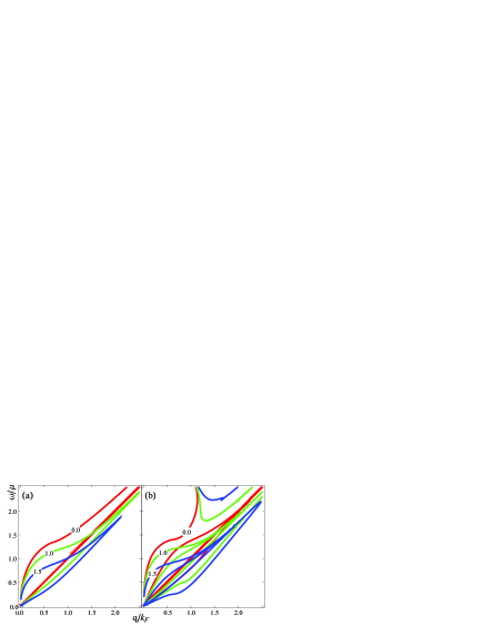
Figure 1: (Color online) Undamped (two higher frequency branches) and damped (two lower in frequency branches) plasmon dispersion relations for gapped graphene. The curves in (a) correspond to 0ML(single layer), the curves in (b) to 1ML(double layer) configuration. The red, green and blue curves show the plasmon dispersion for $E_{g}/\mu=\left\{{0.0,1.0,1.5}\right\}$, respectively.

The plasmon branches for $k_{F}d=1$ and several values of $E_{g}$ are presented in Fig. 1. In the long-wavelength limit the single graphene layer (0ML) exhibits a single undamped plasmon branch [Fig. 1(a)] given by

$$\omega_{p}^{2}=q\mathcal{D}(E_{g})\ ,$$ (33)

where the plasmon Drude factor is defined as

$$\mathcal{D}(E_{g})=\frac{2\mu e^{2}}{\hbar^{2}\epsilon_{\texttt{SiC}}}\left[{1-(E_{g}/2\mu)^{2}}\right]\ .$$ (34)

In the double layer configuration (1ML), there are two plasmon branches, i.e., the symmetric $\omega_{+}$ and asymmetric $\omega_{-}$ modes. For large interlayer distance $k_{F}d\gg 1$, the two branches are qualitatively similar and given by

$$\omega^{2}_{+}=q\mathcal{D}(0)\ ,$$ (35)

$$\omega^{2}_{-}=q\mathcal{D}(E_{g})\ .$$

In the opposite limit of closely placed layers with $k_{F}d\ll 1$, the asymmetric branch becomes acoustic with frequency defined by

$$\omega^{2}_{-}=2dq^{2}\mathcal{D}(E_{g})\ .$$ (36)

We note that the asymmetric branch is always smaller in frequency than symmetric mode. In the next section, we shall combine Eqs. (28), (29) with (32) and simulate the energy loss for two distinct cases, namely when the charged particle motion is parallel and perpendicular to the graphene layers.

IV Numerical results and Discussion

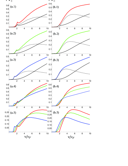
Figure 2: (Color online) Stopping power, as a function of charged particle velocity in units of $(Ze/2\pi)^{2}\epsilon_{s}^{-1}$. Rows (a), (b) correspond to double and single layer configurations, respectively. Panels (1), (2) and (3) correspond to $E_{g}/\mu=\left\{{0.0,1.0,1.5}\right\}$ illustrated by red, green and blue curves, respectively. The solid black curve is the particle-hole contribution, and the dashed curve shows the plasmon contribution. Row (4) gives the particle-hole contribution for the three values of the gap, and row (5) shows the associated plasmon contributions.

We begin our discussion with the energy loss rates in Eq. (13) for single and symmetric double layer configurations. Our energy loss results for charged particle motion parallel to the surface are shown in Fig. 2. The separation between the two layers was chosen as $k_{F}d=1.0$. The charged particle travels above the graphene surface at a height $k_{F}z_{1}=2.0$. All frequencies were analytically continued to the complex plane and acquire a small positive loss rate $\omega\rightarrow\omega+i\gamma$ with $\gamma/\mu=10^{-4}$. We notice that the plasmon contribution becomes smaller with increasing energy gap $E_{g}$. This can be easily attributed to decreasing plasmon Drude factor $\mathcal{D}(E_{g})$. The contribution from the particle-hole modes is largely unaffected by the gap. In the double layer configuration, a small spike at the beginning of the plasmon contribution region is due to the two branches. Both undamped optical and acoustic plasmon branches contribute. However, with increased particle velocity, only the optical branch contributes, as it is demonstrated in Fig. 1. Since the spectral weight of the optical branch is larger than that of the acoustic branch, we see that the spike appears. We note that one can obtain a closed-form analytic expression for the loss rate if we include only the long wavelength plasmon contributions. fessatidis In any event, this must be the leading contribution for small and moderate particle velocities $v_{\parallel}/v_{F}<6$, because of the $\texttt{e}^{-qz_{1}}/q$ factor.

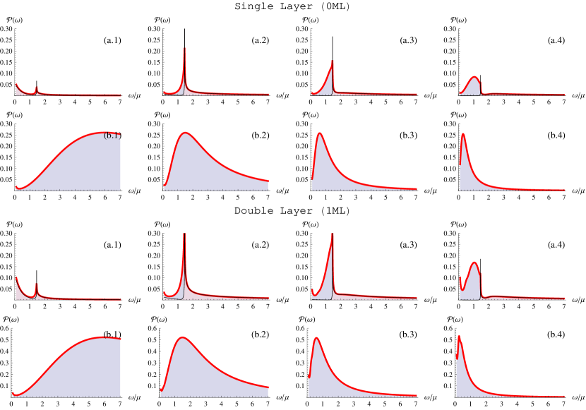
Figure 3: (Color on-line) Energy loss spectra of the charged particle transmitted through single and double $(k_{F}d=100)$ free-standing graphene. Rows (a) and (b) correspond to the full version of the RPA polarization and its long-wave plasmon approximation, respectively. In columns (1) through (4), the charged particle speed increases as $v_{z}/v_{F}=\left\{{0.5,2.0,5.0,10.0}\right\}$. The thin black curves correspond to particle-hole (and damped plasmon) contributions only.

We now consider a single, free-standing $(E_{g}=0)$ and double-layer graphene and present results for the energy loss spectra of a charged particle moving perpendicular to the graphene surface. By symmetry, the transmission and reflection spectra from the single layer must be identical. The transmission spectra are shown in Fig. 3. The energy loss was calculated using either the full version of the noninteracting polarization function in the RPA (32) shown in Fig. 3(a), or its long-wavelength plasmon pole approximation [Eqs. (33) and (35)] as seen in Fig. 3(b). One may classify three different scattering regimes depending on the charged particle velocity $v_{z}/v_{F}$. In the low-velocity regime, as shown in column (1) of Fig. 3 for single and double layers, the particle-hole excitations dominate the scattering. There is an absorption spike due to the Landau damped plasmon mode which separates the particle-hole continuum from the undamped plasmon modes as shown in Fig. 1(a). The strength of the spike diminishes with increased charged particle speed. The position of such resonance absorption at $(\approx 1.5)$ is independent of $v_{z}$, indicating the effect due to linear dispersion of the damped plasmon branch. In the intermediate velocity regime given in columns (2) and (3) of Fig. 3, the damped and undamped plasmon mode contributions are comparable. However, in the high-velocity limit, shown in columns (4) of Fig. 3, the undamped plasmons dominate the spectra. In that regime, one can employ the polarization in its long wave limit to a good approximation, as we can see in Fig. 3(b). The approximation works for both the single and double-layer configuration. In the work of Allison, et al., Miskovic an attempt was made to compensate for the red shift of the absorption maximum by introducing a restoring force in the electron liquid. However, the origin of this restoring force was not clear. Additionally, the approximation introduced in their work does not yield results which converge on those when the RPA polarization for graphene is employed. Another observation is that the double layer just doubles the absorption of the single layer, without any perceptible spectral shift. This is a consequence of large interlayer distance. When the layers are closely packed the absorption peak is blue shifted with increasing number of layers, in agreement with Ref. LU:2009,

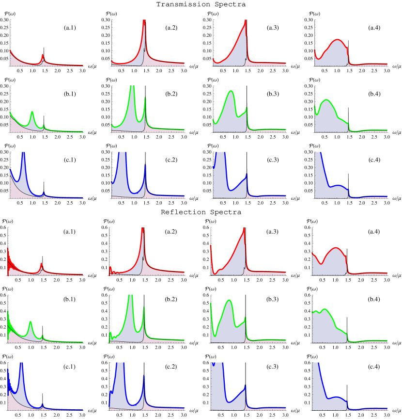
Figure 4: (Color on-line) Energy loss spectra of the charged particle transmitted through and reflected from a double $(k_{F}d=100)$ epitaxial graphene. Rows (a) through (c) are for increasing energy gap on the zeroth layer with $E_{g}/\mu=\left\{{0.5,1.0,1.5}\right\}$. In columns (1) through (4), the charged particle speed increases as $v_{z}/v_{F}=\left\{{0.5,2.0,5.0,10.0}\right\}$. The thin black curves correspond to particle-hole (and damped plasmon) contributions only. The color schematic correspond to Fig. 1 and Fig. 2.

In Fig. 4, we present the transmission and reflection spectra for epitaxial MLG. The zeroth layer only acquires the energy gap. This gap increases in columns (1) through (3). Our principal observation is that in the intermediate velocity regime, given by columns (2) and (3) in Fig. 4, the absorption spectrum splits into two peaks. The one identified with the damped plasmon peak ($\hbar\omega/\mu\approx 1.5$) comes from the upper graphene layer for which $E_{g}=0$. The other peak may be attributed to the symmetry-broken zeroth layer absorption ($E_{g}\neq 0$). We note that in the high velocity limit, shown in column (4) of Fig. 4, the gap results in a red shift of the absorption maximum. The small splitting of the peak is also visible on the damped plasmon contribution. As a matter of fact, the layers are so far apart that one cannot identify a plasmon mode as the acoustic branch. The reflection spectrum qualitatively mimics the transmitted spectrum, but doubles in height. This is because the charged particle spends twice as much time in between the layers compared to the transmissive case. Of course, the particle expends most of its energy on this part of the trajectory.

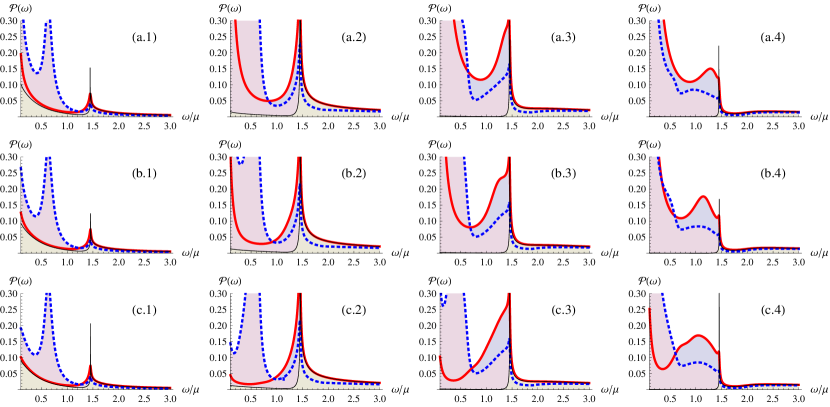
Figure 5: (Color online) Energy loss spectra of the charged particle transmitted through a double free-standing graphene. Rows (a) through (c) correspond to increasing interlayer distance $k_{F}d=\left\{{5,10,50}\right\}$ . In columns (1) through (4), the charged particle speed increases as with $v_{z}/v_{F}=\left\{{0.5,2.0,5.0,10.0}\right\}$. The thin black curves correspond to particle-hole (and damped plasmon) contributions only. Red thick and Blue dotted curves stand for $E_{g}/\mu=0.0$ and $E_{g}/\mu=1.5$ correspondingly.

To see the acoustic branch (Fig. 1(b)) in the spectra, we vary intralayer distance in (rows (a) through (c) of Fig. 5. for all velocity regimes [panels (1)-(4)]. Several values of the gap are also shown on the graph. The low-frequency acoustic branch boosts the long wavelength absorption ($\hbar\omega/\mu\approx 0$). This is especially so for small energy gap, since the separation between the branches is well pronounced [Fig. 1(b)]. In the high velocity regime or result os small interlayer separation [Fig. 5 (a.4)] ore result is qualitatively similar to Fig.3 of Ref. LU:2009, . With increasing angle of incidence $\theta_{i}=\texttt{tan}^{-1}(v_{\parallel}/v_{z})$ the sharp peak of the particle hole absorption becomes less pronounced and finally reaches the smooth curve as in Fig. 2(a.1- a.4). The plasmon peak is blue shifted with $\texttt{sin}\theta_{i}$ finally reaching those of Fig. 2(a.5). Since the plasmon momentum is proportional to $\texttt{sin}\theta_{i}$ one can interpret this blue shift as the Raman shift due to plasmon activation. Given its linear nature we deuce that for small interlayer distance mostly acoustic plasmon branch is activated, thus explaining Fig.2(d) of Ref. LU:2009, . This interpretation is further confirmed by the comparison with the large interlayer separation Raman shift, which follows $\sqrt{\texttt{sin}\theta_{i}}$ pattern. Unfortunately, as it follows from Fig. 1(b), it is hard to deduce existence of the gap from the acoustic plasmon branch. Experimentally one would have to transfer MLG onto a non-polar substrate and observe the increase in the plasmon slope if the gap was originally present.

Comparing the plasmon absorption in the parallel and perpendicular cases, the plasmons contribute more to the former in the low-velocity regime, whereas in the latter case, their contribution is most pronounced for higher incoming charged particle velocities.

V Summary

We have investigated the role played by a gap in the energy dispersion on the absorption spectra of single and double layer configurations. All velocity regimes for the external charged particle moving perpendicular to the graphene surface were reported in Figs. 3, 4 and 5. The plasmon pole approximation for the polarization agrees well with the results obtained with the full polarization in the RPA in the high-velocity regime only. The speed of the external charged particle determines whether the plasmon or particle-hole excitations dominate the scattering. Consequently, since gapped graphene has a different plasma excitation spectrum than free-standing graphene, its stopping power may carry distinct signatures of the substrate induced gap. We also demonstrated that our formalism can qualitatively describe experimental data of ELLS. It also allowed us to interpret the observed linear plasmon dispersion as coming from the acoustical undamped branch.

Appendix A An alternative derivation of the energy loss formula

Here, we derive Eq.(17) by a method similar to that in Refs. Mills, and Miskovic, . First, we introduce the 2D Fourier transform and its inverse given by

$$\left[{\mathcal{F}_{2D,\alpha}f}\right](\mathbf{q}_{\alpha\parallel},z_{\alpha},\omega_{\alpha})=\int\limits_{-\infty}^{\infty}dt_{\alpha}\ \texttt{e}^{i\omega_{\alpha}t_{\alpha}}\int d^{2}\mathbf{r}_{\alpha\parallel}\ \texttt{e}^{-i\mathbf{q}_{\alpha,\parallel}\cdot\mathbf{r}_{\alpha\parallel}}f\left({\mathbf{r}_{\alpha\parallel},z_{\alpha},t_{\alpha}}\right)\ ,$$ (37)

$$\left[{\mathcal{F}^{-1}_{2D,\alpha}f}\right](\mathbf{r}_{\alpha\parallel},z_{\alpha},t_{\alpha})=\frac{1}{\left({2\pi}\right)^{3}}\int\limits_{-\infty}^{\infty}d\omega_{\alpha}\texttt{e}^{-i\omega_{\alpha}t_{\alpha}}\int d^{2}\mathbf{q}_{\alpha\parallel}\texttt{e}^{i\mathbf{q}_{\alpha\parallel}\cdot\mathbf{r}_{\alpha\parallel}}f\left({\mathbf{q}_{\alpha\parallel},z_{\alpha},\omega_{\alpha}}\right)\ ,$$ (38)

where we have adopted the notation of Camley and Mills Mills with $\alpha=1,2$. By applying such a Fourier transformation defined in (38) to the Poisson equation (3), we obtain after some straightforward algebra the following differential equation

$$\left({\frac{\partial^{2}}{\partial z^{2}_{2}}-q^{2}_{2\parallel}}\right)\Phi_{\texttt{ext}}\left({\mathbf{q}_{2\parallel},z_{2},\omega_{2}}\right)=-\frac{Ze}{v_{z}\epsilon_{0}}\,\texttt{e}^{i\left({\omega_{2}-\mathbf{q}_{2\parallel}\cdot\mathbf{v}_{\parallel}}\right)z_{2}/v_{z}}\ .$$ (39)

By applying the boundary conditions $\Phi_{\texttt{ext}}\left({\mathbf{q}_{2\parallel},\pm\infty,\omega_{2}}\right)=0$, the solution may be written as

$$\Phi_{\texttt{ext}}\left({\mathbf{q}_{2\parallel},z_{2},\omega_{2}}\right)=\frac{Ze\,v_{z}\,\texttt{e}^{i\left({\omega_{2}-\mathbf{q}_{2\parallel}\cdot\mathbf{v}_{\parallel}}\right)z_{2}/v_{z}}}{\epsilon_{0}\left[\left({q_{2\parallel}v_{z}}\right)^{2}+\left({\omega_{2}-\mathbf{q}_{2\parallel}\cdot\mathbf{v}_{\parallel}}\right)^{2}\right]}\ .$$ (40)

Therefore, the external potential assumes the form

$$\Phi_{\texttt{ext}}\left({\mathbf{r}_{2\parallel},z_{2},t_{2}}\right)=\mathcal{F}^{-1}_{2d,2}\Phi_{\texttt{ext}}\left({\mathbf{q}_{2\parallel},z_{2},\omega_{2}}\right)$$ (41)

$$=\frac{Ze\,v_{z}}{\left({2\pi}\right)^{3}\epsilon_{0}}\int\limits_{-\infty}^{\infty}d\omega_{2}\,\texttt{e}^{-i\omega_{2}t_{2}}\int d^{2}\mathbf{q}_{2\parallel}\ \frac{\exp\left({i\mathbf{q}_{2\parallel}\cdot\mathbf{r}_{2\parallel}+i\left({\omega_{2}-\mathbf{q}_{2\parallel}\cdot\mathbf{v}_{\parallel}}\right)z_{2}/v_{z}}\right)}{\left({q_{2\parallel}v_{z}}\right)^{2}+\left({\omega_{2}-\mathbf{q}_{2\parallel}\cdot\mathbf{v}_{\parallel}}\right)^{2}}\ .$$

Similarly, we make a Fourier representation for the nonlocal inverse dielectric function as

$$\epsilon^{-1}\left({\mathbf{r}_{1\parallel},z_{1},t_{1};\mathbf{r}_{2\parallel},z_{2},t_{2}}\right)=\epsilon^{-1}\left({z_{1},z_{2};\mathbf{r}_{1\parallel}-\mathbf{r}_{2\parallel},t_{1}-t_{2}}\right)$$ (42)

$$=\frac{1}{\left({2\pi}\right)^{3}}\int\limits_{-\infty}^{\infty}d\omega\ \texttt{e}^{-i\omega(t_{1}-t_{2})}\int d^{2}\mathbf{q}_{\parallel}\ \texttt{e}^{i\mathbf{q}_{\parallel}\cdot(\mathbf{r}_{1\parallel}-\mathbf{r}_{2\parallel})}\,\epsilon^{-1}\left({z_{1},z_{2};\mathbf{q}_{\parallel},\omega}\right)\ .$$

Combining Eqs. (41) and (42) with Eq. (2), we obtain

$$\Phi_{\texttt{tot}}\left({\mathbf{r}_{1\parallel},z_{1},t_{1}}\right)=\frac{Ze\,v_{z}}{\left({2\pi}\right)^{3}\epsilon_{0}}\int\limits_{-\infty}^{\infty}d\omega\ \texttt{e}^{-i\omega t_{1}}\int d^{2}\mathbf{q}_{\parallel}\ \texttt{e}^{i\mathbf{q}_{\parallel}\cdot\mathbf{r}_{1\parallel}}\int\limits_{-\infty}^{\infty}dz_{2}$$ (43)

$$\times\epsilon^{-1}\left({z_{1},z_{2};\mathbf{q}_{\parallel},\omega}\right)\frac{\exp\left({i\left({\omega-\mathbf{q}_{\parallel}\cdot\mathbf{v}_{\parallel}}\right)z_{2}/v_{z}}\right)}{\left({q_{\parallel}v_{z}}\right)^{2}+\left({\omega-\mathbf{q}_{\parallel}}\cdot\mathbf{v}_{\parallel}\right)^{2}}\ .$$

Here, we used the following identities:

$$\int\limits_{-\infty}^{\infty}dt_{2}\ \texttt{e}^{-i(\omega_{2}-\omega)t_{2}}=2\pi\delta\left({\omega_{2}-\omega}\right)\ ,$$

$$\int d^{2}\mathbf{r}_{2\parallel}\,\texttt{e}^{-i(\mathbf{q}_{\parallel}-\mathbf{q}_{2\parallel})\cdot\mathbf{r}_{2\parallel}}\left({2\pi}\right)^{2}\delta\left({\mathbf{q}_{\parallel}-\mathbf{q}_{2\parallel}}\right)\ .$$

The force acting on the particle is given by combining Eq. (43) and Eq. (1), with the replacement $\nabla_{1}=\partial/\partial\mathbf{v}t_{1}$. The resulting expression is inserted into Eq. (6), yielding

$$W_{\theta}\left({\mathbf{v}}\right)=\int\limits_{-\infty}^{\infty}d(\mathbf{v}\,z_{1}/v_{z})\cdot\mathbf{F}\left({1}\right)=-\frac{(Ze)^{2}}{\left({2\pi}\right)^{3}\epsilon_{0}}\int\limits_{-\infty}^{\infty}dz_{1}\int\limits_{-\infty}^{\infty}dz_{2}\int d^{2}\mathbf{q}_{\parallel}\int\limits_{-\infty}^{\infty}d\omega\ i\omega\,\texttt{e}^{-i\omega z_{1}/v_{z}}\,\texttt{e}^{i\mathbf{q}_{\parallel}\cdot\mathbf{v}_{\parallel}z_{1}/v_{z}}$$ (44)

$$\times\epsilon^{-1}\left({z_{1},z_{2};\mathbf{q}_{\parallel},\omega}\right)\frac{\exp\left({i\left({\omega-\mathbf{q}_{\parallel}\cdot\mathbf{v}_{\parallel}}\right)z_{2}/v_{z}}\right)}{\left({q_{\parallel}v_{z}}\right)^{2}+\left({\omega-\mathbf{q}_{\parallel}}\cdot\mathbf{v}_{\parallel}\right)^{2}}$$

$$=-\frac{(Ze)^{2}}{\left({2\pi}\right)^{3}\epsilon_{0}}\int\limits_{-\infty}^{\infty}dz_{1}\int\limits_{-\infty}^{\infty}dz_{2}\int d^{2}\mathbf{q}_{\parallel}\int\limits_{-\infty}^{\infty}d\omega\ i\omega\,\epsilon^{-1}\left({z_{1},z_{2};\mathbf{q}_{\parallel},\omega}\right)\frac{\exp\left[{i\left({\omega-\mathbf{q}_{\parallel}\cdot\mathbf{v}_{\parallel}}\right)(z_{2}-z_{1})/v_{z}}\right]}{\left({q_{\parallel}v_{z}}\right)^{2}+\left({\omega-\mathbf{q}_{\parallel}}\cdot\mathbf{v}_{\parallel}\right)^{2}}\ .$$

Now, let us change the dummy variables $\omega\to-\omega\;\mathbf{q}_{\parallel}\rightarrow-\mathbf{q}_{\parallel}$ in the above equation and utilize the symmetry relation in Eq. (11). We obtain

$$W_{\theta}\left({\mathbf{v}}\right)=\frac{2(Ze)^{2}}{\left({2\pi}\right)^{3}\epsilon_{0}}\ \Im\texttt{m}\int\limits_{-\infty}^{\infty}dz_{1}\int\limits_{-\infty}^{\infty}dz_{2}\int d^{2}\mathbf{q}_{\parallel}\int\limits_{0}^{\infty}d\omega\ \omega\,\epsilon^{-1}\left({z_{1},z_{2};\mathbf{q}_{\parallel},\omega}\right)\frac{\exp\left[{i\left({\omega-\mathbf{q}_{\parallel}\cdot\mathbf{v}_{\parallel}}\right)(z_{2}-z_{1})/v_{z}}\right]}{\left({q_{\parallel}v_{z}}\right)^{2}+\left({\omega-\mathbf{q}_{\parallel}}\cdot\mathbf{v}_{\parallel}\right)^{2}}\ .$$ (45)

References

• (1) R. H. Ritchie, Phys. Rev. 106, 874 (1957).
• (2) G. Gumbs and N. J. M. Horing, Phys. Rev. B43, 2119 (1991).
• (3) Vassilios Fessatidis, Norman J.M. Horing, Antonios Balassis, Phys. Lett. A 375, 192 (2010).
• (4) N. J. M. Horing, H. C. Tso, and G. Gumbs, Phys. Rev. B 36, 1588 (1987).
• (5) G. Gumbs and A. Balassis, Phys. Rev. B 71, 235410 (2005).
• (6) B. Wunsch, T. Stauber, F. Sols, and F. Guinea, New Journal of Physics. 8, 318 (2006).
• (7) O. V. Kibis, Phys. Rev. B, 81, 165433 (2010)).
• (8) O. Roslyak, G. Gumbs, and D. H. Huang, J. Appl. Phys. (submitted).
• (9) Xue-Feng Wang and Tapash Chakraborty, Phys. Rev. B75, 033408 (2007).
• (10) P. K. Pyatkovskiy, J. Phys.: Condens. Matter 21, 025506 (2009).
• (11) G. Li, A. Luican, and E.Y. Andrei, Phys. Rev. Lett. 102, 176804 (2009).
• (12) G. Giovannetti, et. al., Phys. Rev. B., 76, 073103, (2007).
• (13) K. W-K. Shung, Phys. Rev. B 34, 979 (1986).
• (14) K. W-K. Shung, Phys. Rev. B 34, 1264 (1986).
• (15) M. Sprinkle et.al., ArXiv:1001.3869v1 (20010), Phys. Rev. Lett., 103, 226803 (2009).
• (16) A. Mattausch and O. Pankratov, Phys. Rev. Lett., 99 076802 (2007).
• (17) P. Mallet et.al., Phys. Rev. B., 76 041403(R) (2007).
• (18) E. Rotenberg, et. al., Nature Matter. 7, 258 (2008).
• (19) S. Kim, J. Ihm, H. J. Choi, and Y. Son, Phys. Rev. Lett. 100, 176802 (2008).
• (20) S. Y. Zhou et al., Nature Matter. 6, 770 (2007).
• (21) A. Bostwick et al., Nature Phys. 3, 36 (2007).
• (22) J. Lu and K. P. Loh, Phys. Rev. B., 80 113410 (2009).
• (23) M. S. Kushwaha, Surface Science Reports 41, 1 (2001).
• (24) , G. Gumbs, Sol,. State Commun. 65, 393 (1988).
• (25) R. E. Camley and D. L. Mills, Phys. Rev. B 26, 1280 (1982).
• (26) K. F. Allison, D. Borka, I. Radovic, L. Hadzievski, and Z. L. Miskovic, Phys. Rev. B 80, 195405 (2009).
• (27) Y. Liu and R. F. Wills, Phys. Rev. B., 81 081406 (2010).
• (28) C. Tegenkamp et.al., J. Phys.: Condens. Matter, 23 012001 (2011).
Refer to caption