Hopf bifurcations to quasi-periodic solutions
for the two-dimensional plane Poiseuille flow

Abstract

This paper studies various Hopf bifurcations in the two-dimensional plane Poiseuille problem. For several values of the wavenumber $\alpha$, we obtain the branch of periodic flows which are born at the Hopf bifurcation of the laminar flow. It is known that, taking $\alpha\approx 1$, the branch of periodic solutions has several Hopf bifurcations to quasi-periodic orbits. For the first bifurcation, previous calculations seem to indicate that the bifurcating quasi-periodic flows are stable and go backwards with respect to the Reynolds number, $Re$. By improving the precision of previous works we find that the bifurcating flows are unstable and go forward with respect to $Re$. We have also analysed the second Hopf bifurcation of periodic orbits for several $\alpha$, to find again quasi-periodic solutions with increasing $Re$. In this case the bifurcated solutions are stable to superharmonic disturbances for $Re$ up to another new Hopf bifurcation to a family of stable $3$-tori. The proposed numerical scheme is based on a full numerical integration of the Navier-Stokes equations, together with a division by 3 of their total dimension, and the use of a pseudo-Newton method on suitable Poincaré sections. The most intensive part of the computations has been performed in parallel. We believe that this methodology can also be applied to similar problems.

I Introduction

The theory of hydrodynamic stability is one of the main topics in fluid mechanics. Poiseuille as well as Taylor–Couette flow are test problems where it is possible the evaluation of different analytical and numerical methods, due essentially to the simplicity of their geometry. The dynamics of plane Poiseuille flow departs from the laminar flow. The stability of the laminar solution to infinitesimal disturbances has been analysed linearly and gives rise to the Orr–Sommerfeld equation. This equation has been studied by several authors as Thomas (1953), Orszag (1971), and Maslowe (1985) among others, and it is well understood. The critical Reynolds number of the linear theory, $Re_{cr}=5772.22$ for the wavenumber $\alpha=1.02056$, has been obtained by this approach. However, as experiments of Carlson, Widnall, and Peeters Carlson et al. (1982), Nishioka and Asai (1985), and Alavyoon, Henningson, and Alfredsson Alavyoon et al. (1986) showed, transition to turbulence is observed for Reynolds number $\approx 1000$, what motivates that finite-amplitude disturbances originate the transition. The understanding of the transition to turbulence has been conjectured by Saffman (1983) to depend on intermediate vortical states and turbulence takes place due to their three-dimensional instability. In recent years, authors have also payed attention to subcritical transition models based on transient optimal growth (see Schmid and Henningson (2001), for instance). Examples of vortical states are periodic flows in time or space, among which can be mentioned: two-dimensional travelling waves, secondary flows in two or three dimensions (for them the flow rate and the pressure gradient are constants) and quasi-periodic solutions. Ehrenstein and Koch (1991) discovered a new family of secondary bifurcation branches in dimension 3, which contains only even spanwise Fourier modes and reduces the critical Reynolds number (defined in terms of the averaged velocity across the channel) to $Re_{Q_{m}}\approx 1000$ as observed in experiments.

Two-dimensional disordered motion is associated with the large scales of some turbulent flows, so there probably exist attractors for those two-dimensional flows. Besides, two- and three-dimensional states can compete and coexist in the final flow (cf. Jiménez (1987) and the references therein). In spite of the fact that transition to turbulence is a three-dimensional phenomenon, there are many properties of the two-dimensional flows observed in fully turbulent three-dimensional flows such as wall sweeps, ejections, intermittency and bursting, as Jiménez (1990) showed. The two-dimensional case has attracted the attention of many authors but it is not completely understood as the problem of two-dimensional transition to turbulence proves. Due to Squire’s Squire (1933) theorem, to every three-dimensional perturbation of the linearized Navier–Stokes equations for a given $Re,\alpha$, it corresponds a two-dimensional one for some $\tilde{\alpha}\geqslant\alpha$ and $\tilde{Re}\leqslant Re$, so the critical $Re$ for the linear theory must be attained by a two-dimensional flow. This result has been one of the main reasons to firstly try to understand the two-dimensional case, apart from the obvious easiness of computations compared to the three-dimensional situation. In addition, some of the properties obtained from the two-dimensional case can also provide new insight for three-dimensional flows.

In this work we intend to analyse the dynamics of an easily treatable problem without domain complexities as is the case of the two-dimensional plane Poiseuille flow. Different levels of bifurcation to respective vortical states are considered, starting at the basic parabolic flow. From it, a family of travelling waves is born subcritically (see  ​§ IV.3) for $\alpha\approx 1$. There are many papers concerning this kind of waves: Soibelman and Meiron (1991) gave an excellent review about it. As a starting point for our computations we have also reproduced the calculations to find the travelling waves for several values of $\alpha$. Jiménez (1987, 1990) and Soibelman and Meiron (1991) obtained the next level of bifurcation to quasi-periodic solutions. Employing full numerical simulation in time, Jiménez (1987, 1990) computed different attractor flows with a moderate number of Chebyshev and Fourier modes. On the other hand, Soibelman and Meiron (1991) implemented an algebraic approach to capture stable and unstable quasi-periodic flows, but the number of modes used were not enough to give good results and they were not able to carry out the stability analysis. The method implemented in the present work combines both: we solve a stationary problem to compute travelling waves for an observer moving at an appropriate speed, whereas the quasi-periodic flows are found by means of full numerical integration of the Navier–Stokes equations. Through algebraic manipulations, we express the discretized Navier–Stokes system only in terms of the stream component of the velocity. As a consequence, the dimension of the system is divided by 3, reducing considerably the computational effort. Using the numerical integrator, we have built a Poincaré section of the flow, in order to apply a pseudo-Newton method for obtaining also unstable quasi-periodic solutions. These unstable intermediate states of the flow provide a highly useful insight into the transition process, as exemplified by secondary bifurcations in shear flows (see Casas and Jorba (2004) for instance). The spatio-temporal symmetries of the channel allows the reduction of quasi-periodic flows with two-frequencies to periodic flows in the appropriate Galilean reference. The quasi-periodic solutions found in this work correspond to the first two Hopf bifurcations of travelling waves for the case of constant pressure drop through the channel, and the first Hopf bifurcation when the mass flux is held constant. The property of behaving as time-periodic flows if we take a suitable Galilean reference, simplifies enormously the search of this kind of solutions. For them, the associated return time to the Poincaré section is roughly $10000$ time units at the first Hopf bifurcation for constant pressure, what makes the temporal integration very costly. The considered numerical procedure utilizes a parallel algorithm to evaluate the different columns of a Jacobian matrix, needed in the application of pseudo-Newton’s method for the continuation of quasi-periodic solutions. We find that on the analysed Hopf bifurcations for both constant pressure and constant flux formulations, there exist quasi-periodic flows with increasing $Re$ for some range of $\alpha$ and with decreasing $Re$ for some other $\alpha$: the bifurcations are supercritical or subcritical respectively. On the first bifurcation for constant pressure, we have traversed a curve of unstable quasi-periodic solutions. On the remaining bifurcations, there are stable quasi-periodic solutions to disturbances with the same wavenumber $\alpha$ and likewise, for $Re$ sufficiently large, we have obtained unstable solutions.

Once we have situated the different studies concerning Poiseuille flow, in the next section we pose the concrete terms that define the plane Poiseuille problem in two dimensions, together with their equations for both cases of constant pressure and flux. Next in ​§ III we explain the main details of the numerical methods. In ​§ IV we review some results of the Orr–Sommerfeld equation and obtain, for several values of $\alpha$, the bifurcating solutions of time-periodic flows. From these we analyse in ​§ V the bifurcating branches to quasi-periodic solutions at the above-mentioned Hopf bifurcations. Finally in ​§ VI we point out some conclusions.

II Poiseuille flow

We consider the flow of a viscous incompressible two-dimensional fluid, in a channel between two parallel walls, governed by the Navier–Stokes equations together with the incompressibility condition

$$\frac{\partial{\bf u}}{\partial t}+({\bf u}\boldsymbol{\cdot}\boldsymbol{\nabla}){\bf u}=-\nabla p+\frac{1}{Re}\Delta{\bf u},\qquad\boldsymbol{\nabla}\boldsymbol{\cdot}{\bf u}=0,$$ (1)

where ${\bf u}={\bf u}(x,y,t)=(u,v)(x,y,t)$ represents the two-dimensional velocity, $p=p(x,y,t)$ the pressure and $Re$ the Reynolds number. As boundary conditions we suppose no-slip on the channel walls at $y=\pm 1$ and, at artificial boundaries in the stream direction $x$, a period $L$, i.e.

$$\left.\begin{matrix}\hfill u(x,\pm 1,t)=v(x,\pm 1,t)=0\cr\hfill(u,v,p^{\prime})(x+L,y,t)=(u,v,p^{\prime})(x,y,t)\cr\end{matrix}\right\}\qquad x\in\mathbb{R},\quad y\in[-1,1],\quad t\geqslant 0,$$ (2)

being $p^{\prime}=p+Gx$, for $G=G(t)$ the mean pressure gradient on the channel length, $L$, in the streamwise direction. For the system previously described there is a time-independent solution known as the basic or laminar flow that has a parabolic profile, namely

$$u_{b}(y)=1-y^{2},\quad v_{b}=0,\quad\nabla p_{b}=(-\frac{2}{Re},0).$$

Magnitudes in (1)–(2) are non-dimensional. We consider the two typical formulations used to drive the fluid: fixing the total flux $Q$, or the mean pressure gradient $G$, through the channel. For each of them we obtain a different definition of $Re=hU_{c}/\nu$ namely, $Re_{Q}=3Q/4\nu$ and $Re_{p}=Gh^{3}/2\rho\nu^{2}$ respectively, where, in dimensional magnitudes, $h$ represents half of the channel height, $U_{c}$ the velocity of the laminar flow in the centre of the channel, and $\nu$ and $\rho$ the constant kinematic viscosity and density. For a given laminar flow, i.e. letting $U_{c}$ fixed, both definitions of the Reynolds number coincides with $Re=hU_{c}/\nu$. That is not the case for secondary flows, defined as the ones having constant flux and mean pressure gradient through the channel. If we consider such a flow ${\bf u}(x,y)$, expressed for each formulation by means of respective Fourier series

$${\bf u}^{Q}(x,y)=\sum_{k\in\mathbb{Z}}\hat{{\bf u}}_{k}^{Q}(y)\mathrm{e}^{\mathrm{i}k\alpha x},\qquad{\bf u}^{p}(x,y)=\sum_{k\in\mathbb{Z}}\hat{{\bf u}}_{k}^{p}(y)\mathrm{e}^{\mathrm{i}k\alpha x},$$

then, using the notation $[f]_{a}^{b}:=f(b)-f(a)$, it is easy to check that (see for instance Casas (2002))

$$\frac{Re_{p}}{Re_{Q}}=-\frac{1}{4}\left[\frac{\partial{\hat{u}}_{0}^{Q}}{\partial y}\right]_{-1}^{1},\qquad\frac{Re_{Q}}{Re_{p}}=\frac{3}{4}\int_{-1}^{1}u^{p}(x,y)\,\mathrm{d}y,$$ (3)

and the corresponding relationships between velocities and pressures

$${\bf u}^{p}(x,y)=\frac{Re_{Q}}{Re_{p}}{\bf u}^{Q}(x,y),\qquad p^{p}(x,y)=\frac{Re_{Q}^{2}}{Re_{p}^{2}}p^{Q}(x,y).$$ (4)

We will employ later that periodic conditions at artificial boundaries in the stream direction, yield a great simplification in the structure of the flow: quasi-periodic solutions may be viewed as periodic flows, and periodic solutions as stationary ones, if the observer moves at adequate speed $c$, in the stream direction. For this reason we perform the change of variable $\tilde{x}=x-ct$, which (writing again $x$ instead of $\tilde{x}$) turns system (1) into:

$$\left\{\begin{array}[]{r@{\hspace{0,5ex}}l}\displaystyle\frac{\partial u}{\partial t}+(u-c)\frac{\partial u}{\partial x}+v\frac{\partial u}{\partial y}\hskip 2.15277pt&=\displaystyle-\frac{\partial p}{\partial x}+\frac{1}{Re}\left(\frac{\partial^{2}u}{\partial x^{2}}+\frac{\partial^{2}u}{\partial y^{2}}\right)\\[12.91663pt] \displaystyle\frac{\partial v}{\partial t}+(u-c)\frac{\partial v}{\partial x}+v\frac{\partial v}{\partial y}\hskip 2.15277pt&=\displaystyle-\frac{\partial p}{\partial y}+\frac{1}{Re}\left(\frac{\partial^{2}v}{\partial x^{2}}+\frac{\partial^{2}v}{\partial y^{2}}\right)\\[12.91663pt] \displaystyle\frac{\partial u}{\partial x}+\frac{\partial v}{\partial y}\hskip 2.15277pt&=0,\end{array}\right.$$ (5)

together with boundary conditions as in (2). We can recover (1) by simply taking $c=0$ in (5).

III Numerical approach

Let us now describe the numerical procedure. For system (5) we want to follow the temporal evolution of an initial flow subjected to the incompressibility condition, $\boldsymbol{\nabla}\boldsymbol{\cdot}{\bf u}=0$, and boundary conditions (2). To this end we use a spectral method to approximate velocities $u,v$ and pressure deviation $p^{\prime}$, which from now on we consider non-dimensional quantities. We recall that $p=p^{\prime}-Gx$ and as it is easily obtained (see for example Casas (2002))

$$G=-\frac{1}{2Re_{Q}}\left[\frac{\partial\hat{u}_{0}}{\partial y}\right]_{-1}^{1}\quad\mbox{or}\quad G=\frac{2}{Re_{p}},$$ (6)

respectively for the constant flux or pressure cases, so in the first one the mean pressure gradient varies with time and it is constant for the second one.

Spatial discretization. We use a standard Fourier-Galerkin, Chebyshev-collocation approach (cf. Canuto et al. (1988)) in order to discretize $x,y$ derivatives. In this way, we consider Fourier series (with $\alpha=2\pi/L$ the parameter wavenumber):

$$(u,v,p^{\prime})(x,y,t)=\sum_{k=-N}^{N}(\hat{u}_{k},\hat{v}_{k},\hat{p}_{k})(y,t)\mathrm{e}^{\mathrm{i}k\alpha x},\qquad x\in\mathbb{R},\quad y\in[-1,1],\quad t\geqslant 0,$$

which substituted in (5) gives rise to a system of partial differential equations for the Fourier coefficients $(\hat{u}_{k},\hat{v}_{k},\hat{p}_{k})$,

$$\left\{\begin{array}[]{r@{\hspace{0,5ex}}l}\displaystyle\frac{\partial\hat{u}_{k}}{\partial t}+\widehat{\left[(u-c)\frac{\partial u}{\partial x}+v\frac{\partial u}{\partial y}\right]_{k}}\hskip 2.15277pt&=\displaystyle-\mathrm{i}k\alpha\hat{p}_{k}+\frac{1}{Re}\left(-k^{2}\alpha^{2}\hat{u}_{k}+\frac{\partial^{2}\hat{u}_{k}}{\partial y^{2}}\right)+\delta_{k0}G,\\[12.91663pt] \displaystyle\frac{\partial{\hat{v}_{k}}}{\partial t}+\widehat{\left[(u-c)\frac{\partial v}{\partial x}+v\frac{\partial v}{\partial y}\right]_{k}}\hskip 2.15277pt&=\displaystyle-\frac{\partial\hat{p}_{k}}{\partial y}+\frac{1}{Re}\left(-k^{2}\alpha^{2}\hat{v}_{k}+\frac{\partial^{2}\hat{v}_{k}}{\partial y^{2}}\right),\\[12.91663pt] \displaystyle\mathrm{i}k\alpha\hat{u}_{k}+\frac{\partial\hat{v}_{k}}{\partial y}\hskip 2.15277pt&=0,\end{array}\right.$$ (7)

where $-N\leqslant k\leqslant N,\ \widehat{[\cdot]}_{k}$ stands for the order $k\mbox{th}$ Fourier coefficient of $[\cdot],\ \delta_{00}=1$, and $\delta_{k0}=0$ for $k\neq 0$. Because $u,v,p^{\prime}$ are supposed to be real functions, it is enough to consider modes $\hat{u}_{k},\hat{v}_{k},\hat{p}_{k}$ for $k=0,\ldots,N$ in (7). The corresponding no slip boundary conditions in (2) are now written as

$$(\hat{u}_{k},\hat{v}_{k})(\pm 1,t)=0,\quad\mbox{for }t\geqslant 0\mbox{ and }k=0,\ldots,N.$$ (8)

The previous system is imposed at two different sets of Chebyshev abscissas to avoid indeterminacy, namely $y_{m}=\cos(\pi m/M)$ (velocities and momentum) for $m=1,\dots,M-1$, and $y_{m+1/2}=\cos(\pi(m+1/2)/M)$ (pressure and continuity) for $m=0,\dots,M-1$.

Reduced equations. To emphasize the linear character of some operations, we now write system (7) as

$$\dot{u}_{k}=-\left[(u-c)\frac{\partial u}{\partial x}+v\frac{\partial u}{\partial y}\right]_{k}-D_{xk}C_{1}^{-1}C_{2}p_{k}+\frac{1}{Re}(D_{xk}^{2}+C_{1}^{-1}D_{y}^{2}C_{1})u_{k}+\delta_{k0}G,\quad$$ (9a)

$$\dot{v}_{k}=-\left[(u-c)\frac{\partial v}{\partial x}+v\frac{\partial v}{\partial y}\right]_{k}-C_{1}^{-1}D_{y}C_{2}p_{k}+\frac{1}{Re}(D_{xk}^{2}+C_{1}^{-1}D_{y}^{2}C_{1})v_{k},$$ (9b)

$$D_{xk}C_{2}^{-1}C_{1}u_{k}+C_{2}^{-1}D_{y}C_{1}v_{k}=0,\hfill$$ (9c)

for $k=0,\ldots,N$, where we have taken ‘$\,\widehat{\phantom{\mbox{$u$}}}\,$’ out of $\widehat{[\cdot]}_{k},\hat{u}_{k},\hat{v}_{k},\hat{p}_{k}$ for convenience. In (9) we have represented vectors of values $u_{k},v_{k}$ at the grid $y_{m}$ and $p_{k}$ at the grid $y_{m+1/2}$; $C_{1},C_{2}$ are the corresponding matrices of cosines transforms for grids $y_{m}$ and $y_{m+1/2}$, and $D_{xk},D_{y}$ denote the respective matrices of partial derivatives in $x,y$.

From (9c) we obtain a matrix $T_{k}$ that carries out the transformation $\bar{v}_{k}=T_{k}\bar{u}_{k}$ where $\bar{u}_{k}=(u_{k,1},\ldots,u_{k,M-2})^{t}$ and $\bar{v}_{k}=(u_{k,M-1},v_{k,1},\ldots,v_{k,M-1})^{t}$ for $k=1,\ldots,N$. For $k=0$, from the continuity equation in (7), we obtain $\partial v_{0}/\partial y=0$. Applying boundary conditions, $v_{0}(\pm 1)=0$, we get $v_{0}(y)=0$. This implies $v_{0,1}=\cdots=v_{0,M-1}=0$.

For $k=1,\dots,N$ we introduce the notation

$$\begin{aligned} U_{k}&=-\left[(u-c)\frac{\partial u}{\partial x}+v\frac{\partial u}{\partial y}\right]_{k}+\frac{1}{Re}(D_{xk}^{2}+C_{1}^{-1}D_{y}^{2}C_{1})u_{k}+\delta_{k0}G,\\ V_{k}&=-\left[(u-c)\frac{\partial v}{\partial x}+v\frac{\partial v}{\partial y}\right]_{k}+\frac{1}{Re}(D_{xk}^{2}+C_{1}^{-1}D_{y}^{2}C_{1})v_{k},\end{aligned}$$

$$\begin{aligned} \bar{U}_{k}&=(U_{k})_{\{1,\dots,M-2\}},\\ \bar{V}_{k}&=\begin{pmatrix}(U_{k})_{\{M-1\}}\\ V_{k}\end{pmatrix},\end{aligned}\qquad\qquad\begin{aligned} \bar{Q}_{k}&=(D_{xk}C_{1}^{-1}C_{2})_{\{1,\dots,M-2\}},\\ Q_{k}&=\begin{pmatrix}(D_{xk}C_{1}^{-1}C_{2})_{\{M-1\}}\\ C_{1}^{-1}D_{y}C_{2}\end{pmatrix},\end{aligned}$$

where $A_{\{i_{1},\dots,i_{n}\}}$ stands for rows $i_{1},\dots,i_{n}$ of matrix $A$. Equations (9a) and (9b) can be now expressed as

$$\begin{cases}\dot{\bar{u}}_{k}=\bar{U}_{k}-\bar{Q}_{k}p_{k},&\\ \dot{\bar{v}}_{k}=\bar{V}_{k}-Q_{k}p_{k}.&\\ \end{cases}$$

The matrix $Q_{k}$ turns out to be an $M\times M$ invertible matrix. Consequently, from the second equation we obtain $p_{k}=Q_{k}^{-1}(\bar{V}_{k}-\dot{\bar{v}}_{k})$, which substituted into the first one yields

$$\dot{\bar{u}}_{k}=\bar{U}_{k}-\bar{Q}_{k}Q_{k}^{-1}(\bar{V}_{k}-\dot{\bar{v}}_{k})=\bar{U}_{k}-\bar{Q}_{k}Q_{k}^{-1}(\bar{V}_{k}-T_{k}\dot{\bar{u}}_{k}).$$

Finally letting $P_{k}=\bar{Q}_{k}Q_{k}^{-1}$, we can also invert $I-P_{k}T_{k}$, and thus we may solve for $\dot{\bar{u}}_{k}$

$$\begin{cases}\dot{u}_{0}=U_{0},\\ \dot{\bar{u}}_{k}=(I-P_{k}T_{k})^{-1}(\bar{U}_{k}-P_{k}\bar{V}_{k}),&k=1,\dots,N,\end{cases}$$ (10)

where $I$ is the identity matrix of dimension ${M-2}$ and we have extended the definition of $U_{k}$ for $k=0$. Bearing in mind the substitution $\bar{v}_{k}=T_{k}\bar{u}_{k}$, we observe that system (10) does not depend on $\bar{v}_{k}$ nor $p_{k}$: it only depends on $u_{0}$ and $\bar{u}_{k}$ for $k=1,\ldots,N$. In addition, due to the elimination of pressure in (10), we avoid the indeterminacy caused by an additive constant. However this indeterminacy has no effect upon the pressure gradient. Likewise this formulation saves the problems in the imposition of consistent initial conditions with the incompressibility. At the same time the stability analysis is simplified from (10).

Temporal evolution. Once removed $v$ and $p$ from (9), in (10) it just remains to discretize temporal derivatives. We can express (10) as

$$\dot{\bar{u}}_{k}={\cal L}_{k}({\bar{u}}_{k})+{\cal N}_{k}(\bar{u}_{0},\ldots,\bar{u}_{N}),\quad k=0,\dots,N,$$ (11)

where $\bar{u}_{0}=u_{0}$ and ${\cal L}_{k}$, ${\cal N}_{k}$ corresponds respectively to linear and nonlinear terms in $\bar{u}_{0},\dots,\bar{u}_{N}$ on the right hand side of (10). We adopt a usual scheme for advection-diffusion problems: letting $\bar{u}_{k}^{n}$ be $\bar{u}_{k}$ at the time instant $n\Delta t$ for some fix time step $\Delta t$, we approximate ${\cal N}_{k}^{j}={\cal N}_{k}(\bar{u}_{0}^{j},\dots,\bar{u}_{N}^{j})$ by an explicit method (Adams–Bashforth) and ${\cal L}_{k}({\bar{u}}_{k}^{n})$ by an implicit one (Crank–Nicolson), so that (11) yields

$$\bar{u}_{k}^{n+1}-\frac{\Delta t}{2}{\cal L}_{k}(\bar{u}_{k}^{n+1})=\bar{u}_{k}^{n}+\frac{\Delta t}{2}\left[{\cal L}_{k}(\bar{u}_{k}^{n})+3{\cal N}_{k}^{n}-{\cal N}_{k}^{n-1}\right].$$ (12)

For the kind of solutions treated in this work and moderate values of $Re\lesssim 10000$, we have verified local errors originated in (12) from the time discretization. For that purpose, we approximate temporal derivatives by central finite differences and then improve precision by means of extrapolations. In all tested cases we have found errors $O((\Delta t)^{2})$, which is in agreement with the discretization errors in (12). For some flows considered in  ​§ V it has been necessary to reduce $\Delta t$ to avoid overflows in $u(t)$.

We apply system (12) to the two formulations described in  ​§ II, namely, constant flux and constant mean pressure gradient. The imposition of constant flux $Q=4/3$ (a linear condition) allows us to reduce by one the number of unknowns in $\bar{u}_{0}$. Therefore the number of equations is also reduced by one. This condition is related to the formula derived for $G$ in (6), which depends linearly on $\bar{u}_{0}$ and thus it is included in ${\cal L}_{0}$. On the other hand, in the constant pressure case, the value of $G$ is held constant and so it is a nonlinear term. Taking into account that in (10), $u_{0}$ has only real components but for $k=1,\ldots,N,\ \bar{u}_{k}$ it is a complex vector, we conclude that the block for $k=0$ has dimension $M-2$ or $M-1$ respectively for $Re_{Q}$ and $Re_{p}$ formulations, and dimension $M-2$ for the $2N$ remaining real blocks. In summary, each time step, (12) implies the solution of a block diagonal linear system of total real dimension $(2N+1)(M-2)$ in the constant flux case and $(2N+1)(M-2)+1$ in the constant pressure one. That means a rough division by $3$ in the dimension of the whole system (7). In what follows we denote a solution flow at time $t$ as $U(t)=(\bar{u}_{0}$, $\dots$,$\bar{u}_{N})(t)\in\mathbb{R}^{K}$ for $K=(2N+1)(M-2)+1$ or $K=(2N+1)(M-2)$, according to the two above-mentioned cases.

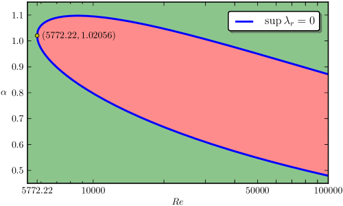
Figure 1: Neutral stability curve (in blue) for the laminar solution, using $n\lesssim 1000$ discretization points. For each pair $(Re,\alpha)$ in this curve, the most unstable eigenvalue $\lambda$ is purely imaginary. The curve splits the $Re$-$\alpha$ plane in two stability regions as shown in the graph: the green one is stable and the red one unstable.

IV Periodic solutions

IV.1 The Orr–Sommerfeld equation

Before applying the previously described numerical scheme, we make some considerations about the linearized stability of the laminar flow and time-periodic solutions. We start from the linearization of the vorticity equation around the basic flow, which is known as the Orr–Sommerfeld equation

$$(u_{b}-\frac{\lambda\mathrm{i}}{\alpha})(\phi^{\prime\prime}-\alpha^{2}\phi)-u_{b}^{\prime\prime}\phi=\frac{1}{\mathrm{i}\alpha Re}(\phi^{(4)}-2\alpha^{2}\phi^{\prime\prime}+\alpha^{4}\phi).$$ (13)

It is a fourth order ordinary differential equation on $\phi=\phi(y)$ as eigenfunction, with $\lambda$ as eigenvalue, and boundary conditions $\phi(\pm 1)=\phi^{\prime}(\pm 1)=0$. For each $Re$ and $\alpha$, (13) represents an eigenvalue problem on $\lambda$ and $\phi$. In this way if $\lambda=\lambda_{r}+\mathrm{i}\lambda_{i}$ is a complex eigenvalue with $\lambda_{r}>0$, then the laminar flow is unstable to infinitesimal disturbances according to the linear theory.

We have employed finite differences to approximate $\phi(y)$ and its derivatives in an uniform mesh $\bar{y}_{m}=2m/(n+1)-1\in[-1,1]$ for $m=0,\ldots,n+1$ and $n$ a sufficiently large positive integer. After substituting $\phi(\bar{y}_{m}),\ m=0,\ldots,n+1$ and the approximation to its derivatives in (13), we obtain an eigenvalue problem of finite dimension: $A\phi=cB\phi$, for $A,B$ matrices depending only on $Re,\alpha$, and $n$: $A$ is pentadiagonal and $B$ tridiagonal. We solve the eigenvalue problem (by means of the inverse power method with adapted shifts) in order to simply get the eigenvalue with the largest real part, that is to say, the most unstable one. Precision is improved through extrapolations on the mesh size $2/(n+1)$. We have obtained the known results reported by other authors, e.g. Orszag (1971), with an analogous accuracy. The neutral stability curve, where $\lambda_{r}=0$, is presented in figure 1. In this figure, each point in the $Re$–$\alpha$ plane represents a perturbation of the laminar solution whose stability is decided upon its position: green points are stable, red ones unstable and blue ones neutrally stable. We also observe the critical Reynolds number, $Re_{cr}=5772.22$ for $\alpha=1.02056$, so that if $Re<Re_{cr}$ the laminar solution is linearly stable for any value of $\alpha$. Likewise, for $\alpha\gtrsim 1.1$ the laminar flow is linearly stable for every $Re$.

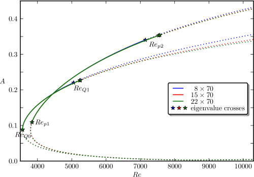
Figure 2: Bifurcating curve of periodic flows for several discretizations specified as $N\times M$, $\alpha=1.1$, and based on $Re_{p}$ and $Re_{Q}$. On each curve based on $Re_{p}$ there are several ‘*’ corresponding to Hopf bifurcations. They divide the different regions of stability to superharmonic disturbances, which are also represented in the plot as continuous (stable) and discontinuous (unstable) lines. In the $Re_{Q}$ case, the point labeled $Re_{Q0}$ represents a real eigenvalue crossing the imaginary axis, meanwhile $Re_{Q1}$ is a Hopf bifurcation. Likewise, at $Re_{Q0}$ it is attained the minimum $Re_{Q}$.

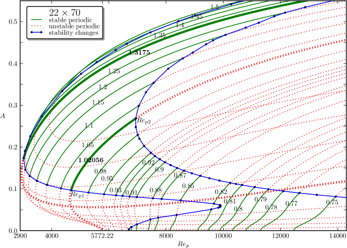
Figure 3: Bifurcating curves of periodic flows for $Re_{p}$ and several values of $\alpha$ specified on each curve. The number of discretization points is $N=22,M=70$. The ‘$\bullet$’ on each curve represents a change of stability. Joining those points we obtain $4$ regions: the corresponding solutions are unstable on the right and bottom-left regions and stable on the top region. In the intermediate region there are stable and unstable flows, even for a single $\alpha$, e.g. $\alpha=1.3175$. Curves for $\alpha=1.02056$ and $\alpha=1.3175$ are traced in thicker lines. For $\alpha=1.02056$ it is attained the critical Reynolds number at $Re_{p}=5772.22$ and for $\alpha=1.3175$ it is approximately reached a solution at a minimum $Re_{p}=2939$.

IV.2 Continuation of travelling waves

Next, we use the above results to look for periodic solutions in time. Due to the translational symmetry of the channel in the stream direction (artificial boundaries in (2)), it is showed in Rand (1982) that if we have $u(x,y,t)$ such that

$$u(x,y,t+T)=u(x,y,t),\quad\mbox{for all }x\in\mathbb{R},\quad y\in[-1,1],\quad t\geqslant 0$$

and some $T>0$ (that is, $u(x,y,t)$ is $T$-periodic in time), then it is a rotating (or travelling) wave, i.e.

$$u(x,y,t)=u(x-ct,y,0),\quad\mbox{for }c=\frac{L}{T}.$$ (14)

Consequently $u(x,y,t)$ is observed as a stationary solution in a system of reference moving at speed $c$ as it was introduced in (5). The converse is also true, namely every stationary solution of (5) gives rise to a time-periodic solution as is easily verified. This fact allows us to search for periodic solutions in time as functions $u(x,y)$ in a Galilean reference at speed $c$, which solve the stationary version of (5) or, in its discretized form, the stationary version of (10)

$$\begin{cases}0=U_{0}\\ 0=(I-P_{k}T_{k})^{-1}(\bar{U}_{k}-P_{k}\bar{V}_{k}),&k=1,\dots,N.\end{cases}$$ (15)

Given a fixed $\alpha$, what we have in (15) is a zeros search problem for a system of nonlinear equations of dimension $K$ (defined at the end of  ​§ III). It can be expressed as $H_{p}(Re,c,U)=0$. Solutions of (15) are locally unique for each $Re$, except translations in the stream direction. This is due to the fact that any translation of a rotating wave in the stream direction, gives rise to the same wave at a different time instant. Indeed, if $u(x,y,0)$ is the starting position of a rotating wave then, by (14), for every $\theta\in\mathbb{R}$ we have $u(x-\theta,y,0)=u(x,y,\theta/c),$ and thus $u(x-\theta,y,0)$ lies in the same orbit as $u(x,y,0)$. In order to achieve uniqueness, we fix one of the coordinates of $U$, by restricting it to a Poincaré section

$$\Sigma_{1}=\left\{U=(\bar{u}_{0},\dots,\bar{u}_{N})\ |\ \Re(\bar{u}_{11})=s_{1}\right\},$$ (16)

($\Re(u),\Im(u)$ stand for the real and imaginary part of $u$), for $s_{1}\in\mathbb{R}$, a fixed value. We mainly set $s_{1}=0$, since this choice gives well conditioned systems. If we fix $Re$ in (15), the number of unknowns, $K$, is the same as the number of equations. We look for its solutions by means of pseudo-Newton’s method, in which we factorize the resulting linear system using a direct $LU$ decomposition. The first approximation of the Jacobian matrix $DH_{p}$ is implemented by finite differences with extrapolation. Every column of this matrix is obtained evaluating $H_{p}$ in parallel in a Beowulf system. Subsequent updates of $DH_{p}$ are carried out by Broyden’s ‘good’ formula. As a consequence, at each pseudo-Newton step we only have to apply rank-one updates to the $LU$ factorization of $DH_{p}$. These improvements mean an enormous increase in the speed of computations.

If we use $Re$ as a continuation parameter, we can trace the one-parameter curve $H_{p}(Re,c,U)=0$. This is implemented numerically by pseudo-arclength continuation. To this end, we compute the unit-norm tangent vector to the curve. This vector and previously computed points on the curve, are used to predict the next solution point, which is finally corrected by pseudo-Newton iterations.

The starting point of those iterations is a numerically integrated periodic solution. We obtain it using the numerical integrator (12). The initial condition is taken as a small perturbation of the laminar flow. At the same time we check our previous results and those reported in Orszag (1971) about $Re_{cr}$. Namely, taking for example $\alpha=1.02056,Re>Re_{cr}$, we observe how the laminar flow is not stable, as it evolves to another steady flow which turns out to be $T$-periodic in time for some $T$. Up to errors of order $O((\Delta t)^{2})$ (those of the time discretization (12)), this $T$-periodic solution satisfies (15) and it is thus a rotating wave. We choose it as initial approximation to a point on the curve $H_{p}(Re,c,U)=0$.

Table 1: For some values of $\alpha$, this table shows the minimum values of $Re_{p}$ and $Re_{Q}$ for which exists periodic flow. Calculations made for $N=22$ and $M=70$. The minimum $Re$ attained is marked with ‘*’. Results are in good agreement with those reported by Herbert (1976) for $Re_{p}$.

$\alpha$	$\min Re_{Q}$	$\alpha$	$\min Re_{p}$
1.1000	3564.5164	1.1000	3797.0331
1.2236	2845.5884	1.2400	3048.0073
1.3000	2647.6068	1.3092	2939.3711
1.3424	2608.9990	1.3145	2939.2069
1.3520	2607.5519	1.3174	2939.0345
1.3521	$\phantom{\kern 4.26773ptl}2607.5516{}^{*}$	1.3175	$\phantom{\kern 4.26773ptl}2939.0343^{*}$
1.3523	2607.5520	1.3177	2939.0350
1.3534	2607.5753	1.3265	2940.6307
1.5000	3018.3031	1.4665	3526.0725

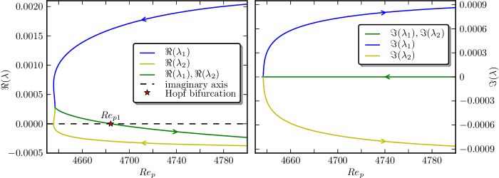
Figure 4: Real and imaginary part of the two most unstable eigenvalues ($\lambda_{1}$ and $\lambda_{2}$) of periodic flows for $N=22$, $M=70$, $\alpha=1.02056$ and $Re_{p}$ (cf. figure 3). Close to the minimum $Re_{p}$ of the amplitude curve, $\lambda_{1}$ and $\lambda_{2}$ are unstable and real, and give rise to a pair of complex conjugate eigenvalues. The first crossing through the imaginary axis is associated to a single real eigenvalue ($\lambda_{2}$), meanwhile the second one corresponds to the $Re_{p1}$ Hopf bifurcation ($\lambda_{1}$ and $\lambda_{2}$). Arrows for both graphs, point to the direction of increasing amplitude in figure 3.

Given a profile of velocities $(u,v)$ we define its amplitude $A$, as the distance to the laminar profile $(u_{b},0)$ in the $L^{2}$-norm

$$A=\frac{1}{2L}\|(u-u_{b},v)\|_{2},\qquad\|(u,v)\|_{2}^{2}=\int_{0}^{L}\int_{-1}^{1}\left[u(x,y)^{2}+v(x,y)^{2}\right]\mathrm{d}y\,\mathrm{d}x.$$ (17)

For a rotating wave as defined in (14), its amplitude does not depend on time since for fixed $t$:

$$\begin{array}[]{r@{}l}\displaystyle\int_{0}^{L}\int_{-1}^{1}u(x,y,t)^{2}\mathrm{d}y\,\mathrm{d}x\buildrel\mbox{\scriptsize 1}\over{=}&\displaystyle\int_{0}^{L}\int_{-1}^{1}u(x-ct,y,0)^{2}\mathrm{d}y\,\mathrm{d}x\\[12.91663pt] \displaystyle\buildrel\mbox{\scriptsize 2}\over{=}&\displaystyle\int_{-ct}^{L-ct}\int_{-1}^{1}u(\tilde{x},y,0)^{2}\mathrm{d}y\,\mathrm{d}\tilde{x}\buildrel\mbox{\scriptsize 3}\over{=}\int_{0}^{L}\int_{-1}^{1}u(\tilde{x},y,0)^{2}\mathrm{d}y\,\mathrm{d}\tilde{x}.\end{array}$$

In step 1 we apply definition (14). For step 2 we make the change of variable $\tilde{x}=x-ct$, and because $u$ is $L$-periodic in $x$ we have step 3.

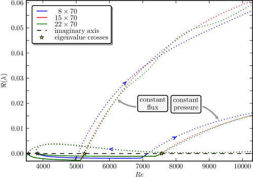
Figure 5: Real part of the most unstable eigenvalue for periodic flows for $\alpha=1.1$ and $N\times M$ as specified. For the $Re_{p}$ case, the two crossings of each curve with the imaginary axis corresponds to the first two ‘*’ of figure 2, and are detailed in table 2 as $Re_{p1}$ and $Re_{p2}$. In the analogous plot based on $Re_{Q}$, the two crossings of each curve with the imaginary axis corresponds to the first two ‘*’ of figure 2 and are also specified in table 2 as $Re_{Q0}$ and $Re_{Q1}$. Continuous and discontinuous lines refer respectively to stable and unstable periodic solutions associated to each point $(Re,\Re(\lambda))$. Arrows point to the direction of increasing amplitude in figure 2.

IV.3 Stability of periodic solutions

We notice that zeros of system (15) can either correspond to stable or unstable time-periodic solutions. With a stable solution it is meant the one for which any small disturbance ultimately decays to zero, whereas if some of those disturbances remain permanently away from zero, it is called unstable.

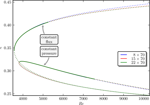
Figure 6: Speed of the observer $c$, for parameters and periodic solutions as in figure 2. On both $Re_{p}$ and $Re_{Q}$ cases, upper and lower branches correspond to the respective ones of amplitudes. Unlike $Re_{p}$, for the constant flux case the upper branch increases with $Re_{Q}$. Continuous and discontinuous lines refer respectively to stable and unstable periodic solutions associated to each $c$.

To decide whether a time-periodic flow $u$ is stable or not, we consider it as a steady solution for its appropriate $c=L/T$ and obtain the eigenvalues of its Jacobian matrix. This matrix is computed analytically linearizing (10) around $u$. If every eigenvalue has negative real part, the periodic flow is stable to disturbances of the same wavenumber $\alpha$ but, if there is an eigenvalue with positive real part, the solution is unstable. Let us mention that there is always a zero eigenvalue which corresponds to the lack of uniqueness of the time-periodic flow due to translations. Setting $\alpha=1.1$, the bifurcating diagram for the periodic flows in the $Re$-$A$ plane together with the stability changes are represented in figure 2 for both formulations in terms of $Re_{p}$ and $Re_{Q}$. Due to relations (3) and (4) we only need to compute travelling waves $u^{p}(x,y,t)$ at speed $c$ for $Re_{p}$, since (4) gives the associated $u^{Q}(x,y,t)$, which is easily checked to be a travelling wave at speed $rc$ for $Re_{Q}$, being $r=Re_{p}/Re_{Q}$. As well as computing the eigenvalues, we confirm the stability of a periodic flow using the numerical integrator (12). A more complete picture of the different connections among stable and unstable solutions is given in Casas and Jorba (2004).

By simply taking a known travelling wave for some $\alpha$ as initial guess and moving slightly $\alpha$, we can find periodic solutions for different values of $\alpha$. These are shown in figure 3, together with their stability. In addition, in table 1 we have computed, for several values of $\alpha$, the corresponding minimum value of $Re_{p}$ and $Re_{Q}$ (denoted as $Re_{min}(\alpha)$) along the amplitude curves (see figure 3). In turn, $Re_{min}(\alpha)$, is minimized as a function of $\alpha$. In this way we obtain the absolute minimum $Re_{p}$ and $Re_{Q}$ for which there exists periodic solution. These minimum values are marked with ‘*’ in table 1. For $Re_{p}$, Herbert (1976) obtained the minimum value at $Re_{p}=2934.80$ for $\alpha=1.3231$ and $N\times M=4\times 40$ as the spectral spatial discretization for the stream function: this discretization is analogous to the one used in the present work. We observe that our value of $Re_{p}$ differ from Herbert’s not more than $0.15\%$.

Previously, Soibelman and Meiron (1991) found similar bifurcations of travelling waves for $\alpha=1.1$, and the critical Reynolds number for which there are time-periodic solutions: $Re_{p}\approx 2900$ for $\alpha\approx 1.3$, and $Re_{Q}\approx 2600$. We remark that in figure 3 for $\alpha=1.3175$ there exists an attracting periodic solution for $Re_{p}=3024$ which corresponds to $Re_{Q}=2630$. For the case of the laminar flow, we encounter the classical results of Orszag (1971) about the critical Reynolds being at $Re_{cr}=5772.22$ for $\alpha=1.02056$. On the one hand, we observe in figure 3 that the bifurcation curve of periodic flows reaches the laminar solution at the above mentioned $Re_{cr}$ and in addition, the laminar solution is checked to be stable when $Re<Re_{cr}$ and unstable if $Re>Re_{cr}$. This Hopf bifurcation at $Re_{cr}$ is called subcritical, because the branch of periodic solutions emanating at it decreases in $Re$. When the new branch increases in $Re$, we call it supercritical bifurcation. We also notice that for $\alpha=1.02056$, it is reached the minimum Reynolds number where the transition from stable to unstable laminar flow takes place, what was formerly presented in figure 1. For $\alpha\gtrsim 1.1$ the curve of periodic solutions does not reach the laminar flow. This is in agreement with the situation shown in figure 1, since for $\alpha\gtrsim 1.1$ the laminar flow is linearly stable for every $Re$. In figure 3 we check as well that for $\alpha\gtrsim 0.91$ the curve of periodic flows bifurcates subcritically from the laminar flow, but for $\alpha\lesssim 0.91$ the Hopf bifurcation is changed into supercritical. Precisely for $\alpha\approx 0.915$ it is born a new change of stability on the curve of travelling waves at $Re_{p}\approx 6700$. The behaviour around this new point is saddle-node bifurcation, analogous to $Re_{Q0}$, and will be described in the following subsection.

Table 2: Minimum Reynolds number $Re_{Q0}$ and the three Hopf bifurcations of periodic flows at $Re_{p1}$, $Re_{Q1}$, $Re_{p2}$, together with associated parameters $c$ and $\tau$ for $\alpha=1.02056,1.1$, $M=70$ and several $N$. The values reported in Soibelman and Meiron (1991) for $M=70$ are also included.

$N$	$Re_{Q0}$	$c_{0}$	$Re_{p1}$	$c_{1}$	$\tau_{1}$	$Re_{Q1}$	$c_{1}$	$\tau_{1}$	$Re_{p2}$	$c_{2}$	$\tau_{2}$
Present work for $\alpha=1.02056$
4	4439.1	0.31544	4701.7	0.29729	9662.43	5620.0	0.37239	13.52	7450.1	0.28091	17.93
5	4387.1	0.31934	4684.6	0.29881	8983.08	5108.0	0.36054	14.00	6347.5	0.29014	17.39
6	4393.9	0.31890	4686.1	0.29868	9080.07	5085.8	0.36257	13.78	6355.4	0.29013	17.22
7	4396.3	0.31845	4684.1	0.29853	9143.27	5243.2	0.36468	13.68	6643.2	0.28783	17.33
8	4395.4	0.31854	4684.1	0.29857	9125.21	5335.6	0.36610	13.67	6827.8	0.28608	17.49
9	4395.2	0.31858	4684.3	0.29858	9120.06	5341.9	0.36637	13.70	6845.0	0.28592	17.55
10	4395.2	0.31857	4684.2	0.29858	9120.76	5353.9	0.36653	13.68	6865.9	0.28581	17.54
11	4395.2	0.31858	4684.2	0.29858	9120.24	5371.9	0.36680	13.64	6900.7	0.28555	17.52
12	4395.2	0.31858	4684.2	0.29858	9119.98	5385.0	0.36703	13.62	6926.8	0.28534	17.52
⋮						⋮	⋮	⋮	⋮	⋮	⋮
18						5253.3	0.40634	11.78	6936.0	0.28530	17.51
19						5389.8	0.36711	13.61	6934.9	0.28532	17.51
20						5390.4	0.36713	13.61	6936.3	0.28530	17.51
21						5390.3	0.36712	13.61	6935.9	0.28531	17.51
22						5390.3	0.36712	13.61	6936.1	0.28531	17.51
Present work for $\alpha=1.1$
4	3603.5	0.34248	3864.5	0.31927	7429.40	5812.6	0.41532	11.62	8946.1	0.26985	17.88
5	3564.7	0.34467	3841.0	0.32004	7090.00	5296.6	0.40633	11.65	7670.3	0.28059	16.87
6	3562.8	0.34506	3841.4	0.32018	7065.52	4840.4	0.40235	11.93	6732.7	0.28927	16.59
7	3564.9	0.34475	3840.8	0.32010	7100.29	4905.9	0.40270	11.88	6844.8	0.28863	16.58
8	3564.7	0.34474	3840.6	0.32010	7098.78	5054.0	0.40392	11.85	7145.8	0.28568	16.75
9	3564.5	0.34477	3840.6	0.32010	7096.05	5107.8	0.40457	11.86	7264.9	0.28445	16.87
10	3564.5	0.34477	3840.6	0.32011	7095.79	5120.9	0.40477	11.87	7292.5	0.28424	16.90
11	3564.5	0.34477	3840.6	0.32011	7095.68	5157.2	0.40519	11.84	7368.9	0.28358	16.92
12	3564.5	0.34477	3840.6	0.32011	7095.56	5189.1	0.40555	11.82	7436.6	0.28298	16.94
⋮						⋮	⋮	⋮	⋮	⋮	⋮
21						5246.8	0.40624	11.78	7558.9	0.28197	16.97
22						5250.4	0.40629	11.78	7567.0	0.28190	16.98
23						5249.5	0.40628	11.78	7565.0	0.28192	16.97
24						5250.6	0.40630	11.78	7567.4	0.28190	16.98
25						5249.6	0.40628	11.78	7565.2	0.28192	16.98
Soibelman and Meiron (1991) for $\alpha=1.1$
2			3630		4742.32	5600		20.6	9400		35.50
3			3800		4935.43	6250		12.5	9675		17.65
4			3775		4875.63	5875		13.4	9592		16.54

IV.4 Hopf bifurcations

Now let us discuss the bifurcation diagram shown in figure 3 for $\alpha=1.02056$. First, the laminar solution becomes unstable at the critical value $Re_{cr}=5772.22$, due to a Hopf bifurcation that gives rise to a unstable family of periodic orbits. This family continues backwards (with respect to $Re$, i.e. it is subcritical) until $Re_{p}\approx 4636$, where a turning point is reached and $\Re(\lambda_{2})$ (described in figure 4) crosses the imaginary axis. Before arriving at this turning point, there is a single eigenvalue, $\lambda_{1}$, on the real positive axis, while the remaining ones have negative real part (we ignore the eigenvalue at $0$ arising from the lack of uniqueness of periodic flows). On traversing through the turning point, a real and negative eigenvalue ($\lambda_{2}$) becomes real positive, so the number of unstable eigenvalues is now two. Shortly after that, these two unstable eigenvalues collide and become a conjugate complex pair (still with positive real part), and then they cross the imaginary axis for $Re_{p}\approx 4684$ producing a new Hopf bifurcation at the point $Re_{p1}$ on figure 3. Between $Re_{p1}$ and $Re_{p2}\approx 6936$, the family of periodic orbits is stable to disturbances of the same wavelength. At $Re_{p2}$, there is another Hopf bifurcation produced by a pair of conjugate eigenvalues crossing the imaginary axis. These bifurcations persist, as shown in table 2, when $M,N$ are increased and no new ones seem to appear in this range.

The case of constant flux is qualitatively different. For $Re_{Q}$ the bifurcating diagram of periodic solutions has a turning point at a minimum value of $Re_{Q}$, which we designate as $Re_{Q0}$ (cf. figure 2). The lower branch of periodic solutions is unstable with only one unstable real eigenvalue and the upper is initially stable, being also real the most unstable eigenvalue. On traversing the bifurcating curve towards the upper branch, this real positive eigenvalue becomes negative at the turning point. The upper branch is kept stable until a subsequent Hopf bifurcation appears at certain value $Re_{Q1}$. For $Re_{Q}\gtrsim 7000$ and $\alpha=1.1$, we have detected more Hopf bifurcations which we do not consider in this study. However for the range included in figure 2 all periodic flows for $Re_{Q}>Re_{Q1}$ are unstable.

Pugh and Saffman (1988) pointed out that the null eigenvalue at $Re_{Q0}$ has algebraic multiplicity $2$ and geometric multiplicity $1$. We can consider that eigenvalue simple (with algebraic and geometric multiplicity 1) if we ignore the constant zero eigenvalue due to a trivial phase shift of the flow in the stream direction. The suppression of this trivial null eigenvalue can be made by restricting equations (10) to the closed linear manifold $\Sigma_{1}$ defined as a Poincaré section in (16). According to bifurcation theory, at a simple eigenvalue like this one we have no equilibrium point for $Re_{Q}<Re_{Q0}$ and two equilibrium points for $Re_{Q}>Re_{Q0}$: this situation corresponds to a saddle-node bifurcation and no new branches of solutions come out from $Re_{Q0}$.

In table 2 are shown $Re_{p}$, $Re_{Q}$, the speed of the observer $c$ and the period $\tau$ of the bifurcated solution corresponding to the first Hopf bifurcations for several values of $N$ and $M=70$. Taking $M=70$, Chebyshev modes seem to be enough to attain convergence in the results. The values obtained by Soibelman and Meiron (1991) are also presented for comparison. For $\alpha=1.1$ we observe convergence of our results on the different Hopf bifurcations considered as $N$ is increased. In all cases there are substantial differences with Soibelman and Meiron’s Soibelman and Meiron (1991) results, being in more agreement for the lowest $Re$. We remark the slow convergence of the Fourier series to the bifurcation values as $N$ is increased. At the same time we have also obtained convergence in the qualitative behaviour: the subcritical or supercritical character of all the studied Hopf bifurcations remain unaltered as $M,N$ are increased.

Formulas (3) and (4) provide again the correspondence between bifurcation points at $Re_{Q}$ and $Re_{p}$ (cf. table 2). For instance at $Re_{p1}=3840.6$ for $N=12$, $M=70$ and $\alpha=1.1$, the periodic solution transformed by these formulas furnish a periodic solution at $Re_{Q}=3564.5$ and $c=0.34490$, values in good agreement with $Re_{Q0}$ reported in table 2. Likewise, the transformed periodic solution for $N=25$, $\alpha=1.1$ at $Re_{Q1}=5249.6$ gives rise to $Re_{p}=7565.5$ and $c=0.28192$, again in good precision with respect to $Re_{p2}$.

The different stability changes marked as a blue dot in figure 3, roughly divide the $Re_{p}$-$A$ plane in four regions. On the right and bottom-left regions the corresponding periodic solutions are unstable (filled with red points), meanwhile they are stable on the top region (only green points). In the intermediate region there are both stable and unstable flows, even for a single $\alpha$, e.g. $\alpha=1.3175$. Through this classification, given a periodic flow with its associated $(Re_{p},A)$, we can deduce its stability, independently on $\alpha$ in some cases. On traversing the $Re_{p1}$ blue curve in the direction of increasing amplitudes, up to the relative maximum on that curve attained at $Re_{p1}\approx 9909$ for $\alpha\approx 0.814$, we encounter saddle-node bifurcations for $\alpha\in[0.88,0.915]$ at a relative maximum on each bifurcation curve. For $\alpha\in[0.714,0.88]$, the former relative maximum disappears and the saddle-node bifurcation turns into a Hopf one. The rest of the $Re_{p1}$ curve is made up of Hopf bifurcations for the studied values $\alpha\leqslant 1.7$. The minimum $Re_{p1}\approx 3024$ is reached precisely for $\alpha\approx 1.3175$, where the minimum periodic flow was found in  ​§ IV.3. The $Re_{p2}$ blue curve is only constituted of Hopf bifurcations for the $\alpha\in[0.74,1.3175]$ considered. The minimum $Re_{p2}\approx 6936$ is achieved again for the critical $\alpha\approx 1.02056$.

The maximum growth rate (real part of the most unstable eigenvalue) for each periodic flow is presented in figure 5 for the same parameters as in figure 2. For the most unstable eigenvalue $\lambda$, $\Re(\lambda)$ crosses the imaginary axis twice, on the values $Re_{p1}$ and $Re_{p2}$ for $Re_{p}$ and on $Re_{Q0}$ and $Re_{Q1}$ for $Re_{Q}$. Those diagrams represent the degree of instability of each flow. Comparing to figure 2, we observe that at the same $Re$ on the upper branch of amplitudes, periodic solutions based on $Re_{Q}$ are more unstable than the associated ones based on $Re_{p}$. On the other hand, on the lower branch of amplitudes, at the same $Re$, both curves of $\Re(\lambda)$ visually coincides for $Re\gtrsim 5000$. This behaviour is also reflected in figures 2 and 6. In this last figure we present qualitatively different curves for the speed $c$ in $Re_{p}$ and $Re_{Q}$ cases. In the first case. $c$ is decreasing in both branches of solutions in figure 2. However, for $Re_{Q}$ the shape of the $c$-curve is similar as the $A$-curve in figure 2.

V Quasi-periodic solutions

In this section, we study the quasi-periodic flows that appear at the Hopf bifurcations of rotating waves shown in  ​§ IV. They are found as time-periodic orbits in an appropriate Galilean reference, which simplifies enormously their search. Those time-periodic orbits are obtained as fixed points of a Poincaré section, by means of a pseudo-Newton method. We have traversed bifurcating branches of quasi-periodic solutions for the Hopf bifurcations at $Re_{p1}$, $Re_{p2}$ and $Re_{Q1}$ defined in  ​§ IV. We have obtained different qualitative results than the ones reported in Soibelman and Meiron (1991). For $\alpha=1.1$ and $Re_{p}$ they found that the bifurcation at $Re_{p1}$ to quasi-periodic solutions is subcritical: they obtained quasi-periodic solutions for $Re_{p}$ before the bifurcation point. In consequence, close to that point, those bifurcated flows are stable. In the present study, by increasing the number of Fourier modes $N$, we have achieved a supercritical Hopf bifurcation at $Re_{p1}$: the bifurcating quasi-periodic flows are located for $Re_{p}$ after the bifurcation point and therefore close to it they are unstable. This is treated in  ​§ V.2. For the second Hopf bifurcation at $Re_{p2}$, in agreement with Soibelman and Meiron (1991), the quasi-periodic orbits are found for $Re_{p}$ greater than the bifurcation point. More details are given in  ​§ V.3. The behaviour at $Re_{Q1}$ (considered in  ​§ V.4) is analogous to that of $Re_{p2}$. However for $Re_{Q}>Re_{Q1}$ large enough we have detected another Hopf bifurcation to tori with $3$ basic frequencies. The stability of quasi-periodic flows to superharmonic disturbances is estimated by means of the linear part of the Poincaré map and also with a full numerical simulation of the fluid.

V.1 Reduction to periodic and numerical procedures

We use again the spatio-temporal symmetry of our system, due to the artificial boundaries of the channel. Considering this symmetry in Rand (1982) it is proved that every solution $u(x,y,t)$ that lies on an isolated invariant $2$-torus (a quasi-periodic solution), not asymptotic to a rotating wave, is a modulated wave, that is to say, there exists $\tau>0$ and $\phi\in\mathbb{R}$ such that

$$u(x,y,n\tau+t)=u(x-n\phi,y,t)\quad\mbox{for every }n\in\mathbb{Z}.$$ (18)

Hence, this kind of wave has the property that, may be viewed as a $\tau$-periodic wave in time, in a frame of reference moving at speed $c=(pL+\phi)/\tau$, for any integer $p$. In effect, defining $\tilde{x}=x-ct$ for that value of $c$, and $\tilde{u}(\tilde{x},y,t)=u(\tilde{x}+ct,y,t)$ as the velocity in the moving frame of reference at speed $c$, it turns out that

$$\tilde{u}(\tilde{x},y,\tau)\buildrel\mbox{\scriptsize 1}\over{=}u(\tilde{x}+c\tau,y,\tau)\buildrel\mbox{\scriptsize 2}\over{=}u(\tilde{x}+pL+\phi,y,\tau)\buildrel\mbox{\scriptsize 3}\over{=}u(\tilde{x},y,0)\buildrel\mbox{\scriptsize 4}\over{=}\tilde{u}(\tilde{x},y,0).$$ (19)

In steps 1, 4 we use the previous definition of $\tilde{u}$. Substituting the previously defined $c$ we obtain step 2, and because $u$ is $L$-periodic in $x$ and a modulated wave, one gets step 3. Consequently we have proved that $\tilde{u}(\tilde{x},y,t)$ is a $\tau$-periodic function of $t$.

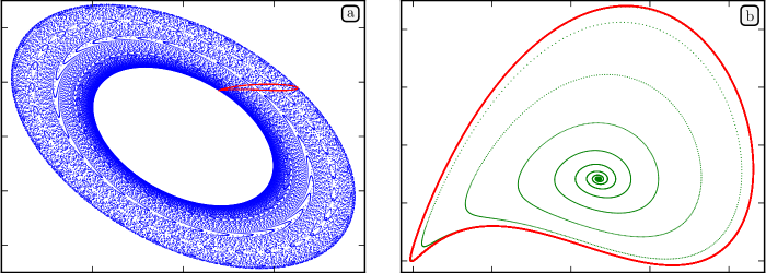
Figure 7: Two representations of the solution vector $U(t)$ of a quasi-periodic flow projected on the plane of two selected coordinates namely, $M-1+(2N-3)(M-2)+3$, and $M-1+2(M-2)+5$, for $Re_{p}=3865,\alpha=1.1,N=8,M=70$. The range of values for (a) is $[-0.002,0.002]\times[-0.001,0.001]$ and $[0.00037,0.00129]\times[0.000338,0.000385]$ for (b). In (a) a dot is plotted each $\Delta t=0.02$ time units, meanwhile in (b) only for $t$ such that $U(t)\in\Sigma_{1}$. The red closed curve in (b) is obtained integrating repeatedly for $t\in[0,\tau]$. This curve is also represented as a reference on the right centre of (a).

In order to look for periodic flows satisfying (19) in a Galilean reference at speed $c$, we make use of the Poincaré section $\Sigma_{1}$ defined in (16). In this case, we only consider points on $\Sigma_{1}$ when they cross the section in a particular direction as time increases, namely, from $s_{1}<0$ to $s_{1}>0$. Likewise we define the associated Poincaré map $P_{c}:\Sigma_{1}\longrightarrow\Sigma_{1}$ as follows: starting from an initial condition $U=U(0)\in\Sigma_{1}$ we integrate (10) for fixed parameters $Re$, $\alpha$ and $c$, until a time $t_{c}$ such that $\smash{\tilde{U}(t_{c})}\in\Sigma_{1}$ ($\smash{\tilde{U}(t_{c})}$ represents the evolution of $U(0)$ in a Galilean reference at speed $c$) for the $n_{c}$-th time (i.e. after $n_{c}$ crosses with $\Sigma_{1}$), where $n_{c}$ is a positive integer which represents the minimum number of times needed for the flow to return close to the initial point $U(0)$ (the meaning of ‘close’ will be specified in  ​§ V.2). We then set $P_{c}(U(0))=\smash{\tilde{U}(t_{c})}$. In this way we have reduced the search of quasi-periodic flows to a zeros finding problem for the map $H_{q}$ defined as

$$0=H_{q}(Re,c,U)\buildrel\mbox{\scriptsize def}\over{=}P_{c}(U)-U=\tilde{U}(t_{c})-U(0).$$ (20)

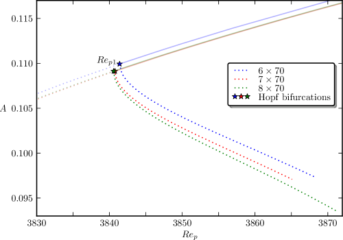
Figure 8: Bifurcated branches of quasi-periodic flows at the supercritical Hopf bifurcation of periodic flows at $Re_{p1}$. Each curve represents $A$ as a function of $Re_{p}$ and has specified $N\times M$. Both branches of periodic (in lighter colors) and quasi-periodic flows are presented. Calculations are shown for $\alpha=1.1$ and $\Delta t=0.02$. The ‘*’ correspond to the Hopf bifurcation at $Re_{p1}$ presented in figure 2. For the range shown, the bifurcating branch consists of unstable quasi-periodic orbits (dotted lines), whose amplitude decreases with $Re_{p}$.

From (18) we have that, if $P_{c}(U(0))=\tilde{U}(\tau)=U(0)$, for some $\tau$, then as well $P_{c}(V(0))=\tilde{V}(\tau)=V(0)$ for $V(0)=P_{0}^{k}(U(0))$ and $k$ any positive integer. Indeed, we can express (19) as $\tilde{u}(\tilde{x},y,\tau+t_{1})=\tilde{u}(\tilde{x},y,t_{1})$ for every $t_{1}$. From here, since $V(0)=U(t_{1})$ for some $t_{1}$, we immediately obtain $P_{c}(V(0))=V(\tau)=V(0)$. Therefore we can generate different points on the same orbit as a solution of (20). We avoid this lack of uniqueness by restricting $P_{c}:\Sigma_{1}\cap\Sigma_{2}\longrightarrow\Sigma_{1}$, for $\Sigma_{2}$ a Poincaré section (analogous to $\Sigma_{1}$) defined by

$$\Sigma_{2}=\left\{U=(\bar{u}_{0},\dots,\bar{u}_{N})\ |\ S=0\right\},$$ (21)

where we set $S=\Re(\bar{u}_{N,M/2-1})-s_{2}$, for $s_{2}\in\mathbb{R}$ a suitable quantity. For $Re$ close to the studied Hopf bifurcations, we have chosen $s_{2}=\Re(\bar{u}^{p}_{N,M/2-1})$, with $u^{p}\in\Sigma_{1}$ the travelling wave at the exact $Re$ where the bifurcation takes place. The reason for this choice is merely to preserve continuity in the amplitude diagrams described next.

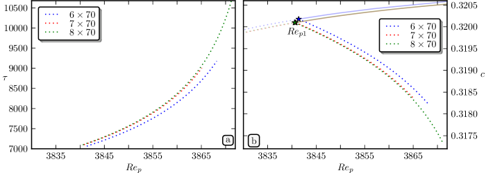
Figure 9: Different curves related to figure 8 for $N\times M$ points as specified. (a) $\tau$ represents the period in time for a quasi-periodic flow when the observer sees it as periodic. (b) The appropriate value of $c$ that converts a quasi-periodic flow in periodic, together with the corresponding curve for periodic flows in lighter colors (cf. figure 6). The ‘*’ correspond to the Hopf bifurcations at $Re_{p1}$ presented in figure 2.

In order to trace the curve $H_{q}(Re,c,U)=0$, we utilize the same continuation method as for system $H_{p}(Re,c,U)=0$ in (15), differing essentially in the definition of the equation to vanish: for periodic flows the computations are much simpler and faster than for quasi-periodic ones. The solution of (20) needs an initial guess, which is obtained as described in the following subsections. Once we have a quasi-periodic flow such that $H_{q}(Re,c,U)=0$, we measure its amplitude $A$, as in the case of periodic flows (cf. (17)). If $u(x,y,t)$ is a modulated wave, using (18) and the $L$-periodicity we have

$$\int_{0}^{L}\int_{-1}^{1}u(x,y,\tau)^{2}\,\mathrm{d}y\,\mathrm{d}x=\int_{0}^{L}\int_{-1}^{1}u(x-\phi,y,0)^{2}\,\mathrm{d}y\,\mathrm{d}x=\int_{0}^{L}\int_{-1}^{1}u(x,y,0)^{2}\,\mathrm{d}y\,\mathrm{d}x.$$ (22)

Since we have numerically checked that $A$ is not constant for modulated waves, we conclude from (22) that it is a $\tau$-periodic function of $t$. This is not so for the rotating waves of  ​§ IV, for which $A$ is constant in time. In the case of a quasi-periodic flow $U(t)$, with the purpose of considering a concrete value for the amplitude, we evaluate $A(t)$, at $t$ such that $U(t)\in\Sigma_{1}\cap\Sigma_{2}$. This is simply a representative and easy to compute value for $A(t)$, as we cannot obtain a single value for the amplitude of this class of flows. We use it to trace the continuation curve: it provides the distance to the laminar solution at some time instant. In the same way, $c$ can be considered as a representative and time independent value for every quasi-periodic flow, so that we can as well use it to trace continuation curves.

V.2 Hopf bifurcation at $Re_{p1}$

For $Re_{p}<Re_{p1}$ and $\alpha\approx 1$ the corresponding time-periodic flow in figure 3 is unstable, but its temporal evolution ultimately decays to the laminar flow. The results in Soibelman and Meiron (1991) point out the existence of a subcritical Hopf bifurcation at $Re_{p1}$: they use the vorticity equation and only consider $N\leqslant 2$ Fourier modes. According to bifurcation theory (see Marsden and McCracken (1976)), this means that the bifurcating quasi-periodic flows are locally stable. Following this result we tried to find quasi-periodic flows in the subcritical region, but with no success: we were not able to detect a quasi-periodic attracting solution for $Re_{p}<Re_{p1}$ and $N\geqslant 3$. In consequence we direct the search of quasi-periodic flows to the supercritical region, i.e. for $Re_{p}>Re_{p1}$.

It is also known from bifurcation theory that, in the case of a supercritical Hopf bifurcation in which fixed points before it are unstable and after it stable, the branch of periodic solutions that emanates at the bifurcation point is locally unstable. That should be the situation for $Re_{p}>Re_{p1}$ and thus the bifurcating quasi-periodic flows are locally unstable and therefore hard to locate by direct numerical integration, because the evolution of the fluid close to them does not remains near as time evolves.

On the other hand, pseudo-Newton’s method applied to solve (20) does not distinguish between stable or unstable flows. However, the difficult task is the search of a good starting guess for (20); it is carried out as follows. First we consider an unstable time-periodic solution $U^{p}_{1}(t)$, i.e. a fixed point of (10), for certain $Re_{1}<Re_{p1}$. Close to the Hopf bifurcation $Re_{p1}$ in the unstable region $Re_{p}<Re_{p1}$, the linearization of (10) around $U^{p}_{1}$ has just a couple of complex conjugate eigenvalues, $\lambda=\lambda_{r}\pm i\lambda_{i}$ with $\lambda_{r}>0$ (cf.  ​§ IV). If $w=w_{r}\pm iw_{i}$ is the associated eigenvector, we choose $v\in\langle w_{r},w_{i}\rangle$, i.e. $v$ is in the plane of the most unstable directions, along which the flow escapes in the fastest fashion from $U^{p}_{1}$. Now we change to $Re_{2}>Re_{p1}$ close to the bifurcation and select $c_{2}$ near to the one associated with the corresponding periodic orbit $U^{p}_{2}$ at $Re_{2}$, i.e. $H_{p}(Re_{2},c_{2},U^{p}_{2})=0$. For $Re_{2},c_{2}$ and $|r|\ll 1$ a small constant, we integrate numerically the initial condition $U=U^{p}_{1}+rv$, until a time when it become as closest as possible to a solution of $H_{q}(Re_{2},c_{2},U)=0$. This first approximation of $c_{2}$ is optimized by using minimization algorithms. In this case we also observe a value $\tau$ of the return time of $P_{c}$, neighbouring to $2\pi/|\mbox{Im}(\lambda)|$, taking $\lambda$ as the unique purely imaginary eigenvalue (together with its conjugate) at the Hopf bifurcation $Re_{p1}$.

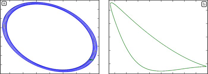
Figure 10: Two representations of the solution vector $U(t)$ of an (almost resonant) quasi-periodic flow projected on the plane of the same coordinates as figure 7, for $Re_{p}=7000,\alpha=1.02056,N=22,M=70$. The range of values for (a) is $[-0.00185,0.00185]\times[-0.004,0.004]$ and $[0.00147,0.00164]\times[-0.002495,-0.002385]$ for (b). In (a) a dot is plotted each $\Delta t=0.01$ time units. In (b) a dot is plotted only for $t$ such that $U(t)\in\Sigma_{1}$. The curve in (b) is also represented as a reference on the lower right corner of (a) as a small green line.

The initial guess obtained in this way is improved through pseudo-Newton’s iterations applied to the function $H_{q}$, to finally obtain a first unstable modulated wave for $Re_{p}>Re_{p1}$. In figure 7 we present numerical evidence that solutions $U(t)$ of (20) lie in a $2$-torus and are unstable in time for supercritical $Re_{p}$. In a) we observe how the trajectory, projected on a plane of two arbitrary coordinates of $U(t)$, fills densely a $2$-torus. On the outer red curve of b), it is simply plotted $U(t)$ when $U(t)\in\Sigma_{1}$ with the following adaptation: if $t>\tau$, being $\tau$ the period of $U(t)$ as a modulated wave, we plot $U(s)$ for $s$ such that $0\leqslant s=t-p\tau<\tau$ and $p=[t/\tau]$, ($[\cdot]$ stands for the integer part) i.e. we treat $U(t)$ as if it were exactly $\tau$-periodic in order to avoid its unstability. We note that, as we are on the Poincaré section $\Sigma_{1}$, the $2$-torus in a) is reduced to a closed curve in b), which corresponds to the unstable quasi-periodic flow, seen as if it were unperturbed by numerical errors. Likewise in b) we let the flow evolve for long time and plot again $U(t)$ (in green) when $U(t)\in\Sigma_{1}$ but suppressing the previous time adaptation. Here we can check that the flow is unstable, because it moves away from the outer closed curve and falls to the time-periodic and stable régime: a simple point in the centre of the figure.

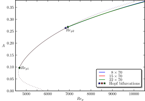
Figure 11: Bifurcated branches of quasi-periodic flows at the supercritical Hopf bifurcation of periodic flows at $Re_{p2}$. Each curve represents $A$ as a function of $Re_{p}$ and has specified $N\times M$. Both branches of periodic (in lighter colors) and quasi-periodic flows are presented (the green color almost completely conceals the red one). Calculations are shown for $\alpha=1.02056$ and $\Delta t=0.02$. The ‘*’ correspond to the $Re_{p1},Re_{p2}$ Hopf bifurcations presented in figure 3. For the range shown, the bifurcating branch consist of quasi-periodic orbits, stable to disturbances of the same wavenumber.

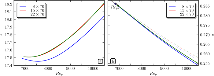
Figure 12: Different curves related to figure 11 using $Re_{p}$ in the abscissa axis for $N\times M$ points as specified. (a) and (b) are as in figure 9. In (b), in lighter colors, it is also drawn the periodic flows around $Re_{p2}$ (marked with ‘*’). In this case, the green color almost completely conceals the red one.

Once we have obtained the first solution of (20) by the pseudo-Newton’s method, we use continuation methods to traverse the bifurcating branch of quasi-periodic flows parametrized by $Re_{p}$. In figure 8 we plot the amplitude $A$ for each quasi-periodic solution as a function of $Re_{p}$. It seems that we have achieved both qualitative and quantitative convergence because we obtain a similar graph in increasing the values of $N,M$. It looks also clear from this plot that the Hopf bifurcation is supercritical so, at least locally, solutions on the bifurcating branch are unstable. The analysis of the stability of a quasi-periodic solution is done by means of the eigenvalues of the linear part of $P_{c}$ at a fixed point $U(t)$ such that $P_{c}(U(0))=U(0)$. This computation, analogously to the matrix $DH_{q}$, is obtained by extrapolated finite differences. In the range of $Re_{p}$ presented in figure 8, the quasi-periodic solutions are unstable. Furthermore, unlike the bifurcation at $Re_{p2}$, solutions at $Re_{p1}$ present certain symmetry: $\hat{u}_{k}(y,t)$ (defined in  ​§ III) is an even or odd function of $y$ according to the parity of $k$.

We also observe in figure 9(a) for different values of $N$, an indicator of the numerical effort involved in the evaluation of the map $P_{c}$. The big slope of the $Re_{p}$-$\tau$ curve shows the high computational cost involved as $Re_{p}$ is slightly increased. For $Re_{p}\in[3840,3872]$, $\alpha=1.1$ and $\Delta t=0.02$ the time needed to return to $\Sigma_{1}$ is $\tau\in[7000,10700]$. Likewise it has been necessary to adapt dynamically the minimum number of times, $n_{c}$ (defined just before system (20)), that the solution crosses $\Sigma_{1}$ before it returns to the starting point. For $Re_{p}$ close to $Re_{p1}$, $n_{c}$ starts at $1$ and it is incremented by $1$ when $Re_{p}$ varies approximately in just $2$–$3$ units. The way we modify $n_{c}$ is described next. If we change slightly $Re_{p}$ the return time $\tau$ should be varied in accordance. Thus, we impose that the new value obtained for $\tau$ satisfy $|\tau-\tau_{o}|<\varepsilon$, for some tolerance $\varepsilon$ and $\tau_{o}$ the former return time. If this condition is not fulfilled we increase or decrease $n_{c}$ by one unit, until it is satisfied, or we decrease $Re_{p}$ if necessary.

In figure 9(b) is represented $c$ for the same range of $Re_{p}$. We observe for $c$, nearby values as their counterpart periodic flows (cf. figure 6), but in this case the curve has a large decreasing slope. We emphasize that the $c$ graph shows a bifurcation diagram of periodic and quasi-periodic flows, which is time independent in contrast to the $Re$-$A$ plot in figure 8.

V.3 Bifurcation at $Re_{p2}$

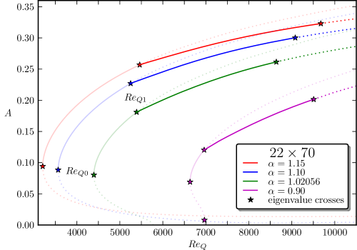
Figure 13: Analogous to figure 11 based on $Re_{Q1}$, using the specified $\alpha$ and $N\times M=22\times 70$, $\Delta t=0.01$. The bifurcated branches of quasi-periodic solutions have a change of stability at another Hopf bifurcation. Continuous and discontinuous lines represent stable and unstable flows respectively.

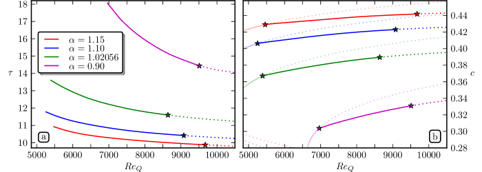
Figure 14: Values of $\tau$ (a) and $c$ (b) associated to quasi-periodic flows of figure 13. In (b), in lighter colors, it is also drawn the periodic flows around $Re_{Q1}$ of figure 13. Colors for curves in (a) are also valid for (b).

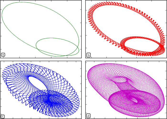
Figure 15: (a) An stable $2$-torus on $\Sigma_{1}$ for $Re_{Q}=8635$, $\alpha=1.02056$, $N\times M=22\times 70$, $\Delta t=0.009$. The integration time on the figure is about $1{,}222{,}000$ time units. (b) Analog of (a) for $Re_{Q}=8640$. We observe in this case that the initial $2$-torus is unstable and is attracted by a $3$-torus. The integration time on the figure is about $419{,}000$ time units. (c) The same as (b), but the initial condition is an unstable $2$-torus for $Re_{Q}=9750$ which is also attracted by a $3$-torus. The integration time is about $1{,}005{,}000$ time units. (d) The initial condition is an unstable $2$-torus for $Re_{Q}=10500$ and $\alpha=1.10$ which is again attracted by a $3$-torus. The integration time is about $1{,}002{,}000$ time units. The respective ranges in the four figures are $[0.0019,0.00445]\times[-0.00965,-0.0053]$, $[0.0018,0.0045]\times[-0.0098,-0.0052]$, $[0.0013,0.0058]\times[-0.0126,-0.005]$ and $[0.0016,0.00535]\times[-0.0147,-0.0078]$.

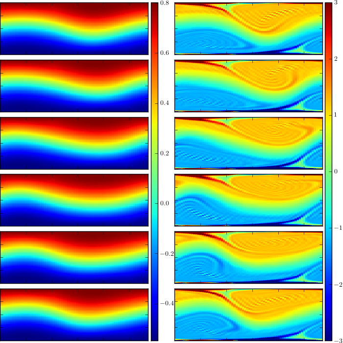
Figure 16: Stream lines (left) and levels of vorticity (right) for a unstable quasi-periodic flow at $Re_{Q}=10500,\alpha=1.1,N=22,M=70,\Delta t=0.009$. Surface levels are plotted for $0\leqslant x\leqslant L,-1\leqslant y\leqslant 1$. The depicted time instants from top to down are $0,\tau/6,2\tau/6,3\tau/6,4\tau/6$, and $5\tau/6$ for the associated orbit period $\tau=10.24$. Ranges for levels of stream lines and vorticity are $[-0.55,0.80]$ and $[-3,3]$ respectively. They are represented by a common scale of colors to the right of each column.

As we presented in figure 3, for $Re>Re_{p2}$ the corresponding periodic flow is unstable, so the evolution of (10) from such a flow as initial condition, drives the fluid away from it. By following the temporal evolution of this flow, we observe that the fluid seems to fall in a regular régime, which finally proves to be a quasi-periodic attracting solution. This is checked in figure 10 where we plot the projection of the solution vector $U(t)$ over the plane of the same two coordinates as in figure 7. Each point in figure 10(a) corresponds to the value of the specified coordinates at a time instant. As we can observe, the trajectory appears to fill densely the projection of a $2$-torus. Plotting the same coordinates as above, but only when $U(t)\in\Sigma_{1}$, we see in figure 10(b) a closed curve, which seems again to confirm that the flow lives in a $2$-torus.

Let us denote as $U^{0}(t)=(\bar{u}_{0}^{0},\dots,\bar{u}_{N}^{0})(t)$, a time instant of the flow in the attracting $2$-torus. We need to approximate the value of $c^{0}$ which better makes $U^{0}$ appear as a periodic flow. That $c^{0}$ exists according to (18)–(19). It can be estimated as (cf. Rand (1982))

$$c^{0}=\frac{2\pi}{k}\lim_{t\rightarrow\infty}\frac{n(t)}{t},\quad\mbox{for}\quad n(t)=\left[\frac{\arg(\mbox{Conj}{(\bar{u}^{0}_{km}(t))})}{2\pi}\right],$$

where $k$ is the number of peaks of the wave $U^{0}$ for $x\in[0,L]$ and we have used the midpoint of the channel for $m=M/2$. With $t$ large enough, $2\pi n(t)/kt$ gives an approximation of $c^{0}$ which we optimize using minimization. Next we use $U^{0},c^{0}$ as the initial condition for pseudo-Newton’s method applied to (20) to confirm that our attracting 2-torus $U^{0}$ is in fact a modulated wave. For a fixed $\alpha$, once we have a first point $(Re_{p},c^{0},U^{0})$ which satisfies (20), taking $Re_{p}$ as a continuation parameter, we can trace the curve of quasi-periodic flows in the $Re$–$A$ plane by pseudo-arclength numerical continuation, applied to $H_{q}$ as in  ​§ V.2.

As we observe in figure 11, there appears a branch of quasi-periodic solutions which bifurcates supercritically from the curve of periodic flows. We may again have zeros of $H_{q}(Re,c,U)$ that can either correspond to stable or unstable quasi-periodic solutions. Since on crossing the bifurcation point $Re_{p2}$, the periodic orbits change from stable to unstable, the branch of bifurcating quasi-periodic flows are locally stable to two-dimensional superharmonic disturbances. By means of the eigenvalues of the Jacobian matrix $\partial P_{c}/\partial u$ we also compute the stability of the obtained quasi-periodic solutions. For $\alpha=1.02056$ and the range of $Re_{p}\in[7000,13000]$ studied, all quasi-periodic flows found are stable to perturbations of the same wavelength and the situation is kept when $N,M$ are increased. In figure 12 we present the curves of frequencies $c,\tau$ which define the different modulated waves. Again the $Re$-$c$ graph shows a time independent bifurcation diagram.

V.4 Bifurcation at $Re_{Q1}$

In the case of constant flux the bifurcation diagram of periodic flows is qualitatively different to that of constant pressure, as can be verified in figure 2. For $Re_{Q}$ and the values of $\alpha$ considered ($0.9$, $1.02056$, $1.1$ and $1.15$) there is a change of stability at the minimum Reynolds $Re_{Q0}$ of the amplitude curves, but no new bifurcations are born there. The first Hopf bifurcation occurs at the point labeled $Re_{Q1}$ in figure 2. We can summarize that the qualitative picture of amplitudes of quasi-periodic solutions emanating from $Re_{Q1}$ is analogous to that of $Re_{p2}$. The main differences are basically quantitative, because $Re_{Q1}<Re_{p2}$ (cf. figures 11 and 13).

For $\alpha=0.9$, $1.02056$, $1.1$ and $1.15$, we compute the quasi-periodic flows that bifurcate from $Re_{Q1}$, following the same steps of  ​§ V.3. In figure 13 we plot their amplitudes, and again, as in the case of $Re_{p2}$ we observe a supercritical bifurcation. The associated frequencies $c$, $\tau$, to the modulated waves are presented in figure 14. We remark the analogies between bifurcation diagrams of $A$ and $c$ in respective figures 13 and 14(b), the latter one being time independent. The quasi-periodic solutions found from $Re_{Q1}$ and $\alpha=1.02056$, are stable for $Re_{Q1}<Re_{Q}\lesssim 8640$. At $Re_{Q}\approx 8640$ the branch of quasi-periodic solutions loses stability at a new Hopf bifurcation, giving rise to a family of attracting tori of $3$ frequencies. Numerical evidence of this bifurcation is shown in figure 15(a) where the same coordinates of $U(t)$ as in figure 7 are plotted on $\Sigma_{1}$ for $Re_{Q}=8635$, yielding an apparently perfect closed curve, after a considerably long time of integration: it is a stable quasi-periodic solution. On the contrary, in a similar plot for $Re_{Q}=8640$, figure 15(b) shows an unstable quasi-periodic flow, which is attracted by a $3$-torus. The new frequency of this attracting solution is verified using in turn the Poincaré section $\Sigma_{2}$. We have carried this out by plotting the same two selected coordinates of $U(t)$ only when the flow crosses $\Sigma_{1}$ if, in addition, it is approximately on $\Sigma_{2}$. We obtain in this way what seems to be a closed curve (see Casas and Jorba (2004) for a plot) as may be expected for a $3$-torus. We can observe two other more involved $3$-torus in figure 15(c) and (d).

Finally in figure 16, stream lines and levels of vorticity of an unstable quasi-periodic flow for $Re_{Q}=10500$, $\alpha=1.1$, $N\times M=22\times 70$ and $\Delta t=0.009$, are presented at six equidistant values of time in the interval $[0,\tau]$ for $\tau=10.24$. We observe (as expected) larger vorticity close to the walls than in the channel centre, which in addition can be confirmed on the stream lines figures.

VI Conclusions

In this work we have studied some bifurcations of plane Poiseuille flow. We have reproduced results of other authors and obtained similar qualitative results about the Hopf bifurcations, in what concerns to their number and location. The main quantitative differences between Soibelman and Meiron’s Soibelman and Meiron (1991) computations and ours are due to the larger resolution we have used, together with the distinct formulations implemented of the Navier–Stokes equations. The important qualitative difference is the kind of bifurcation found at $Re_{p1}$: in their computations this bifurcation is subcritical, but improving the precision of the numerical approach we obtain that it is supercritical. Then, the bifurcating quasi-periodic orbits are unstable. This has also been confirmed by numerical simulations.

In the case of the bifurcation at $Re_{p1}$, because the lengthy time integrations, we have only been able to move away a few tens from $Re_{p1}$. The further we advanced in $Re_{p}$, the greater are the numerical difficulties we encounter to track the bifurcating branch of quasi-periodic flows, due to long time integrations. It is also worth to mention the complications derived from their instability. Close to $Re_{p1}$ and with the discretization employed ($N=8,\ M=70,\ \Delta t=0.02$), it seems that we have achieved both qualitative and quantitative convergence. By observing figure 8 we can conjecture that, for the range of $\alpha\in[1,1.1]$ considered, the minimum $Re\approx 2900$ attained with travelling waves is not lowered by quasi-periodic flows. This question still remains open for two-dimensional flows, although Ehrenstein and Koch (1991) solved the gap between experiments and numerical results in the case of three-dimensional flows. However, in the present work for $\alpha=0.89$, $Re_{p1}\approx 7250$ we have localized a subcritical branch of stable quasi-periodic orbits. They are difficult to follow by means of the approach described in  ​§ V.2, because the time needed to evaluate the Poincaré map is $\tau\approx 15,000$ time units. It remains open whether that family could reduce the minimum $Re\approx 2900$ of periodic flows to $Re\approx 1000$, where transition has been observed experimentally.

For $Re_{p}>Re_{p2}$ the quasi-periodic flows encountered are attracting and the integration time is of the order of tens, so in this case the computational cost is drastically reduced compared with the bifurcation at $Re_{p1}$. The range of $Re_{p}$ obtained for attracting quasi-periodic flows moves now to several thousands. However, in spite of keeping qualitative convergence, the use of larger Reynolds numbers makes necessary an increase in precision to get, furthermore, quantitative convergence. An analogous qualitative picture is found at the quasi-periodic flows which bifurcate from $Re_{Q1}$. In this case the quasi-periodic solutions quickly loses stability and we have also obtained another Hopf bifurcation to a family of tori with $3$ basic frequencies. We could say that dynamics are richer for $Re_{Q}$ than $Re_{p}$ (see Casas and Jorba (2004)), because bifurcations and different vortical states appear for lower $Re_{Q}$ than the counterpart $Re_{p}$.

As future work, it would be of interest to analyse the stability to disturbances with different wavenumber $\alpha$ or even to $3$-dimensional perturbations. The connections of the different families of solutions is also of great relevance, or even the discovering of new vortical states which could approach more the transition to turbulence. Likewise, due to nonnormality in the Navier-Stokes system, the sensitivity of eigenvalues to perturbations is an important issue that can be analyzed by means of the pseudospectra. This study would give a measure of the reliability of the spectrum obtained in linearizing (10) around periodic flows, mainly for high values of $Re$. In this work, the stability according to eigenvalues is coherent with our direct numerical simulations (12) of the different flows.